On the simplified pair-copula construction — Simply useful or too simplistic?

Contents lists available atScienceDirect

Journal of Multivariate Analysis

journal homepage:www.elsevier.com/locate/jmva

On the simplified pair-copula construction — Simply useful or too

simplistic?

Ingrid Hobæk Haff

a,c,∗

, Kjersti Aas

a,c

, Arnoldo Frigessi

b,c

a_{Norwegian Computing Center, PB 114 Blindern, NO-0373 Oslo, Norway}

b_{Department of Biostatistics, University of Oslo, PB 1122 Blindern, NO-0317 Oslo, Norway} c_{Statistics for Innovation (sfi)}2_{, Oslo, Norway}

a r t i c l e i n f o Article history:

Received 24 March 2009 Available online 22 December 2009 AMS subject classifications: 10 Distributions 10.04 Elliptical 10.100 Multivariate Pareto 30.04 Distribution Keywords: Copulae Vines Multivariate distributions Hierarchical structures

a b s t r a c t

Due to their high flexibility, yet simple structure, pair-copula constructions (PCCs) are becoming increasingly popular for constructing continuous multivariate distributions. However, inference requires the simplifying assumption that all the pair-copulae depend on the conditioning variables merely through the two conditional distribution functions that constitute their arguments, and not directly. In terms of standard measures of dependence, we express conditions under which a specific pair-copula decomposition of a multivariate distribution is of this simplified form. Moreover, we show that the simplified PCC in fact is a rather good approximation, even when the simplifying assumption is far from being fulfilled by the actual model.

©2009 Elsevier Inc. All rights reserved.

1. Introduction

The rapidly increasing availability of multi-dimensional data for complex systems has lead to a renewed interest in multivariate modelling, and copulae in particular. This has resulted in a long and varied list of parametric bivariate copulae, perfectly adequate for bivariate models. However, in higher dimensions, the selection of parametric copulae is still rather limited [1].

Recent developments in this area tend toward hierarchical, copula-based structures. Perhaps the most promising of these is the pair-copula construction (PCC). Originally proposed by Joe [2], it has been further explored and discussed by Bedford and Cooke [3,4] and Kurowicka and Cooke [5] and in an inferential context by Aas et al. [6]. Lately, a number of publications on PCCs have also appeared in the literature, especially in financial applications. These include [7–11]. Bayesian inference on PCCs is the topic of Czado and Min [12], while Joe et al. [13] explore tail dependence in such constructions. Kolbjørnsen and Stien [14] present a non-parametric petroleum related application of PCCs.

The growing interest in the PCC is probably due to the combination of their simple structure and high flexibility. While built exclusively from pair-copulae, they can model a wide range of complex dependencies. In fact, the studies of Berg and Aas [15] and Fischer et al. [7], comparing PCCs with other multivariate models, e.g. hierarchical Archimedean constructions [16,17], concluded with the superiority of PCCs.

∗_{Corresponding author at: Norwegian Computing Center, PB 114 Blindern, NO-0373 Oslo, Norway.}

E-mail addresses:[email protected],[email protected](I. Hobæk Haff),[email protected](K. Aas),[email protected](A. Frigessi). 0047-259X/$ – see front matter©2009 Elsevier Inc. All rights reserved.

Nevertheless, the PCC has some shortcomings. A general multivariate model can be decomposed exactly in a hierarchical construction based on pair-copulae with conditional cumulative distribution functions (cdfs) as arguments, as for example

C12|3

(

F1|3

(

x1

|

x3

),

F2|3

(

x2

|

x3

)

;

x3

),

(1)

whereCij|kis the copula corresponding to the conditional cdfFij|kofXi andXjgivenXk, andFi|kthe cdf of Xi givenXk.

For inference to be fast, flexible and robust, however, one must assume that these pair-copulae are independent of the conditioning variables, except through the conditional distributions, i.e.

C12|3

(

F1|3

(

x1

|

x3

),

F2|3

(

x2

|

x3

)).

(2)

Hence, although the general pair-copula decomposition (1) can represent all absolutely continuous multivariate distributions with strictly increasing marginal distributions, realistically, one must resort to the simplified version(2).

In this paper, we explore the limitations of the simplified PCC. In particular, we express conditions under which a multivariate model is of the simplified form, in terms of standard measures of dependence. The simplified PCC is also a good approximation, as we will demonstrate in a simple example.

The rest of this paper is organised as follows. In Section2, we present the problem precisely. Section3provides illustrative examples. Section4exhibits properties of the simplified PCC. Approximation with a simplified PCC is the subject of Section5. Finally, Section6contains some concluding remarks.

2. The simplified PCC

Consider three random variablesX1

,

X2

,

X3having the joint cdfF123

(

x1

,

x2

,

x3

)

. Assuming thatF123

(

x1

,

x2

,

x3

)

is absolutely continuous with strictly increasing marginal distributionsF1

(

x1

),

F2

(

x2

)

andF3

(

x3

)

, the corresponding probability density function (pdf)f123

(

x1

,

x2

,

x3

)

is factorised as

f123

(

x1

,

x2

,

x3

)

=

f3

(

x3

)

f2|3

(

x2

|

x3

)

f1|23

(

x1

|

x2

,

x3

).

(3)

To obtain a PCC, one rewrites(3) in terms of copula densities. Letc23

(

F2

(

x2

),

F3

(

x3

))

be the density of the copula

C23

(

F2

(

x2

),

F3

(

x3

))

, corresponding to the distributionF23

(

x2

,

x3

)

of the pairX2

,

X3. The bivariate densityf23

(

x2

,

x3

)

is then given by ([18], pp. 197)

f23

(

x2

,

x3

)

=

c23

(

F2

(

x2

),

F3

(

x3

))

f2

(

x2

)

f3

(

x3

).

Hence, the second factor on the right hand side of(3)is

f2|3

(

x2

|

x3

)

=

c23

(

F2

(

x2

),

F3

(

x3

))

f2

(

x2

).

The third factor of(3)can be expressed throughc12|3, the copula density belonging toF12|3

(

x1

,

x2

|

x3

)

, andc13, as follows. First, we have that

c12|3

(

F1|3

(

x1

|

x3

),

F2|3

(

x2

|

x3

)

;

x3

)

=

f12|3

(

x1

,

x2

|

x3

)

f1|3

(

x1

|

x3

)

f2|3

(

x2

|

x3

)

.

Thus, we may write

f1|23

(

x1

|

x2

,

x3

)

=

f12|3

(

x1

,

x2

|

x3

)

f2|3

(

x2

|

x3

)

=

c12|3

(

F1|3

(

x1

|

x3

),

F2|3

(

x2

|

x3

)

;

x3

)

f1|3

(

x1

|

x3

)

=

c12|3

(

F1|3

(

x1

|

x3

),

F2|3

(

x2

|

x3

)

;

x3

)

c13

(

F1

(

x1

),

F3

(

x3

))

f1

(

x1

).

Inserting this into(3), we obtain the full PCC expansion

f123

(

x1

,

x2

,

x3

)

=

f1

(

x1

)

f2

(

x2

)

f3

(

x3

)

·

c13

(

F1

(

x1

),

F3

(

x3

))

c23

(

F2

(

x2

),

F3

(

x3

))

·

c12|3

(

F1|3

(

x1

|

x3

),

F2|3

(

x2

|

x3

)

;

x3

).

(4) Note that in general, the copula densityc12|3depends on the conditioning variablex3, not only through its arguments

F1|3

(

x1

|

x3

)

andF2|3

(

x2

|

x3

)

, but also directly throughx3. Moreover,(4)is one out of three possible decompositions in three dimensions. The number of decompositions grows rapidly with the dimension. There are as many as 240 different PCCs for a five-dimensional density, half of which are so-called regular vines [3,4]. We will come back to D-vines, a subset of regular vines of the form

f_1...d

(

x1

, . . . ,

xd

)

=

d

Y

k=1 fk

(

xk

)

d−1

Y

j=1 d−j

Y

i=1 ci,i+j|vij

(

Fi|vij

(

xi

|

xvij

),

Fi+j|vij

(

xi+j

|

xvij

)

;

xvij

),

(5) where

v

ij

= {

i

+

1

, . . . ,

i

+

j

−

1

}

, and correspondinglyxvij

=

(

xi+1

, . . . ,

xi+j−1

)

.

The building blocks of a PCC [6] are pair-copulae, whose two arguments are conditional distributions [3,4], except at the ground level, where there is no conditioning. The number of conditioning variables in these distributions increases with the

level in the structure, from 1 tod

−

2, wheredis the dimension. For instance, in five dimensions, the top level copula of one of the many possible decompositions has the two argumentsF1|234

(

x1

|

x2

,

x3

,

x4

)

andF5|234

(

x5

|

x2

,

x3

,

x4

)

.

The reason for leaving the full PCC, where all pair-copulae are allowed to depend directly on the conditioning variables is purely practical. At the second level of the construction, it may still be possible to estimate a copula that depends additionally on the single conditioning variable, using some sort of smoothing technique. However, at higher levels, where the number of conditioning variables increases, this becomes very difficult in a parametric setting, and impossible in a non-parametric one.

Inference with a PCC therefore requires the assumption that the pair-copulae are independent of the conditioning variables, except through the conditional distributions. In the three-dimensional case(4), this amounts to

f123

(

x1

,

x2

,

x3

)

=

f1

(

x1

)

f2

(

x2

)

f3

(

x3

)

·

c13

(

F1

(

x1

),

F3

(

x3

))

c23

(

F2

(

x2

),

F3

(

x3

))

·

c12|3

(

F1|3

(

x1

|

x3

),

F2|3

(

x2

|

x3

)).

(6) Making this assumption, one obtains what we will hereafter denote thesimplified PCC, as opposed to the general one, given in(4).

3. Examples

What kinds of distributions can the simplified PCC represent? More specifically, which are the necessary characteristics of the joint distribution for the simplified PCC to be correct, and how limiting are these conditions? First, we will illustrate these questions with some examples. For the sake of simplicity and interpretability, all examples, but one, are three-dimensional distributions, but extensions to arbitrary dimensions can be constructed.

Example 3.1. Consider the distribution given by X1 X2

X3

=

x3

∼

N2

0 0

,

x3

1

ρ

ρ

1

,

where X3

∼

Gamma−1

ν

2

,

2

ν

,

i.e.X3has the pdf

f3

(

x3

)

=

ν

ν2 2ν2Γ

(

ν 2

)

x ν+2 2 3 exp

−

ν

2x3

.

Hence, the unconditional distribution of

(

X1

,

X2

)

is the bivariatet-distribution with correlation

ρ

and

ν

degrees of freedom ([18], pp. 75). The joint density ofX1

,

X2andX3is

f123

(

x1

,

x2

,

x3

)

=

ν

ν2 2ν2+1

π

Γ

(

ν 2

)

p

1

−

ρ

2_xν +4 2 3 exp

−

1 2x3

x2₁

+

x2₂

−

2

ρ

x1x2 1

−

ρ

2

+

ν

,

x1

,

x2

∈

R

,

x3

>

0

.

To assess whether decomposition(4)of this multivariate distribution is of the simplified form, one must compute the copula densityc12|3, linkingF1|3

(

x1

|

x3

)

andF2|3

(

x2

|

x3

)

. We know that

[

Xi

|

X3

=

x3

] ∼

N

(

0

,

x3

),

i

=

1

,

2. Thus, the copula density

c12|3is given by c12|3

(

F1|3

(

x1

|

x3

),

F2|3

(

x2

|

x3

)

;

x3

)

=

f12|3

(

x1

,

x2

|

x3

)

f1|3

(

x1

|

x3

)

f2|3

(

x2

|

x3

)

=

1

p

1

−

ρ

2 exp

−

ρ

2

(

1

−

ρ

2

)

ρ

x21 x3

+

ρ

x 2 2 x3

−

2x1x2 x3

.

(7) Defining ui|3

=

Fi|3

(

xi

|

x3

)

=

Φ

xi

√

x3

,

i

=

1

,

2

,

whereΦis the cumulative standard normal distribution function, we have xi

√

x3

=

Φ−1

(

ui|3

),

i

=

1

,

2

.

Hence,(7)becomes c12|3

(

u1|3

,

u2|3

;

x3

)

=

1

p

1

−

ρ

2

·

exp

−

ρ

2

(

1

−

ρ

2

)

ρ

Φ −1

(

_u 1|3

)

2

+

ρ

Φ−1

(

u2|3

)

2

−

2Φ−1

(

u1|3

)

Φ−1

(

u2|3

)

.

This copula density is independent ofx3(except throughu1|3andu2|3), and therefore of the simplified form. We recognise it as the density of a Gaussian copula with correlation

ρ

. Note that copulae are invariant to location and scale. That is why the conditioning variable does not affect the linking copula when it only enters the scale of the conditional distribution. It may be shown that the two other decompositions are of the simplified form as well (seeAppendix A.1).

Example 3.2. Now consider the distribution given by X1 X2

X3

=

x3

∼

N2

0 0

,

1 x3 x3 1

,

where X3

∼

Beta

(α, β),

i.e.X3has the pdf

f3

(

x3

)

=

Γ

(α

+

β)

Γ

(α)

Γ

(β)

xα

−1

3

(

1

−

x3

)

β−1

.

The joint density ofX1

,

X2andX3is

f123

(

x1

,

x2

,

x3

)

=

Γ

(α

+

β)

2

π

Γ

(α)

Γ

(β)

xα₃−1

(

1

−

x3

)

β−1

q

1

−

x2₃

·

exp

−

1 2

(

1

−

x2₃

)

x 2 1

+

x 2 2

−

2x1x2x3

,

x1

,

x2

∈

R

,

0

≤

x3

≤

1

.

This example is very similar toExample 3.1, except thatX3is now the correlation in the conditional distribution of the other two variables, instead of the variance. In this case,c12|3is the density of the Gaussian copula with association parameterx3. That density is obviously not of the simplified form, since the conditioning variable is a copula parameter.

Example 3.3. Consider the distribution X1 X2

X3

=

x3

∼

t2 x3

1

ρ

ρ

1

,

where X3

∼

Pareto

(θ,

1

),

i.e.X3has the pdf

f3

(

x3

)

=

θ

xθ₃+1

,

x3

>

1

,

which is the Pareto distribution of the first kind. Moreover,t_ν2

(

R

)

is the bivariatet-distribution with

ν

degrees of freedom and correlation matrixR. The joint density ofX1

,

X2andX3is

f123

(

x1

,

x2

,

x3

)

=

θ

π

p

1

−

ρ

2 Γ

x3+2 2

xθ₃+1Γ x3 2

1

+

x 2 1

+

x 2 2

−

2

ρ

x1x2

(

1

−

ρ

2

)

_x 3

− x3+2 2

,

x1

,

x2

∈

R

,

x3

>

1

.

The copulaC12|3is, in this case, at-copula with correlation

ρ

andx3degrees of freedom. As inExample 3.2, the conditioning variablex3is one of the copula parameters. Hence, the simplifying assumption is invalid.

Example 3.4(Five-Dimensional Example). Let the five variables X1

, . . . ,

X5 have a multivariate Burr distribution with identical marginals ([19], pp. 609). Their joint density is

f12345

(

x1

, . . . ,

x5

)

=

α

5

β

5

Q

5 i=1

(θ

+

i

−

1

)

xβ_i−1

α

P

5 i=1 xβ_i

+

1

θ+5

,

xi

>

0

,

i

=

1

, . . . ,

5

.

This distribution, which is also called the multivariate Pareto distribution of the fourth kind, was first discussed by Takahasi [20]. It is a generalisation of the multivariate Pareto distribution of the first kind, introduced by Mardia [21,22].

One possible decomposition is the D-vine

f12345

(

x1

, . . . ,

x5

)

=

f1

(

x1

)

f2

(

x2

)

f3

(

x3

)

f4

(

x4

)

f5

(

x5

)

·

c12

(

F1

(

x1

),

F2

(

x2

))

c23

(

F2

(

x2

),

F3

(

x3

))

c34

(

F3

(

x3

),

F4

(

x4

))

c45

(

F4

(

x4

),

F5

(

x5

))

·

c13|2

(

F1|2

(

x1

|

x2

),

F3|2

(

x3

|

x2

)

;

x2

)

·

c24|3

(

F2|3

(

x2

|

x3

),

F4|3

(

x4

|

x3

)

;

x3

)

·

c35|4

(

F3|4

(

x3

|

x4

),

F5|4

(

x5

|

x4

)

;

x4

)

·

c14|23

(

F1|23

(

x1

|

x2

,

x3

),

F4|23

(

x4

|

x2

,

x3

)

;

x2

,

x3

)

·

c25|34

(

F2|34

(

x2

|

x3

,

x4

),

F5|34

(

x5

|

x3

,

x4

)

;

x3

,

x4

)

·

c15|234

(

F1|234

(

x1

|

x2

,

x3

,

x4

),

F5|234

(

x5

|

x2

,

x3

,

x4

)

;

x2

,

x3

,

x4

).

(8) The above construction is of the simplified form if the copula densities on the last six lines of(8) are functions of the conditioning variables merely through their arguments. This is the case. More specifically, the densities are given by (derived inAppendix A.2) ci,i+j|i+1,...,i+j−1

(

ui|i+1,...,i+j−1

,

ui+j|i+1,...,i+j−1

;

xi+1

, . . . ,

xi+j−1

)

=

θ

+

j

θ

+

j

−

1

(

1

−

ui|i+1,...,i+j−1

)

−_θ+θ+_j−j₁

(

1

−

ui+j|i+1,...,i+j−1

)

−_θ+θ+_j−j₁

·

((

1

−

ui|i+1,...,i+j−1

)

−_θ+1_j−1

+

(

1

−

ui+j|i+1,...,i+j−1

)

−_θ+1_j−1

−

1

)

−(θ+j+1)

,

whereuk|i+1,...,i+j−1

=

Fk|i+1,...,i+j−1

(

xk

|

xi+1

, . . . ,

xi+j−1

),

k

=

i

,

i

+

j, which is the density of the Clayton survival copula with parameter_θ+1_j−1, and clearly of the simplified form. In fact, according to Cook and Johnson [23], the copula corresponding to the joint distribution ofX1

, . . . ,

X5is a five-dimensional Clayton survival copula. Thus, the multivariate Clayton survival copula can be represented by a simplified PCC.

There are 5₂!

=

60 other D-vine decompositions of the joint pdf [6]. All these are equivalent, since the distribution has permutable variables, and are therefore simplified PCCs.

4. Properties of the simplified PCC

We have illustrated how some distributions have one or more decompositions of the simplified form, while others do not. Under which conditions can a distribution be represented by a simplified PCC?

The most commonly used measure of dependence is the linear (or Pearson’s) correlation coefficient. Although it may be useful and interpretable for elliptical distributions (as long as it exists), it is not a measure of concordance [24]. Therefore, in general, we do not expect the conditional linear correlation to be appropriate for describing the conditions under which the simplifying assumption is valid.

Measures of concordance, such as Kendall’s tau, Spearman’s rho and the coefficients of tail dependence, provide a more natural description of dependence in copula models. As we shall see next, they form the basis for some results concerning the validity of the simplifying assumption for a given decomposition of the joint distribution.

Proposition 1. Let X1

, . . . ,

Xdbe random variables having the joint probability density f1...d

(

x1

, . . . ,

xd

)

. Without loss of

gene-rality, consider decomposition(5). If, for any linking copula Ci,i+j|_vij, the corresponding Kendall’s tau

τ(

Xi

,

Xj

|

xvij

)

is a function of the conditioning variablesx_vij, the decomposition is not of the simplified form.

Proof. The result follows immediately from the expression for Kendall’s tau in terms of the copula functionCi,i+j|vij[25];

τ(

Xi

,

Xj

|

xvij

)

=

4

Z

1 0

Z

1 0 Ci,i+j|vij

(

ui|vij

,

ui+j|vij

;

xvij

)

dCi,i+j|vij

(

ui|vij

,

ui+j|vij

;

xvij

)

−

1

,

whereuk|vij

=

Fk|vij

(

xk

|

xvij

),

k

=

i

,

j. Obviously,

τ(

Xi

,

Xj

|

xvij

)

cannot be a function of the conditioning variables unless the copula function is.

Remark 1. (i) Proposition 1may instead be formulated in terms of Spearman’s rho, Blomqvist’s beta, or any measure of monotone association.

(ii) The converse statement is not true. Even if none of the Kendall’s tau coefficients corresponding to linking copulae is a function of the conditioning variables, the simplifying assumption may be invalid for the decomposition in question. To illustrate this, we return toExample 3.3. Kendall’s tau for thet-distributed pairX1

,

X2, conditioned onX3

=

x3, is given by

τ(

X1

,

X2

|

X3

=

x3

)

=

2

π

arcsin

(ρ),

which is not a function of the conditioning variableX3. Despite this, the decomposition is not of the simplified form. (iii) For simplicity, the chosen decomposition(5)is a D-vine. However, the result is valid for any PCC.

Proposition 2. Let X1

, . . . ,

Xd be random variables having the joint probability density f1...d

(

x1

, . . . ,

xd

)

. Without loss of

generality, consider decomposition(5). If, for any linking copula Ci,i+j|_vij, the corresponding upper tail dependence coefficient

Proof. The result follows from the expression for the upper tail dependence coefficient in terms of the copula function Ci,i+j|vij[24]:

λ

U

(

Xi

,

Xj

|

xvij

)

=

lim u%1 1

−

2u

+

Ci,i+j|vij

(

u

,

u

;

xvij

)

1

−

u

,

which is not a function of the conditioning variables unless the copula function is.

Remark 2. (i) Proposition 2may be written in terms of the lower tail dependence coefficient

λ

L

(

Xi

,

Xj

|

xvij

)

=

limu&0

Ci,i+j|vij(u,u;xvij)

u .

(ii) The converse statement is not true. ConsiderExample 3.2.C12|3is a Gaussian copula with association parameterx3, for which the simplifying assumption obviously is not valid. However,

λ

L

(

X1

,

X2

|

X3

=

x3

)

=

λ

U

(

X1

,

X2

|

X3

=

x3

)

=

0 are not functions of the conditioning variableX3.

The results presented so far provide conditions for a decompositionnotto be of the simplified form. For a particular family of distributions, we can be more positive.

Proposition 3. Let X1

, . . . ,

Xdbe random variables having the joint probability density f1...d

(

x1

, . . . ,

xd

)

. Consider decomposition (5). Assume that all conditional distributions entering the decomposition have the form

Fk|vij

(

xk

|

xvij

)

=

gk|vij

xk

−

ak|vij

(

xvij

)

bk|vij

(

xvij

)

!

,

k

=

i

,

i

+

j

,

(9)

where ak|vij, bk|vijare some continuous functions onR, with bk|vij

>

0, and gk|vijis a cumulative distribution function onR, hence that Fk|vij belongs to a location–scale family with location and scale parameters that are functions of the conditioning variables

x_vij. Then, the decomposition is of the simplified form if and only if the bivariate conditional probability densities corresponding to the pair-copulae are of the form

fi,i+j|vij

(

xi

,

xi+j

|

xvij

)

=

1

bi|vij

(

xvij

)

bi+j|vij

(

xvij

)

hi,i+j|vij

(

Fi|vij

(

xi

|

xvij

),

Fi+j|vij

(

xi+j

|

xvij

)),

(10) where hk|vijis some continuous, non-negative function on

[

0

,

1

]

2_.

Proof. Consider the linking copulaCi,i+j|vijfrom the decomposition. Its density is given by

ci,i+j|vij

(

Fi|vij

(

xi

|

xvij

),

Fi+j|vij

(

xi+j

|

xvij

)

;

xvij

)

=

fi,i+j|vij

(

xi

,

xi+j

|

xvij

)

fi|_vij

(

xi

|

xvij

)

fi+j|vij

(

xi+j

|

xvij

)

.

(11)

According to(9), the univariate densities in the denominator are given by

fk|_vij

(

xk

|

xvij

)

=

d dxk Fk|_vij

(

xk

|

xvij

)

=

d dxk gk|vij xk

−

ak|vij

(

xvij

)

bk|vij

(

xvij

)

!

=

d dzgk|vij

z=xk −_ak|vij(xvij) bk|vij(xvij)

·

1 bk|vij

(

xvij

)

,

k

=

i

,

i

+

j

.

Sincegk|vijis strictly increasing, we have

xk

−

ak|vij

(

xvij

)

bk|vij

(

xvij

)

=

g_k−_|v1 ij Fk|vij

(

xk

|

xvij

)

.

Now, defineg

˜

k|vij

≡

g 0 k|vij

◦

g −1 k|vij, whereg 0 k|vij

(

z

)

=

d dzgk|vij

(

z

)

. Then, fk|vij

(

xk

|

xvij

)

=

˜

gk|vij Fk|vij

(

xk

|

xvij

)

bk|vij

(

xvij

)

,

k

=

i

,

i

+

j

.

Inserting this into(11), we obtain ci,i+j|vij

(

Fi|vij

(

xi

|

xvij

),

Fi+j|vij

(

xi+j

|

xvij

)

;

xvij

)

=

bi|vij

(

xvij

)

bi+j|vij

(

xvij

)

˜

gi|vij Fi|vij

(

xi

|

xvij

)

˜

gi+j|vij Fi+j|vij

(

xi+j

|

xvij

)

·

fi,i+j|vij

(

xi

,

xi+j

|

xvij

).

Iffi,i+j|vij

(

xi

,

xi+j

|

xvij

)

is of the form(10), we have

ci,i+j|vij

(

Fi|vij

(

xi

|

xvij

),

Fi+j|vij

(

xi+j

|

xvij

)

;

xvij

)

=

hi,i+j|vij

(

Fi|vij

(

xi

|

xvij

),

Fi+j|vij

(

xi+j

|

xvij

))

˜

gi|vij Fi|vij

(

xi

|

xvij

)

˜

gi+j|vij Fi+j|vij

(

xi+j

|

xvij

)

,

which clearly satisfies the simplifying assumption.

Conversely, ifci,i+j|vijsatisfies the simplifying assumption, i.e.

ci,i+j|vij

(

Fi|vij

(

xi

|

xvij

),

Fi+j|vij

(

xi+j

|

xvij

)

;

xvij

)

=

ci,i+j|vij

(

Fi|vij

(

xi

|

xvij

),

Fi+j|vij

(

xi+j

|

xvij

)),

we have fi,i+j|vij

(

xi

,

xi+j

|

xvij

)

=

ci,i+j|vij

(

Fi|vij

(

xi

|

xvij

),

Fi+j|vij

(

xi+j

|

xvij

)

;

xvij

)

·

fi|vij

(

xi

|

xvij

)

fi+j|vij

(

xi+j

|

xvij

)

=

1 bi|vij

(

xvij

)

bi+j|vij

(

xvij

)

ci,i+j|vij

(

Fi|vij

(

xi

|

xvij

),

Fi+j|vij

(

xi+j

|

xvij

))

· ˜

gi|vij Fi|vij

(

xi

|

xvij

)

˜

gi+j|vij Fi+j|vij

(

xi+j

|

xvij

)

,

which is of the form(10).

Example 4.1 (Elliptical Distributions). A consequence ofProposition 3is that elliptical distributions can be represented by a PCC of the simplified form, as long as their scale matrix is positive definite.

Consider the random variablesX1

, . . . ,

Xdfrom a multivariate elliptical distribution with location vector

µ

, scale matrix 6and characteristic generator

φ

, i.e.X

=

(

X1

, . . . ,

Xd

)

T

∼

Ed

(

µ

,

6

, φ)

. When6is positive definite, the joint pdf is defined,

and of the form [26]

f_1...d

(

x1

, . . . ,

xd

)

=

1

|

6

|

12 g_1...d

(

x

−

µ

)

TΣ−1

(

x

−

µ

)

,

for some positive function g_1...d on R. Moreover, all marginal distributions are elliptical distributions with the same characteristic generator. Hence,X_ij

=

(

X_i

,

XT

vij

,

Xi+j

)

T

∼

_E j+1

(

µ

ij

,

6ij

, φ)

, with

µ

ij

=





µ

i

µ

vij

µ

i+j





6ij

=





Σii 6Ti,vij Σi,i+j 6i,vij 6vij,vij 6 T i+j,vij Σi,i+j 6i+j,vij Σi+j,i+j





,

where

v

ijis as defined in(5).

In order to useProposition 3, we need the pdf of the bivariate conditional distribution of

(

Xi

,

Xi+j

)

T

|

Xvij

=

xvij

, as well as its marginals. As shown by Cambanis et al. [26], this is a bivariate elliptical distributionE2

(

µ

ij|vij

,

6ij|vij

,

φ)

˜

, with

µ

ij|vij

=

µ

i

+

6Ti,vij6 −1 vij,vij

(

xvij

−

µ

vij

)

µ

i+j

+

6Ti+j,vij6 −1 vij,vij

(

xvij

−

µ

vij

)

!

6ij|vij

=

Σii

−

6Ti,vij6 −1 vij,vij6i,vij Σi,i+j

−

6 T i,vij6 −1 vij,vij6i+j,vij Σi,i+j

−

6Ti,vij6 −1 vij,vij6i+j,vij Σi+j,i+j

−

Σ T i+j,vij6 −1 vij,vij6i+j,vij

!

.

The characteristic generator

φ

˜

is different from the original

φ

, except for the multivariate normal distribution. For instance, in the multivariatet-distribution, the number of degrees of freedom changes from

ν

to

ν

+

j

−

1. The conditional marginals are

[

Xk

|

Xvij

=

xvij

] ∼

E1

µ

k

+

6Tk,vij6 −1 vij,vij

(

xvij

−

µ

vij

),

Σkk

−

6 T k,vij6 −1 vij,vij6k,vij

,

k

=

i

,

i

+

j

,

which is of the form(9), with ak|vij

(

xvij

)

=

µ

k

+

6 T k,vij6 −1 vij,vij

(

xvij

−

µ

vij

)

bk|vij

(

xvij

)

=

q

Σkk

−

6Tk,vij6 −1 vij,vij6k,vij

=

bk|vij

.

Finally, we know that the pdf of bivariate conditional distribution is given by fi,i+j|vij

(

xi

,

xi+i

|

xvij

)

=

1

|

6_ij|vij

|

1 2 gi,i+j|vij

(

xi

,

xi+j

)

T

−

µ

ij|vij

T

6−1 ij|vij

(

xi

,

xi+j

)

T

−

µ

ij|vij

=

1

|

6_ij|_vij

|

1 2 gi,i+j|_vij





(

xi

−

ai|vij

(

xvij

))

bi|vij

!

2

+

(

xi+j

−

ai+j|vij

(

xvij

))

bi+j|vij

!

2

+

(

xi

−

ai|_vij

(

xvij

))

bi|vij

!

(

xi+j

−

ai+j|_vij

(

xvij

))

bi+j|vij

!

2





,

which is of the form(10). Hence, byProposition 3, the distribution can be expressed as a simplified PCC.

Remark 3. (i) All our examples, exceptExample 3.3, are of the form(9).

(ii) It follows directly from Proposition 3 that if two variablesXi

,

Xi+j, linked by the copula Ci,i+j|vij, are marginally independent of the conditioning variables, i.e.Fk|vij

(

xk

|

xvij

)

=

Fk

(

xk

),

k

=

i

,

i

+

j, they must also be jointly independent of the conditioning variables, such thatFi,i+j|vij

(

xi

,

xi+j

|

xvij

)

=

Fi,i+j

(

xi

,

xi+j

)

. InExample 3.2, this is not fulfilled. The two variablesX1

,

X2are marginally independent ofX3. However, their conditional correlation, givenX3, isX3.

Remark 4. Modelling global behaviour of many variables through their local interactions is one of the important points on the agenda of modern stochastic science. The simplified PCC goes in this direction, since it requires the modelling of pair-copulae only to describe complex multi-component interactions. Among the several theories, Gibbs fields play an important role. According to the Hammersley–Clifford theorem [27,28], the density of a continuousd-variate distribution may, under some regularity conditions, be written as a Gibbs distribution, i.e.

f_1...d

(

x1

, . . . ,

xd

)

=

1 Kexp

(

−

X

q∈Q Vq

(

xq

)

)

,

whereKis a normalising constant,Q is the set of all cliques, as defined from the graph theory, involving thedvariables, andVqare some real-valued potential functions, depending only on the variables in cliqueq. In practice, inference on both

parametric and non-parametric potential functions becomes very complex, sometimes even unmanageable, for interactions between more than two variables. Applications of Gibbs models are therefore mostly limited to bivariate interactions

f_1...d

(

x1

, . . . ,

xd

)

=

1 Kexp

(

−

d

X

i=1 Vi

(

xi

)

−

X

i<j Vij

(

xi

,

xj

)

)

.

Rewriting the simplified form of the D-vine decomposition(5), we obtain

f_1...d

(

x1

, . . . ,

xd

)

=

exp

(

−

d

X

k=1

(

−

log

(

fk

(

xk

)))

−

d−1

X

j=1 n−j

X

i=1

−

log ci,i+j|vij

(

Fi|vij

(

xi

|

xvij

),

Fi+j|vij

(

xi+j

|

xvij

))

)

,

which is a Gibbs model. Although it is composed solely of singletons (the marginal distributions) and pair-wise potentials in two transformed variables, it can represent models involving interactions between more than two variables. In fact all the examples presented in Section2involve triple interactions. Hence, while possessing the same simplicity of construction as a pair-wise interaction model, the simplified PCC can capture more complex dependencies.

5. Approximating with the simplified PCC

As we have seen, it is not possible to represent all multivariate distributions by a pair-copula decomposition of the simplified form. Any distribution might however beapproximatedby a simplified PCC. Next, we will study the quality of such an approximation in a simple case, more specificallyExample 3.2, which illustrates the situation well.

Recall thatX1

,

X2, conditioned onX3

=

x3, are bivariate normal with correlationx3, whileX3is beta distributed with parameters

(α, β)

. We wish to approximate the general decomposition(4)with the simplified one(6). AsX1andX2are marginally independent ofX3,c13

=

c23

=

1. Hence,

The copulaC12|3is a Gaussian copula with parameterx3. The approximationf

ˆ

123off123is obtained simply by replacing this copula with one that is independent ofx3. More specifically, we let

ˆ

f₁₂₃

(

x₁

,

x₂

,

x₃

)

=

f₁

(

x₁

)

f₂

(

x₂

)

f₃

(

x₃

)

· ˆ

c₁₂|3

(

F1|3

(

x1

|

x3

),

F2|3

(

x2

|

x3

)),

(12) wherec

ˆ

12|3is the density of a Gaussian copula with a constant parameter

ρ

. To measure the quality of this approximation, we compute its Kullback–Leibler divergence from the true distribution (as did [29] in their copula model comparison):

DKL

(

f123

,

f

ˆ

123

)

=

Z

1 0

Z

∞ −∞

Z

∞ −∞ f123

(

x1

,

x2

,

x3

)

log f123

(

x1

,

x2

,

x3

)

ˆ

f123

(

x1

,

x2

,

x3

)

dx1dx2dx3

=

Z

1 0

Z

∞ −∞

Z

∞ −∞ f123

(

x1

,

x2

,

x3

)

log c12|3

(

F1|3

(

x1

|

x3

),

F2|3

(

x2

|

x3

)

;

x3

)

ˆ

c12|3

(

F1|3

(

x1

|

x3

),

F2|3

(

x2

|

x3

))

dx1dx2dx3

=

log

(

1

−

ρ

2

)

+

ρ

2 1

−

ρ

2

−

ρ

1

−

ρ

2

α

α

+

β

−

E

(

log

(

1

−

X 2 3

)).

(13)

The value of

ρ

that minimises the Kullback–Leibler divergence(13), that the maximum likelihood estimator converges to, the so-called ‘‘least false’’ parameter value, is

ρ

=

α/(α

+

β)

. Let

ρ

take this value, which is also the expected value ofX3 and the unconditional correlation betweenX1andX2. The expression(13)then reduces to

DKL

(

f123

,

f

ˆ

123

)

=

log 1

−

α

α

+

β

2

!

−

E

(

log

(

1

−

X₃2

)).

It remains to compute the expectation E

(

log

(

1

−

X2

3

))

. We start by replacing log

(

1

−

x23

)

with its Taylor expansion

−

P

∞

n=1x23n

/

n. Moreover, thenth moment ofX3is given by E

(

X3n

)

=

Qn

−1

i=0

(α

+

i

)/(α

+

β

+

i

)

. The resulting expression for the Kullback–Leibler divergence is

DKL

(

f123

,

f

ˆ

123

)

=

log 1

−

α

α

+

β

2

!

+

∞

X

n=1 1 n 2n−1

Y

i=0

α

+

i

α

+

β

+

i

.

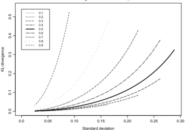
(14)

We expect the approximation(12) to get worse when the standard deviation ofX3 increases. Therefore, we have computed the Kullback–Leibler divergence as a function of Sd

(

X3

)

=

√

Var

(

X3

)

=

p

(αβ)/((α

+

β)

2

(α

+

β

+

₁

))

_{, keeping} E

(

X3

)

fixed, for a set of expected values. Varying the standard deviation, the distribution ofX3ranges from the uniform distributionU

[

0

,

1

]

to a rather peaked beta distribution. We are only considering values of

α

and

β

for which the beta distribution is either uniform or unimodal. The resulting Kullback–Leibler divergences are displayed inFig. 1. As expected, they increase with the standard deviation ofX3. Moreover, they grow with the expected value E

(

X3

)

. To better illustrate this, we have also plotted the Kullback–Leibler divergence as a function of E

(

X3

)

for a set of standard deviations, inFig. 2. We would expect the approximation to be best when the dependenceX1andX2is not too strong. As the correlation betweenX1 andX2is E

(

X3

)

, it is therefore not surprising that the Kullback–Leibler divergence(14)increases with E

(

X3

)

. Furthermore, note that(14)may be written as

DKL

(

f123

,

f

ˆ

123

)

=

E

(

−

log

(

1

−

X32

))

−

−

log 1

−

α

α

+

β

2

!!

.

Since

−

log

(

1

−

x2

)

is a convex function, Jensen’s inequality ensures not only that this difference is always non-negative, but also that it is an increasing function of the expected value E

(

X3

)

.

The Kullback–Leibler divergence enables the comparison between approximations resulting from diverse parameter sets. However, it is not a interpretable measure of the absolute quality of the approximation. Moreover, the Kullback–Leibler divergence describes a weighted average fit, down-weighting the tails due to the log-transformation. For many applications involving copulae, the main focus is actually the tails of the distribution. In such cases, the Kullback–Leibler divergence is not the most appropriate measure. Therefore, we have also computed a quantile of the sumY

=

X1

+

X2. In an application, this could typically be the Value-at-Risk of a portfolio of financial assets (with equal weights). For the true distribution, the

ξ

·

100% quantiley_ξis given by

ξ

=

P

(

Y

≤

y_ξ

)

=

Z

yξ −∞ fY

(

y

)

dy

=

Z

yξ −∞

Z

1 0 fY|3

(

y

|

x3

)

f3

(

x3

)

dx3dy

=

Z

1 0 f3

(

x3

)

Z

yξ −∞ fY|3

(

y

|

x3

)

dydx3

,

Fig. 1. Kullback–Leibler divergence between the true and the approximated distribution as a function of Sd(X3). The different curves correspond to different expected values E(X3)= {0.1,0.2,0.3,0.4,0.5,0.6,0.7,0.8,0.9}.

where the last equality follows from Fubini’s theorem. We know that

[

Y

|

X3

=

x3

] ∼

N

(

0

,

2

+

2x3

)

. Using the variable substitutionz

=

y

/

√

2

+

2x3, we obtain P

(

Y

≤

y_ξ

)

=

Z

1 0 f3

(

x3

)

Z

y_ξ √ 2+2x₃ −∞

φ(

z

)

dzdx3

=

Z

1 0 f3

(

x3

)

Φ

y_ξ

√

2

+

2x3

dx3E

Φ

y_ξ

√

2

+

2X3

,

where

φ

is the standard normal probability density. Thus, the quantile is the solution to the equation

ξ

=

E

Φ

y_ξ

√

2

+

2X3

.

(15)

In the approximated model, i.e. the simplified PCC, the distribution of the sumX1

+

X2is simply the normal distribution with mean 0 and standard deviation

√

2

+

2

ρ

. The corresponding

ξ

·

100% quantile is given by

ˆ

y_ξ

=

p

2

+

2

ρ

Φ−1

(ξ).

Fig. 3shows the relative difference between the 95% quantile from the true and from the approximated model, i.e.

(

y_ξ

− ˆ

y_ξ

)/

y_ξ, as a function of the standard deviation Sd

(

X3

)

. The various curves correspond to different expected values E

(

X3

)

. They all lie entirely under 0, which means that in this example the simplified PCC consequently overestimates the quantile, thus being conservative in a risk management sense. Moreover, the relative error increases with the standard deviation, as expected. Most importantly, the error is only one per thousand for the worst approximation (corresponding to a uniformly distributedX3). Hence, in this case, the simplified PCC is a rather good approximation.

6. Concluding remarks

In their general form, PCCs can represent most continuous multivariate distributions. However, for all practical purposes, one must resort to simplified PCCs, made of pair-copulae that depend on the conditioning variables merely through their arguments.

The simple structure, composed solely of pair-copulae, resembles Gibbs fields with bivariate interactions. Nevertheless, simplified PCCs can represent interactions between more than two variables.

Conditions for a specific decomposition of a multivariate modelnotto be of the simplified form can be expressed in terms of standard measures of dependence, more specifically Kendall’s tau, Spearman’s rho and the coefficients of tail dependence. If all conditional distributions entering the PCC belong to a location–scale family with location and scale parameters that are functions of the conditioning variables, one can also formulate conditions for the converse. Among others, one may show that elliptical distributions can be represented by simplified PCCs as long as their scale matrix is positive definite. However, further research is necessary to fully understand what the simplifying assumption signifies for the dependency.

Not all multivariate distributions can be represented by a simplified PCC. However, one can always use it as an approximation. We have shown that it may in fact be a good one, even when the simplifying assumption is far from being fulfilled. In the example we presented, the pair-copulae constituting the approximated, simplified PCC were of the same

Fig. 2. Kullback–Leibler divergence between the true and the approximated distribution as a function of E(X3). The different curves correspond to different standard deviations Sd(X3)= {0.025,0.050,0.075,0.100,0.125,0.150}.

Fig. 3. Relative difference between the true and the approximated 95% quantile ofX1+X2as a function of Sd(X3). The different curves correspond to different expected values E(X3)= {0.3,0.5,0.7,0.9}.

type as the building blocks of the exact, general PCC. This need not be the case. One should simply choose the best-fitting pair-copulae. In many cases, it is also probable that the approximation is better for some of the possible decompositions than for others. This is a matter we have not addressed in this paper, and may be a subject for future work.

Acknowledgments

This work is funded by Statistics for Innovation,

(

sfi

)

2_{. We thank Odd Kolbjørnsen for pointing out the problem that} originated in this work, and Christian Genest for the helpful discussions. We would also like to thank the participants of the Second Vine Copula Workshop in Delft, December 2008, for important discussions on the theme of vines. Finally, we thank the referees for helping us to improve the paper with their good comments and suggestions.

Appendix

A.1. Computations forExample 3.1

In order to check whether the two remaining decompositions (conditioning on X1 andX2, respectively) are of the simplified form, we must compute the copula densities

c3−i,3|i

(

F3−i|i

(

x3−i

|

xi

),

F3|i

(

x3

|

xi

)

;

xi

)

=

f3−i,3|i

(

x3−i

,

x3

)

f3−i|i

(

x3−i

|

xi

)

f3|i

(

x3

|

xi

)

,

The numerator of(16)is given by f3−i,3|i

(

x3−i

,

x3

)

=

f₁₂₃

(

x₁

,

x₂

,

x₃

)

fi

(

xi

)

=

(ν

+

x 2 i

)

ν+1 2 2ν+22

√

π

Γ

(

ν+1 2

)

p

1

−

ρ

2_xν +4 2 3 exp

(

−

1 2x3 x2 i

+

x23−i

−

2

ρ

xix3−i 1

−

ρ

2

+

ν

!)

.

Since the unconditional distribution of

(

X1

,

X2

)

is the (standard) bivariatet-distribution with correlation

ρ

and

ν

degrees of freedom, the marginal distribution ofXi

,

i

=

1

,

2

,

is a standardt-distribution with

ν

degrees of freedom. Moreover, the

conditional distribution of

[

X3−i

|

Xi

=

xi

]

,

i

=

1

,

2, is at-distribution with location

ρ

xi, scale

q

(1−ρ2_)(ν+x2 i) ν+1 and

ν

+

1 degrees of freedom. Hence, f3−i|i

(

x3−i

|

xi

)

=

Γ ν+2 2

√

π

Γ ν+1 2

q

(

1

−

ρ

2

)(ν

+

_x2 i

)

1

+

(

x3−i

−

ρ

xi

)

2

(

1

−

ρ

2

)(ν

+

_x2 i

)

−ν+22

,

i

=

1

,

2

.

Further, the second factor of the denominator of(16)is given by

f3|i

(

x3

|

xi

)

=

fi|3

(

xi

|

x3

)

f3

(

x3

)

fi

(

xi

)

=

(ν

+

x 2 i

)

ν+1 2 2ν+21Γ ν+1 2

x ν+1 2 +1 3 exp

−

ν

+

x 2 i 2x3

,

i

=

1

,

2

.

Hence,

[

X3

|

Xi

=

xi

] ∼

Gamma−1

ν+1 2

,

2 ν+x2 i

. Inserting this into(16), we obtain

c3−i,3|i

(

F3−i|i

(

x3−i

|

xi

),

F3|i

(

x3

|

xi

)

;

xi

)

=

Γ

(

ν+1 2

)

Γ

(

ν+2 2

)

1

+

(

x3−i

−

ρ

xi

)

2

(

1

−

ρ

2

)(ν

+

_x2 i

)

ν+22

s

ν

+

x2_i 2x3

·

exp

−

ν

+

x 2 i 2x3

(

x3−i

−

ρ

xi

)

2

(

1

−

ρ

2

)(ν

+

_x2 i

)

,

i

=

1

,

2

.

Finally, let u3−i|i

=

F3−i|i

(

x3−i

|

xi

)

=

tν+1





√

ν

+

1

(

x3−i

−

ρ

xi

)

2

q

(

1

−

ρ

2

)(ν

+

_x2 i

)





u3|i

=

F3|i

(

x3

|

xi

)

=

1

−

Q

ν

+

1 2

,

2x3

ν

+

x2_i

,

i

=

1

,

2

,

wheret_ν is the cdf of the standardt-distribution with

ν

degrees of freedom, andQ

(α,

x

)

=

Γ_Γ(α,_(α)x) is the regularised incomplete gamma function,Γ

(α,

x

)

being the complemented incomplete gamma function [30]. Thus,

√

ν

+

1

(

x3−i

−

ρ

xi

)

2

q

(

1

−

ρ

2

)(ν

+

_x2 i

)

=

t_ν−₊1₁

(

u3−i|i

)

ν

+

x2_i 2x3

=

Q−1

ν

+

1 2

,

1

−

u3|i

,

i

=

1

,

2

.

We obtain c3−i,3|i

(

u3−i|i

,

u3|i

;

xi

)

=

Γ ν+1 2

Γ ν+2 2

1

+

(

t_ν−₊1₁

(

u3−i|i

))

2

ν

+

1

!

ν+₂2

s

Q−1

ν

+

1 2

,

1

−

u3|i

·

exp

(

−

Q−1

ν

+

1 2

,

1

−

u3|i

(

_t−1 ν+1

(

u3−i|i

))

2

ν

+

1

)

=

c3−i,3|i

(

u3−i|i

,

u3|i

),

i

=

1

,

2

,

A.2. Computations forExample 3.4

All marginals of the multivariate Burr distribution are Burr distributions [20]. More specifically,

fi,...,i+j

(

xi

, . . . ,

xi+j

)

=

α

j

β

j

Q

j k=0

(θ

+

k

)

xβ_i+−_k1

α

P

j k=0 xβ_i+k

+

1

θ+j+1

,

xk

>

0

,

k

=

0

, . . . ,

j

.

The copula densities at the second level of the structure (corresponding to lines four to six in(8)) are given by

ci,i+2|i+1

(

Fi|i+1

(

xi

|

xi+1

),

Fi+2|i+1

(

xi+2

|

xi+1

)

;

xi+1

)

=

fi,i+2|i+1

(

xi

,

xi+2

|

xi+1

)

fi|i+1

(

xi

|

xi+1

)

fi+2|i+1

(

xi+2

|

xi+1

)

,

i

=

1

,

2

,

3

.

For the numerator, we have

fi,i+2|i+1

(

xi

,

xi+2

|

xi+1

)

=

fi,i+1,i+2

(

xi

,

xi+1

,

xi+2

)

fi+1

(

xi+1

)

=

α

2

β

2

(θ

+

₁

)(θ

+

₂

)(α

_xβ i+1

+

1

)

θ +1_xβ−1 i x β−1 i+2

(α(

xβ_i

+

xβ_i+2

)

+

α

xβ_i+1

+

1

)

θ+3

,

which is a bivariate Burr distribution in the two scaled variables Xk

(αxβ_i+1+1)θ+1,k

=

i

,

i

+

2. Further, fk|i+1

(

xk

|

xi+1

)

=

fk,i+1

(

xk

,

xi+1

)

fi+1

(

xi+1

)

=

αβ(θ

+

1

)(α

x β i+1

+

1

)

θ +1_xβ−1 k

(α

xβ_k

+

α

xβ_i+1

+

1

)

θ+2

,

k

=

i

,

i

+

2

.

Hence, ci,i+2|i+1

(

Fi|i+1

(

xi

|

xi+1

),

Fi+2|i+1

(

xi+2

|

xi+1

)

;

xi+1

)

=

θ

+

2

θ

+

1

(α

xβ_i

+

α

xβ_i+1

+

1

)

θ+2

(α

_xβ i+2

+

α

x β i+1

+

1

)

θ +2

(α

_xβ i+1

+

1

)

θ +1

(α(

xβ_i

+

xβ_i+2

)

+

α

xβ_i+1

+

1

)

θ+3

=

θ

+

2

θ

+

1

α

xβ_i

+

α

xβ_i+1

+

1

α

xβ_i+1

+

1

!

θ+2

α

xβ_i+2

+

α

xβ_i+1

+

1

α

xβ_i+1

+

1

!

θ+2

·

α

x β i

+

α

x β i+1

+

1

α

xβ_i+1

+

1

+

α

x β i+2

+

α

x β i+1

+

1

α

xβ_i+1

+

1

−

1

!

−(θ+3)

.

Letting uk|i+1

=

Fk|i+1

(

xk

|

xi+1

)

=

Z

xk 0 fk|i+1

(

y

|

xi+1

)

dy

=

1

−

α

x β i+1

+

1

α

xβ_k

+

α

xβ_i+1

+

1

!

θ+1

,

k

=

i

,

i

+

j

,

such that

α

xβ_k

+

α

xβ_i+1

+

1

α

xβ_i+1

+

1

=

(

1

−

uk|i+1

)

− 1 θ+1

,

_k

=

_i

,

_i

+

₂

,

we obtain ci,i+2|i+1

(

ui|i+1

,

ui+2|i+1

;

xi+1

)

=

θ

+

2

θ

+

1

(

1

−

ui|i+1

)

−θ_θ+₊2₁

(

1

−

ui+2|i+1

)

− θ+2 θ+1

·

((

1

−

ui|i+1

)

−_θ+1₁

(

1

−

ui+2|i+1

)

−_θ+1₁

−

1

)

−(θ+3)

=

ci,i+2|i+1

(

ui|i+1

,

ui+2|i+1

),

i

=

1

,

2

,

3

.

Correspondingly, the third level copula densities (lines seven and eight of(8)) are given by ci,i+3|i+1,i+2

(

Fi|i+1,i+2

(

xi

|

xi+1

,

xi+2

),

Fi+2|i+1,i+2

(

xi+3

|

xi+1

,

xi+2

)

;

xi+1

,

xi+2

)

=

fi,i+3|i+1,i+2

(

xi

,

xi+3

|

xi+1

,

xi+2

)

fi|i+1,i+3

(

xi

|

xi+1

,

xi+2

)

fi+3|i+1,i+2

(

xi+3

|

xi+1

,

xi+2

)

,

i

=

1

,

2

,

with fi,i+3|i+1,i+2

(

xi

,

xi+3

|

xi+1

,

xi+2

)

=

α

2

β

2

(θ

+

₂

)(θ

+

₃

)(α

_xβ i+1

+

α

x β i+2

+

1

)

θ +2_xβ−1 i x β−1 i+3

(α(

xβ_i

+

xβ_i+3

)

+

α

xβ_i+1

+

α

xβ_i+2

+

1

)

θ+4

,

and fk|i+1,i+2

(

xk

|

xi+1

,

xi+2

)

=

αβ(θ

+

2

)(α

xβ_i+1

+

α

x_iβ₊₂

+

1

)

θ+2_xβ−1 k

(α

xβ_k

+

α

xβ_i+1

+

α

xβ_i+2

+

1

)

θ+3

,

k

=

i

,

i

+

3

.

We obtain ci,i+3|i+1,i+2

(

Fi|i+1,i+2

(

xi

|

xi+1

,

xi+2

),

Fi+3|i+1,i+2

(

xi+3

|

xi+1

,

xi+2

)

;

xi+1

,

xi+2

)

=

θ

+

3

θ

+

2

α

xβ_i

+

α

xβ_i+1

+

α

xβ_i+2

+

1

α

xβ_i+1

+

1

!

θ+3

α

xβ_i+3

+

α

xβ_i+1

+

α

xβ_i+2

+

1

α

xβ_i+1

+

α

xβ_i+2

+

1

!

θ+3

·

α

x β i

+

α

x β i+1

+

α

x β i+2

+

1

α

xβ_i+1

+

α

xβ_i+2

+

1

+

α

x β i+3

+

α

x β i+1

+

α

x β i+2

+

1

α

xβ_i+1

+

α

xβ_i+2

+

1

−

1

!

−(θ+4)

.

Finally, we substitute with

uk|i+1,i+2

=

Fk|i+1,i+2

(

xk

|

xi+1

,

xi+2

)

=

1

−

α

x β i+1

+

α

x β i+2

+

1

α

xβ_k

+

α

xβ_i+1

+

α

xβ_i+2

+

1

!

θ+2

,

k

=

i

,

i

+

3

,

and obtain ci,i+3|i+1,i+2

(

ui|i+1,i+2

,

ui+3|i+1,i+2

;

xi+1

,

xi+2

)

=

θ

+

3

θ

+

2

(

1

−

ui|i+1,i+2

)

−θ_θ+₊3₂

(

1

−

ui+3|i+1,i+2

)

− θ+3 θ+2

·

((

1

−

ui|i+1,i+2

)

− 1 θ+2

(

₁

−

ui+3|i+1,i+2

)

− 1 θ+2

−

1

)

−(θ+4)

=

ci,i+3|i+1,i+2

(

ui|i+1,i+2

,

ui+3|i+1,i+2

)

i

=

1

,

2

.

Corresponding computations for the top level copula densityc15|234results in

c15|234

(

u1|234

,

u5|234

;

x2

,

x3

,

x4

)

=

θ

+

4

θ

+

3

(

1

−

u1|234

)

−θ_θ+₊4₃ <