Sampling Strategies for Error Rate Estimation and Quality Control

(1)

Project Number: JPA0703

Sampling Strategies for Error Rate

Estimation and Quality Control

A Major Qualifying Project Report Submitted to the faculty

of the

Worcester Polytechnic Institute in partial fulfillment of the requirements for

the Degree of Bachelor of Science in Actuarial Mathematics

by

__________________________ ____________________________ Nicholas Facchiano Ashley Kingman

__________________________ ____________________________ Amanda Olore David Zuniga

Date: April 2008 Approved by:

____________________________ _____________________________ Jon Abraham, Project Advisor Jayson Wilbur, Project Advisor

(2)

1

Table of Figures

Figure 1.1: Depiction of data range used in a two-sided confidence interval Figure 1.2: Depiction of data range used in a one-sided confidence interval Figure 1.3: Screenshot of Sampling Optimization Worksheet Sheet 1

Figure 1.4: Screenshot of Sampling Optimization Worksheet Sheet 2 Figure 1.3: Sample Size versus Total Cost with C_s=$5and C_t= $1000

Figure 1.4: Three-Dimensional Projection of Resultant Sample Size as a function of varying per sample and per trait costs

Figure 2.1: Histogram of Company Shortfall Amounts Figure 2.2: Bootstrapping Steps

Figure 2.3: Bootstrapping Program Input Worksheet Figure 2.4: Input Worksheet – John Hancock Data

(5)

4

Table of Tables

Table 1.1: Binomial sample sizes with corresponding margins of error Table 2.1: Example of Bootstrapping Program Output

Table 2.2: Bootstrap Program Results Table 3.1: Defective vs. Non-Defective Table 3.2: MS Tool Descriptions

Table 4.1: Worker Differences

Table 4.2: Level of Confidence Variation Table 4.3: Population Variation

(6)

5

Abstract

John Hancock must utilize processes to monitor departmental performance. Our group was presented with several problems whose solutions will benefit the company’s quality assurance capabilities. This MQP analyzes the optimization of a sampling function for a book of insurance policies, the Bootstrapping method for the estimation of policy shortfall confidence intervals, and a sampling procedure to aid the company in customer satisfaction screening.

(7)

6

Executive Summary

John Hancock is a leader in the insurance and financial service industry. The company must utilize quality control procedures to monitor departmental performance. The objective of this project was to develop sampling strategies for the estimation of error rates and means in an effort to improve current quality control processes.

John Hancock requested the development of a sampling methodology to estimate the proportion of defects within a book of life insurance policies. Defective policies carry a liability which must be paid to the policy holder. Our group was able to optimize a preexisting sampling function by introducing constraints for liability cost and sampling cost. This new function will allow John Hancock to take a properly sized sample which minimizes the total project cost for the given parameters.

The second initiative involves the estimation of a confidence interval for mean shortfall amount. Statisticians often use a method known as Bootstrapping to create larger data sets by taking random samples from initially small samples. The key assumption in this process is that the sample data is representative of the entire data set. With the newly created data set, we were able to estimate an interval for mean shortfall amount given a desired confidence level.

Lastly, John Hancock consults with a call center to monitor customer satisfaction. Each call center employee has his/her work screened on a monthly basis; currently, each employee is sampled five times per month. However, this sample size has no statistical significance. The goal is to create a tool which will provide John Hancock with a properly sized sample of work items to screen for each employee. The resultant sample size is a function of historical employee performance and desired confidence.

(8)

(9)

8

Introduction

The main focus of this project is statistical analysis. Overall, statistics is a very broad subject. Many topics were explored in order to propose statistically sound recommendations regarding John Hancock’s quality control efforts. Types of distributions, estimators of population parameters, and confidence levels and intervals were only some of the topics that were researched in order to achieve our goal.

The John Hancock Company, established in 1862, provides consumers with a variety of financial services. It is one of the top life insurance companies in the nation in sales. The company strives to maintain this position through the development of new financial products and quality assurance. These approaches to maintaining market share are incorporated into every area of the company, including sales, marketing, finance, and customer service.

For this Major Qualifying Project, John Hancock proposed a question involving current quality assurance (QA) efforts. Although QA efforts exist within the company, there is no statistical significance regarding the amount sampled. The goal of this project was to develop statistically significant sampling strategies for four different scenarios involving error rate and mean estimation. A major problem surrounding the scenarios is the lack of statistical understanding within the department. In order to ensure employees are providing the best support possible, the department needs to be able to take representative and random samples of data and calculate estimates for population error rates and means while being as cost effective as possible.

To obtain statistically significant results, the group researched estimators, distributions, confidence levels and intervals, margin of error, finite and infinite populations, and resampling methods. The four scenarios were addressed independently of each other in order to obtain sampling methods tailored to the particular problem. Programs were created in Excel in order to facilitate calculations. The rest of this report details the background research performed for each problem, their methodologies, the data and analysis, and conclusions. Instructions to the Excel spreadsheets are also included.

(10)

9

I. Sampling Optimization

1. Background

The John Hancock Life Insurance Company proposed that a sampling strategy be developed for a group of life insurance policy holders in an effort to estimate the frequency of policies with a particular trait; the hope is that we can establish an accurate error rate without reviewing every policy. Assuming there are limitations on sampling capability, such as a maximum sample size a

department can undertake, we must factor in cost constraints to optimize our sample size for total procedure cost. It is important to understand several key statistical concepts prior to analyzing the function derivation.

2. Methodology

Confidence

Confidence intervals are used to assess the precision of an estimate; given that a population proportion estimate is computed, it is necessary to construct an interval about the estimate to account for sampling error. When

constructing a confidence interval for an error rate, we are presented with two options. The two-sided confidence interval allows us to be 100(1-α)% confident that the true error rate lies within bounds that are equidistant from the estimated error rate. The one-sided confidence interval allows us to be 100(1-α)%

confident that the true error rate lies below an upper bound. Using higher levels of confidence yields larger intervals, because widening an interval increases the probability of containing the true error rate (Thompson, 2002).

(11)

10

Two-Sided Confidence

Depiction of data range used in a two-sided confidence interval (Figure 1.1)

One-Sided Confidence

(12)

11

Sample Proportion

The sample proportion pˆ is the percentage of the sample taken that reflects a given trait or quality. If we were to sample ten policies, with two being defective, our sample proportion pˆ would be equal to 2/10, or 20%.

Margin of Error

The margin of error summarizes sampling error and quantifies the uncertainty of an estimate. As the sample size increases, the margin of error decreases; this is due to the fact that larger samples decrease uncertainty about population parameters. Figure 1C displays sample sizes and

corresponding margins of error for a binomial distribution with population error rate of 50%. For example, with a sample size of 96, the margin of error is 10%.

(

)

(

)

96 5 . 0 1 5 . 0 10 . 0 2 025 . − = Z Sample

Size Margin of Error

96 10%

384 5%

600 4%

1067 3%

2401 2%

Binomial sample sizes with corresponding margins of error (Table 1.1)

Initial Sampling Function

The Central Limit Theorem (CLT) states that the sums or means of random samples of independent and identically distributed (iid) random variables with finite variance will be approximately normally distributed. If N (population size), n (sample size) and N-n are sufficiently large, then the sampling distribution of

n S N n y − − 1

µ

is approximately normal with mean 0 and variance 1 (S refers to the

(13)

12

the population mean is 

     − + − − n S N n Z y n S N n Z y _α₂ 1 , _α₂ 1 . If we view the margin of error as n S N n

Z_α₂ 1− we can obtain absolute precision in our sample

size. Solving for n we get

n S N n Z e= _α₂ 1− ; we must hold 2 e fixed in N S Z e S Z n ₂ ₂ 2 2 2 2 2 α α +

= or else the equation reduces ton=n. When sampling from a

population as large as the block of life insurance policies as discussed in the background, the denominator piece with Ntends to zero and can be removed,

leaving us with ₂ 2 2 2 e S Z n α

= (Lohr, 1999). Since we are constructing a one-sided

confidence interval, we will use ₂ 2 2 e S Z n= α in place of ₂ 2 2 2 e S Z n= α . n S N n y − − 1

µ

(1)       − + − − n S N n Z y n S N n Z y α2 1 , α2 1 (2) n S N n Zα2 1− (3) n S N n Z e= α2 1− (4) N S Z e S Z n ₂ ₂ 2 2 2 2 2 α α + = (5)

(14)

13 2 2 2 2 e S Z n= α (6) 2 2 2 e S Z n= α (7)

After using a confidence level of 99%, a sample proportion of 1%, a margin of error of 0.1%, and a population size of 5,000,000 our resultant sample size is 53,578 (See Equation 8).

(

)

(

)

(

0.001

)

53,578 01 . 0 1 01 . 0 326 . 2 2 2 2 2 2 2 = − ⇒ = e S Z n α (8)

While this may be the optimal sample size for the given parameters, there are constraints lacking from the function that must be accounted for. These factors stem from issues based upon the John Hancock Governance & Product Support Department’s ability to cover the financial aspect of such a sampling project. Assuming that there are liabilities inherent within each population error and a cost necessary to provide a particular sample size, these two parameters will provide the information necessary to establish the point at which a trade-off arises between the cost associated with sampling and the liability/trait cost. The goal is to minimize the total cost of this sampling operation (Lohr, 1999).

3. Analysis & Discussion

Cost Function Derivation

As noted previously, a formula which accounts for procedure costs will allow us to quantify the financial impact of sampling from the block of insurance policies. The per trait cost is the liability cost associated with each error from the insured policies; it is denoted as Ct. The per sample cost is the cost associated

with taking one sample – i.e. reviewing one insurance policy to determine its status as being defective; it is denoted as Cs. When formulating the two pieces

(15)

14

to this cost function, one piece is attributed to the total sampling cost and one piece for the total trait cost. The total sampling cost is the product of the per sample cost with n, the sample size. The total trait cost is the product of the per trait cost, population size, and the upper bound to the population error rate; effectively, this is the product of the number of defective policies with the per trait cost. t s N p e C nC n f( ) (ˆ ) Cost Trait Cost Sampling Cost Total + + = + = (9)

Optimization Function Derivation

If we allow n, the sample size, to be our variable, then we can optimize the cost function for all inputs C_s and C_t. This will allow the John Hancock Governance and Product Support Department to design a sampling strategy that will make the best use of its sampling capabilities. The total sampling cost and total trait cost behave in a fashion similar to that of the relationship

between sample size and margin of error. As one takes larger samples, the margin of error and upper bound to the population error rate are reduced. Likewise, with a larger sample comes a larger total sampling cost. However, the total trait cost is reduced since the upper bound to the population error rate is lower. The ideal situation occurs when the optimal sample size is reached; this sample size minimizes the cost of the entire procedure for the given parameters – it balances the negative impact of increased sampling cost with the benefit of decreased trait cost. The following formulae illustrate the mathematics involved in arriving at the optimization function. Differentiate Equation 9 with respect to n and arrive at Equation 10. After rearranging terms and solving for n, we are left with an optimization function for sample size; this result is displayed as Equation 11.         ₋ − + = 2 3 2 ' 2 1 ) ˆ 1 ( ˆ ) ( n p p Z NC C n

(16)

15

(

)

2/3 2 2 ) ˆ 1 ( ˆ         ₋ = s t C p p Z NC

n α (11: Final result for optimized sample size)

MS Excel Tool Development

In order to further assist John Hancock in their sampling endeavors, a worksheet was created in Microsoft Excel to compute optimal sample sizes and cost projections for given parameters and cost constraints. The user inputs in this excel program are Population, Confidence Level, Sample Proportion, Per

Sample Cost, Per Trait Cost, and Sample Errors; the Sample Errors input is the number of errors found within the optimal sample. For the given parameters and cost constraints, the sheet computes Sample Size, Sampling Cost, Trait Cost, and Total Cost.

(17)

16

Screenshot of Sampling Optimization Worksheet Sheet 2 (Figure 1.4)

4. Results and Conclusions

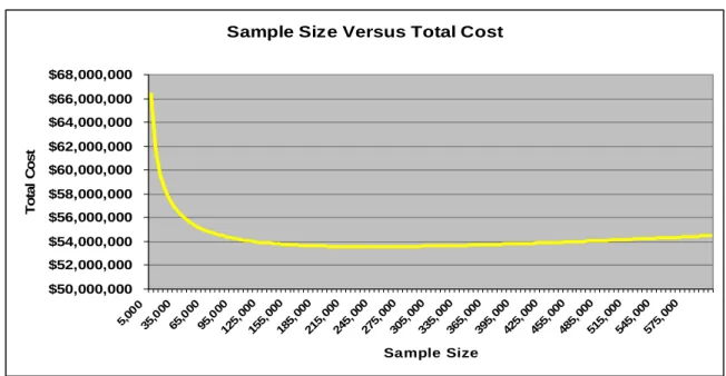
As a result of the optimization function, the John Hancock Governance and Product Support Department can assess the available resources to sample and weigh the financial implications of a specific sampling strategy with other pressing departmental issues. The functions were built into a Microsoft Excel worksheet; this tool Excel is essential in giving John Hancock the ability to find optimal sample sizes and total cost projections for various sampling operations. The following graphic illustrates the behavior of the total cost with respect to sample size for a per sample cost of $5 and a per trait cost of $1,000. The

optimization function attains its minimum at the optimal sample size of 237,488 – the cost associated with this sample size is $53,562,318 (As seen in Figure 1.5).

(18)

17 Sample Size Versus Total Cost

$50,000,000 $52,000,000 $54,000,000 $56,000,000 $58,000,000 $60,000,000 $62,000,000 $64,000,000 $66,000,000 $68,000,000 5,0 00 35, 000 65, 000 95, 000 125 ,000 155 ,000 185 ,000 215 ,000 245 ,000 275 ,000 305 ,000 335 ,000 365 ,000 395 ,000 425 ,000 455 ,000 485 ,000 515 ,000 545 ,000 575 ,000 Sample Size T o ta l C o s t

Sample Size versus Total Cost with C_s=$5and C_t= $1000 (Figure 1.5)

Figure 1.6 depicts the behavior of the resultant optimal sample size for varying Cs and Ct. For fixed per trait cost, we see that it is logical to take larger

samples as per sample cost tends to zero. For fixed per sample cost, we see that it is logical to take larger samples as per trait cost grows.

(19)

18

II. Universal Life Policies

1. Background

As a provider of financial services, John Hancock is faced with a significant problem when there are company shortfalls on life insurance

products. The company would benefit greatly by knowing the exact number and amount of these shortfalls; however, calculating values for all contracts would be unrealistic given that sampling a single contract takes a significant amount of time and it is unknown if a contract even contains a shortfall. It was determined that knowing the mean amount of a shortfall (given there was one) with a certain level of confidence would provide a sufficient amount of

information. Representatives from John Hancock provided our group with data on 50 Universal Life Contracts, 37 of which contained company shortfalls. A histogram of these shortfall amounts is shown in Figure 2.1.

Histogram of Company Shortfall Amounts (Figure 2.1)

Using this data, John Hancock wanted to obtain an estimate for the mean and a 95% confidence interval for this estimate. The company also sought a

(20)

19

T Distribution

The group’s first inclination concerning this data was to use the standard t-interval, as shown below:

(12)

Where is the t-statistic with confidence and the other statistics are as follows:

(13)

(14)

(15)

However, due to the presence of an outlier in the original data (as seen in Figure 2.1), it was decided that a more appropriate alternative existed(PETRUCCELLI, NANDRAM, & MINGHUI, 1999).

Bootstrapping

The Bootstrap Method is a resampling technique which “avoids unverified parametric assumptions by relying solely on the original sample” (Chernick, 1999). We must assume, however, that the original sample is both

representative of the population and randomly chosen. The method consists of six main steps:

1. Obtain an original sample of size n.

2. Assign probability 1/n to each data point in the original sample. This ensures that each data point has the same probability of being chosen.

3. Sample with replacement from the original sample to generate a bootstrap sample of size m.

(21)

20

4. Compute the mean of the bootstrap sample.

5. Repeat steps 3 and 4 B times, creating B bootstrap samples of size m and their means.

6. Calculate the mean of the bootstrap sample means to obtain an estimate for the population mean.

A diagram of these steps can be seen in Figure 2.2 below:

Bootstrapping Steps (Figure 2.2)

Once B bootstrap sample means have been computed, a confidence interval for the mean of the bootstrap sample means can be determined using the percentile method. The percentile method involves ordering the bootstrap sample means and determining an interval which contains 100(1-α)% of the values, where 100(1-α) is the desired confidence level. The confidence interval width is then found by subtracting the lower limit of the confidence interval from its upper limit. In order to obtain a confidence interval for the mean within the desired width, the size of the bootstrap sample, m, should be increased until the desired width is reached. This is because the bootstrap sample size, m, has a larger influence on the confidence interval width than B, the number of bootstrap samples.

(22)

21

2. Methodology

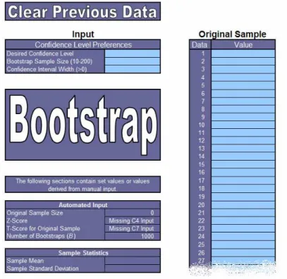
In order to decrease the time spent calculating the mean of B bootstrap samples as well as its corresponding confidence interval, a bootstrapping program was created. To run the bootstrapping program, four inputs are necessary, including:

1. Desired Confidence Level 2. Bootstrap Sample Size, m

3. Desired Confidence Interval Width 4. Original Sample

Figure 2.3 contains a screenshot of the bootstrapping program input worksheet. Specific instructions regarding use of the program can be found in Appendix 1.

Bootstrapping Program Input Worksheet (Figure 2.3)

After inputting this information, the program is run by clicking the

(23)

22

computes their mean, and then outputs an estimate for the mean equal to the mean of the bootstrap sample means, a confidence interval for the estimate, and the width of the given confidence interval. The confidence interval is computed using the percentile method. After the bootstrap sample means are sorted increasingly, the lower limit equals the bootstrap sample mean which falls after 100(α/2)% of the values and the upper limit is the bootstrap sample mean which falls before the largest 100(α/2)% of the values. It is important to note that this method while this method produces an (approximately?) equal-tailed

confidence interval, it will almost never produce a confidence interval with limits that are approximately an equal distance from the mean unless the distribution of the bootstrap sample means approaches the normal (or symmetric)

distribution. When the width of the confidence interval is less than the user’s desired width, the line will be highlighted in yellow.

Upon completion of these calculations, a new row is inserted into the table on the ‘Output’ worksheet, the calculated values are filled in, and the table is sorted in descending order first according to sample size m. then according to the confidence interval width. For comparison, the mean and confidence interval found using the t distribution are also included. The code used in Excel to perform the bootstrap is shown in Appendix 2.

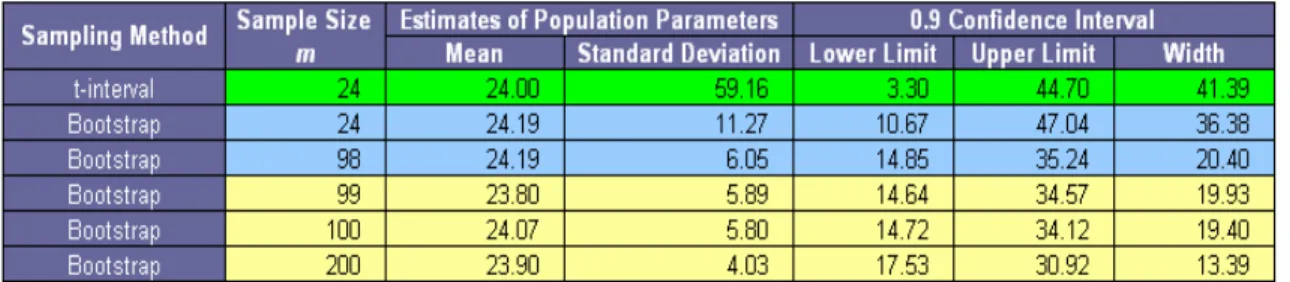
To provide an example of the program’s output, bootstraps were run on a sample consisting of all the integers from 1-23 and 300, to make an original sample with size n = 24. The specified confidence level and width were set at 90% and 20, respectively.

(24)

23

Example of Bootstrapping Program Output (Table 2.1)

Table 2.1 contains the program output according to the specified conditions. The smallest sample size which should be taken in order to meet these

conditions is shown to be 99. This is because 99 is the smallest integer which provides a confidence interval width smaller than 20. The impact of the Bootstrapping method is evident; when using the t-interval, the confidence interval width is 41.39 but this number decreases to 19.93 when the

(25)

24

3. Analysis and Discussion

In the case of the shortfall data provided by John Hancock, the specified conditions and original shortfall data were entered into the bootstrapping

program. These included a confidence level of 95%, a desired confidence interval width of $2000, and the 37 shortfall amounts. A screenshot of this input is shown in Figure 2.4.

Input Worksheet – John Hancock Data (Figure 2.4)

The program was run according to the instructions provided in Appendix 1. Its results can be found in Table 2.2.

(26)

25

In order to determine a solution, a series of bootstraps were run. For the first bootstrap sample, m was set equal to 37. Due to its confidence interval width ($3242.86) being larger than desired ($2000), the size of the bootstrap sample, m, needed to be increased. First, however, m was set equal to 200 in order to see if the program was capable of calculating a confidence interval according to specifications. This bootstrap was within the desired size, having a width of only $1399.99. From this point, educated guesses were made as to the value of m which would bring the confidence interval width below $2000. As shown in Table 2.2, when the bootstrap sample size increased from 106 to 107, the confidence interval width dropped below $2000 (from $2049.63 to $1946.12).

Bootstrap Program Results (Table 2.2)

(Confidence Level = 95%, Desired Confidence Interval Width = $2000)

This table shows that according to the original data set and specifications provided by John Hancock, the company needs to sample until 107 shortfall amounts are obtained. Figure 2.5 below illustrates the distribution of the

bootstrap sample means when m = 107 and indicates the lower and upper limits for the confidence interval.

(27)

26

Histogram of Bootstrap Sample Means with Confidence Interval Limits (Figure 2.5)

If the company is willing to sample more than 107 shortfalls, a confidence level of 99% meeting the same criteria can be met if 184 shortfalls are sampled.

Alternatively, if John Hancock is not willing to sample 107 shortfalls, a confidence level of 90% can be reached if 73 shortfalls are sampled. With the current

sample size of 37, the bootstrap method produced a mean of $2,411.44 and a confidence interval (95% confidence level) with a width of $3,242.86.

4. Results and Conclusions

The bootstrapping method proves especially useful when data is skewed or contains a heavy tail. It can also be used to alert the user to variability in the data. However, it is important to only use the Bootstrapping Method in

appropriate situations. This method can be used in a number of situations, so John Hancock must be wary of using the Excel program in cases where more appropriate alternatives exist.

It was decided the Bootstrapping Method would be fitting for the shortfall data presented to the group due to the presence of an outlier. After

developing the bootstrapping program, it was determined that in order to obtain a confidence interval for the estimate of the mean with a confidence level of 95% and a width of less than $2000, a sample of at least 107 shortfalls needed to be taken. Note that this does not refer to the total number of

(28)

27

policies sampled, but the number of policies sampled which contain a company shortfall.

The Excel program which the group created will allow John Hancock to use the Bootstrapping Method and avoid parametric assumptions when working with a small original data set. It will be useful when the company is dealing with similar situations in the future.

(29)

28

III. NWI Tracking

1. Background

Large companies like John Hancock perform many quality assurance tests in order to monitor how well their customer service employees and

processes are performing. The goal of quality assurance testing is to control errors or problems and to increase efficiency within a certain group or process.

Quality Assurance

Companies are very aware of the importance of delivering products or services as economically as possible due to fast-developing technology,

increasing operational complexity, and high competition. These circumstances put a premium on effective quality assurance concepts that are capable of helping a company achieve these objectives. All kinds of organizations find quality assurance (QA) vital to their success. However, each organization’s quality assurance plan will be different since each organization is unique with its own unique set of customer needs.

Quality assurance consists of “all the planned and systematic actions that provide confidence to an organization” that its product or service will offer satisfaction to its customers. A relevant term associated with quality assurance for this project is testing, which refers to “an evaluation of the performance of a [service].” (Lloyd, 1980) This occurs with the sponsor’s customer service division, which handles inquiries from its customers on a daily basis.

The particular service which concerns this project are the thousands of phone calls handled by the customer service staff, a portion of which are also QA tested to ensure that the customers’ issues are being dealt with

appropriately. Many companies, like John Hancock in this case, outsource QA testing to specialty consultants who excel in this area of work. (Lloyd, 1980)

(30)

29

Data

The NWI (New Work Item) Tracking data that was provided to the group was a set of QA tests done on customer service department. The tests involved the scoring of employee handling of customer phone calls received by

customer service representatives. The data relate to calls received between January and September of 2007.

Current policy is for new customer service representatives to have a high percentage of their customer phone calls screened and scored/graded until they have worked a certain number of months with the company. After this period, each experienced customer service representative has 4-5 calls randomly chosen each month to be scored by the 2 testers. The scoring is based on 3 categories: Accuracy (40pts), Necessity (40pts), and Comments (20pts). For each category, the tester marks down Y or N which totals an overall score for the call.

The goal of this: Why are the QA testers sampling 4-5 calls per month for each experienced representative? The company would like to know which sample size would be the most efficient estimate of the true error rate in the population of calls.

Hypergeometric Distribution

The hypergeometric distribution is a discrete probability distribution which arises in relation to random sampling (without replacement) from a finite population. This describes the distribution of scored customer service calls within the sample taken, as the QA testers select random calls to score thus removing these calls from the sampling population (without replacement).

The following table is a contingency table which helps illustrate a typical example:

(31)

30

Drawn Not Drawn Total

Defective K m-k m

Non-Defective n-k (N-m)-(n-k) N-m

Total N N-n N

Defective vs. Non-Defective (Table 3.1)

Consider a box containing N widgets, of which m are defective. Now draw a random sample of n balls such that every sample of size n has the same chance of being selected. The random variable of interest is the number (k) of defective widgets in the sample. The probability of seeing k defective widgets in a sample of n widgets is given by the probability density function of the Hypergeometric distribution:

(16)

In this case “defective” would be calls not scored 100 by the QA testers. The drawn number (n) includes the total number of scored calls for each

customer service employee since January 2007 (where the data begins). The total population of calls (N) includes all of the calls handled by each employee, even though not all have been sampled for scoring. The defective calls are the number of calls (k) that have not been scored 100 by the QA testers in the sample taken for each employee (Goetz, 1978).

Binomial Distribution

Consider a set number of n mutually independent Bernoulli trials. A Bernoulli trial can be defined as a random experiment in which only two

outcomes exist, either “failure” (or 0) or “success” (or 1). Assume that all of these trials have the same success proportion p. The Binomial Distribution is a discrete distribution for the total number of successes (k) in the n trials. The probability of

(32)

31

seeing k successes in n trials with probability of success p is given by the probability mass function for the Binomial distribution.

(17)

In this instance, an error is considered to be a success. The distribution of total errors in the population is modeled by a binomial distribution, as it is

assumed each customer service call is independent, and the probability p of seeing an error (score not equal to 100) is assumed to be the proportion of errors found in the sampled calls (k/n) (Goetz, 1978).

2. Methodology

First, an error needed to be clearly defined, since each QA test could have a range of different scores due to the multiple scoring categories. The group decided it was logical to classify an error as any tested call that was NOT scored as 100. Secondly, since many new employees had large amounts of calls tested each month, only experienced employee tested calls were used. This was done to eliminate any skewed data due to new employees having higher error rates because of a lack of experience.

The distribution was observed and checked to see if the error rate was affected by any factors such as work experience or the QA testers. Appendix 4 presents a description of each tab created to analyze the data (NWI Tracking sheet 11-26).

Not much information is known regarding the experience of the testers nor is it known how they determine an error in each category. The ultimate goal is to find the best number of tests to take from each individual per month in order to get the best estimate of the true error rate. The most likely result is a estimated sample size.

(33)

32

The team looked to build a tool in Microsoft Excel that would be able to produce such a sample size for each individual customer service employee. The distribution of the errors (not a score of 100) is that of a Hypergeometric distribution, and we were looking for the probability that there exist m total errors in the entire population (N) of calls by the employee since January given there are k number of errors in the sampled number of calls for each employee since January ( “P( m | k )” ). Using the definition of conditional probability:

(18)

The definition is used twice to obtain the numerator of the second part of the equation, while Bayes Rule can be used to get its denominator.

(Handbook of Applicable Mathematics: Volume II – Probability p35, this will be properly cited eventually)

Several Microsoft excel functions are capable of calculating these probabilities given a few inputs (N, n, k) for each employee. The probabilities are calculated for the distribution of total number of errors (m) possible given these input values. The following is a description of how the tool works:

First, the population of total calls (N) handled by the employee is

entered, along with the total number of sampled calls (n) since January and the number of those calls found to have an error (k). The table displays the different probabilities in the equation above for each m* possible (Column F).

NWI Tracking MS Tool Descriptions

Column Description

G Displays the P(m=m*) which is described by the Binomial distribution with N trials and p = k/n. The function

BINOMDIST calculates the probability of seeing m* errors in N independent trials, each with probability p.

(34)

33

H Finds the P( k|m ) which is described by the

Hypergeometric distribution. The function HYPGEOMDIST

calculates the probability that there are k (input) errors found in the sample of n (input) given that there are actually m* errors in the call population size N (input). I Shows the P( m=m*|k ) which is equal to the product of

probabilities as described above. For each m*, column I calculates the quotient of the product of P( m=m* ) and P( k|m=m* ) (column G * column H), and the sum of all products of P( m=m* ) and P( k|m=m* ).

J Produces the CDF of P( m=m*|k ) by simply summing column I from

m*=0 to m*, which is also the display of the level of confidence that

P( m=m*|k ) ranges from the lowest m* possible (k) to m*.

MS Tool Descriptions (Table 3.2)

3. Analysis and Discussion

Now that the distribution of errors has been obtained, the derivation of a sample size can be looked at. Since the distribution is best described as

hypergeometric, the upper bound on a hypergeometric confidence interval can be used to find the new sample size. The resulting derived equation for the new sample size for a hypergeometric distribution is:

(19)

The finite population correction factor is represented in the first quantity in the numerator of the fraction, which takes into account the total population of calls N and the initial sample size n₁ . The margin of error e is found in the denominator, along with the test statistic of the normal distribution given a confidence level α. The remaining element is a good estimate of the true error rate.

(35)

34

In order to obtain this estimate, the expected number of errors was found. The MS tool calculates E(X) (cell C8) by summing the products of Column F (m # of errors in the population) and Column I (the probability of m errors given k

errors in the sample). This expected value is then divided by the total population size (cell C4), to produce the Estimated Error Rate in cell C10.

Now that a good estimator of the error rate has been obtained, the sample size function can be used. The user of the tool must input a desired confidence level into cell C11, as well as a desired margin of error into cell C13. The margin of error is putting a bound on true error rate of the population given the desired confidence, sample size, and estimated error rate. The smaller margin of error desired, the more sample size will be needed to satisfy the

desired confidence. The optimal hypergeometric sample size given the desired inputs is displayed in cell C15.

4. Results & Conclusions

With this MS tool, John Hancock can more accurately sample each

individual customer service representative according to their past scoring results, rather than arbitrarily sampling each employee 5 times per month. The functions built in this MS tool allows John Hancock to provide a desired level of

confidence and margin of error in the sampling process, which will help provide more acute sampling of the more error-prone employees. John Hancock will be able to quickly identify which employees need to improve their ability to handle phone calls from customers.

Since each employee is different, there are some scenarios where the employee has very few errors out of a large number of sampled calls. In these cases, the hypergeometric sample size is shown to be some negative number. This is suggesting that there is no reason to sample from this employee since they have such a low estimated error rate. However, it would be beneficial to sample some number from these employees, just so there is some historical data for

(36)

35

each month moving forward. The number can be some arbitrary low number, preferably between 1 and 5.

(37)

36

IV. Variable Surrender

1. Background

Definition of the Problem:

Currently, John Hancock is performing quality control at one hundred percent for all variable loans. This is to insure that all of the loans are processed within the day that they are received or on their effective date. This section looks in depth into variable life policies. John Hancock defines Variable Life policies as a “permanent life insurance, which allows you to invest a portion of your premium in stocks, bonds, or money market subaccounts in order to build your policy's cash value.” (John Hancock, 2008)Because these policies are considered

investment products, they are regulated by the Securities and Exchange Commission (SEC). By law, the SEC must oversee all transactions made in

investment products. The main goal of this portion of the project was to find out if John Hancock could reduce their sampling rate below one hundred percent for their Variable Life policies.

Statistical Properties

The variable surrender data is taken on a monthly basis. Any calls

regarding a Variable loan processed in the month are recorded in an Excel file. Because of this, there is not a lot of data to work with month by month.

Typically, John Hancock only sees between 1200 to 1500 variable surrenders a month. Since we are trying to calculate a sample size, there is a basic equation that can be used:

2 2 2 e S Z n= α (7)

(38)

37

The variables are: -the sample size, - the Z-score for the normal distribution, - the assumed probability that an error will occur, and - the margin of error. Unfortunately, the above equation does not work for a finite population, which is what we are looking at for this distribution of data. However, we can create a new equation from the original by utilizing what statisticians call the population correction proportion. This helps to normalize the data and changes the above equation to:

N S Z e S Z n ₂ ₂ 2 2 2 2 2 α α + = (5)

The variables for this equation are all the same except for which is the total population of the data. The team will be utilizing equation (5) for this segment of the project (Lohr, 1999).

2. Methodology

Errors

Variable Loan surrender data looks at two different errors: effective date errors and transfer errors. Effective date errors occur when a loan is not looked at (or QC’ed) on the date received. Because of SEC standards, these loans need to be QC’ed by 4 PM every day. This error occurs approximately five percent of the time in any given month. Transfer errors happen when a customer is allowed to transfer funds from the account more than twice a month. This is not supposed to happen, and John Hancock needs a zero

percent error rate for this type of error. When either of these errors takes place, it is recorded in the variable surrender data. However, for this project, the main objective was to look into the effective date errors.

(39)

38

Process

To organize the data, many indicators were made in the original datasheet pointing out various changes in the data. Using Microsoft Excel, formulas were created to pick out the data necessary for analysis. For example, in the original data, there was a column for “Effective Date Errors.” However, it indicated how long it took to process a particular surrender, but not simply indicate if there was an error. A formula was created in another column in the workbook that stated, “If the effective date error column was equal to zero, place a zero in the cell; if not, place a one in the cell.” This created a way to count all of the effective date errors by just taking the summation of the column of cells. These columns contain what are called indicator functions. Many other indicator functions were made including some that denoted who processed the effective date error. The implied results from these indicators will be discussed further in the Analysis and Discussions chapter.

In order to calculate the sample size needed to accurately portray the whole data set, Equation (5) from the Background chapter was used. This was incorporated into another excel sheet that takes the inputs of: Total Population ( ), Assumed probability ( ), and Margin of Error ( ); and the fixed value of confidence at 99%. It then calculates the sample size ( ) needed for a

representative sample, and gives the implied results of the number of errors in the sample and the upper bound of the confidence interval.

3. Analysis and Discussion

In the month of July 2007, the error rate for the effective error was 6.44%. As stated before, on average error rate, according to the liaison for this project, is 5%. These errors arise when the loans are QC’ed by a person instead of a computer program. Two individuals at John Hancock, as well as a computer, QC’ed the variable surrender data in the month of July. These individuals will be

(40)

39

referred to as “Worker 1” and “Worker 2.” Table 4.1 below shows the differences between them. Tester # of Tests Effective Errors Effective Rate Average

Days Late High Late Worker 1 632 54 8.54%

-1.53703704 -7 Worker 2 287 17 5.92%

-1.41176471 -8 Worker Differences (Table 4.1)

This table shows that Worker 1 processed 2.2 times more loans than Worker 2, but in turn, Worker 1 also had over three times more Effective Date errors. However, there is not enough of a difference between the two workers to perhaps look at the two separately.

After looking at each worker, the entire spread of data was considered together. As mentioned in the methodology chapter, a tool was built in

Microsoft Excel that relied on different inputs (i.e. population size, level of desired confidence, etc) and would produce the number of loans to sample as the output. The formula used for this tool to calculate the sample size was Equation 5 in the Background chapter.

When analyzing results from this tool for the July data, the team took the four inputs and varied only one of them. For the first case of analysis, the level of confidence was adjusted. With the population of the 1,103 cases, the margin of error equal to 0.1%, and the assumed error rate being the estimated 5%, the following results were found:

(41)

40 Level of Confidence 90% 95% 98% 99% Sample Size 1088 1094 1097 1098 Sample Percentage 98.64% 99.18% 99.46% 99.55% Level of Confidence Variation (Table 4.2)

As you can see, there was no statistical difference in the sample size if the levels of confidence were changed. Even if a 90% confidence was chosen, John Hancock would still have to sample over 98% of the data. At that point, it is worth it to sample the whole population.

The second case of analysis considered was waiting for more data to be collected. So keeping margin of error and the assumed error rate the same as before and fixing the level of confidence at 99%, the team looked at increasing the total population. Annual, semi-annual, and quarter projections were made based on how many variable surrenders were found in July 2007 (1,103). These new populations were used in place of N

. The results are in Table 4.3 below.

Population

Basis Monthly Quarterly

Semi-Annually Annually Population Size 1103 4412 6618 13236 Sample Size 1098 4338 6452 12588 Sample Percentage 99.55% 98.32% 97.49% 95.10% Population Variation (Table 4.3)

Again, this analysis on the data is not showing very different results. Even when the population is twelve times larger, John Hancock would still have to sample 95% of the data. This percentage is a very high sampling rate, and again, it would be worth it to sample the whole population.

(42)

41

4. Results and Conclusions

From all that was learned about variable loan surrenders, between SEC regulations and the size of the monthly data populations, the team is

recommending that John Hancock continue sampling Variable Loans at 100%. This recommendation comes from the results implying that they would have to sample almost all of the surrenders anyways. Because the total population is so small, the population correction proportion does not go to zero like it does in the “Sampling optimization” problem. Therefore, the correction is a major influence on the data. The team believes that if John Hancock already has to monitor these loans at 100% for the SEC, they should continue to sample at 100% to guarantee accuracy on effective dates.

(43)

42

Appendices

Appendix 1: Sampling Optimization Worksheet Instructions

Computing an Optimal Sample (Sheet 1):

1. Input desired parameters: Population, Confidence Level, Sample Proportion, Per Sample Cost, Per Trait Cost. Population measures the total number of insurance policies. Confidence level measures the probability that the estimated error rate lies below an upper bound. Sample Proportion is the historical error rate

associated with the book of insurance. Per Sample Cost measures the cost associated with taking one sample. Per Trait Cost measures the cost associated with one policy error.

2. Output: Optimal sample size for given parameters is displayed automatically. 3. Input sample errors; these are the policy errors found within the sample. 4. Output: Sampling Cost, Trait Cost, and Total Cost are projected for the given

parameters and sample error rate.

Computing Cost from Maximum Sample (Sheet 2):

1. Inputs are the same as Sheet 1, except maximum sample size input is added. With this option, users can view the cost projection associated with samples smaller than the optimally sized sample.

2. Output: Sampling Cost, Trait Cost, and Total Cost are projected for the maximum sample size.

Appendix 2: Bootstrapping Program Instructions

Running a bootstrap on a new data set:

1. Click “Clear Previous Data” to delete any data which may remain from previous bootstraps.

2. Input:

a. Desired Confidence Level

b. Bootstrap Sample Size, m (It is recommended that the first bootstrap sample size be the size of the original data set.)

c. Desired Confidence Interval Width d. Original Sample (Data Set)

3. Click “Bootstrap.” When the bootstrap is finished, the output worksheet will appear.

4. Examine the output:

a. If the confidence interval width is less than or equal to the desired width, it will be highlighted in yellow. This means the sample size is sufficient: STOP.

(44)

43 b. Otherwise, continue to next section: “Running a second bootstrap on an

existing data set.”

Running a second bootstrap on an existing data set: 1. Return to ‘Input’ worksheet.

2. Set the value for the bootstrap sample size at 200. 3. Click “Bootstrap.”

4. Examine the output:

a. If the confidence interval width is greater than the desired width (NOT highlighted in yellow), the solution is beyond the capabilities of this program. To continue using the program, click “Clear Previous Data” on ‘Input’ Sheet and start over, either with a lower desired confidence level or larger desired confidence interval width.

b. If the confidence interval width is within the desired range (highlighted in yellow), continue to “Running bootstraps on an existing data set.” The solution is located between the original sample size and 200.

Running bootstraps on an existing data set: 1. Return to ‘Input’ worksheet.

2. Make an educated guess for the value of the bootstrap sample size, m, which allows the confidence interval width to fall below the desired width. (This value should be between the largest value for m highlighted in blue and the smallest value for m highlighted in yellow.)

3. Click “Bootstrap.” 4. Examine the output:

a. If there exist 2 values for the bootstrap sample size, m, which only differ by 1 and one of these values is within the desired confidence interval width while the other isn’t, the value for m which has a confidence interval width smaller than the previously specified desired width is the sample size which should be taken.

b. If two such values for m do not exist, return to step 1.

NOTE: It is important to remember that means and confidence intervals can vary depending on the bootstrap samples. The same answer will not be obtained every time a bootstrap is run, even if there is no difference in the input.

WARNING: PROGRAM LIMITATIONS

1. Original sample size must be between 10 and 100. 2. The number of bootstrap samples, B, is set at 1000.

(45)

44

Appendix 3: Bootstrapping Program VBA Code

‘Clear Previous Input’ Sub ClrInput() ' ' ClrInput Macro ' Clears input ' Application.ScreenUpdating = False

Sheets("Bootstrap Samples").Visible = True Sheets("Bootstrap Results").Visible = True Sheets("Input").Select Range("C6:C8").Select Selection.ClearContents Range("F6:F105").Select Selection.ClearContents Sheets("Bootstrap Samples").Select Range("C4:GT1002").Select Selection.ClearContents Sheets("Bootstrap Results").Select Range("B3").Select Range(Selection, Selection.End(xlDown)).Select Selection.ClearContents

(46)

45 Sheets("Output").Select Rows("5:34").Select Selection.Delete Shift:=xlUp Sheets("Bootstrap Samples").Select ActiveWindow.SelectedSheets.Visible = False Sheets("Bootstrap Results").Select ActiveWindow.SelectedSheets.Visible = False Sheets("Input").Select Range("C6").Select Application.ScreenUpdating = True End Sub ‘Bootstrap’ Sub Macro6() ' ' Macro6 Macro

' Macro recorded by Ashley Kingman '

(47)

46

Application.ScreenUpdating = False

' Hides Sheets

Sheets("Bootstrap Samples").Visible = True Sheets("Bootstrap Results").Visible = True

' Fills If statements Sheets("Bootstrap Samples").Select Range("C3:L3").Select Selection.AutoFill Destination:=Range("C3:L1002") Range("C3:L1002").Select Range("M3:GT3").Select Selection.AutoFill Destination:=Range("M3:GT1002") Range("M3:GT1002").Select

' Copies Bootstrap Means to 'Bootstrap Results' Sheet

Range("GV3").Select

Range(Selection, Selection.End(xlDown)).Select Selection.Copy

Sheets("Bootstrap Results").Select Range("B3").Select

(48)

47

:=False, Transpose:=False

Application.CutCopyMode = False

' Sorts Means Ascending

Selection.Sort Key1:=Range("B3"), Order1:=xlAscending, Header:=xlGuess, _ OrderCustom:=1, MatchCase:=False, Orientation:=xlTopToBottom, _ DataOption1:=xlSortNormal

' Copies Data to Output Sheet

' Insert new row for data

Sheets("Output").Select Rows("5:5").Select

Selection.Insert Shift:=xlDown Range("B5").Select

' Type "Bootstrap" into first cell

ActiveCell.FormulaR1C1 = "Bootstrap"

' Copies value of m from 'Input' Sheet

Range("C5").Select Sheets("Input").Select

(49)

48

Range("C7").Select Selection.Copy

Sheets("Output").Select

Selection.PasteSpecial Paste:=xlPasteValues, Operation:=xlNone, SkipBlanks _ :=False, Transpose:=False

' Copies mean of bootstrap means

Range("D5").Select Sheets("Bootstrap Results").Select Range("E11").Select Application.CutCopyMode = False Selection.Copy Sheets("Output").Select

' Copies Standard Deviation of Bootstrap Means

Range("E5").Select Sheets("Bootstrap Results").Select Range("E12").Select Application.CutCopyMode = False Selection.Copy Sheets("Output").Select

(50)

49

:=False, Transpose:=False

' Copies lower limit of confidence interval

Range("F5").Select Sheets("Bootstrap Results").Select Range("E6").Select Application.CutCopyMode = False Selection.Copy Sheets("Output").Select

' Copies upper limit of confidence interval

Sheets("Bootstrap Results").Select Range("E7").Select Application.CutCopyMode = False Selection.Copy Sheets("Output").Select Range("G5").Select

(51)

50 Range("H5").Select Sheets("Bootstrap Results").Select Range("E8").Select Application.CutCopyMode = False Selection.Copy Sheets("Output").Select

' Creates borders for bootstrap data on output sheet

Range("B5:H5").Select Application.CutCopyMode = False Selection.Borders(xlDiagonalDown).LineStyle = xlNone Selection.Borders(xlDiagonalUp).LineStyle = xlNone With Selection.Borders(xlEdgeLeft) .LineStyle = xlContinuous .Weight = xlThin .ColorIndex = xlAutomatic End With With Selection.Borders(xlEdgeTop) .LineStyle = xlContinuous .Weight = xlThin .ColorIndex = xlAutomatic End With With Selection.Borders(xlEdgeBottom)

(52)

51 .LineStyle = xlContinuous .Weight = xlThin .ColorIndex = xlAutomatic End With With Selection.Borders(xlEdgeRight) .LineStyle = xlContinuous .Weight = xlThin .ColorIndex = xlAutomatic End With With Selection.Borders(xlInsideVertical) .LineStyle = xlContinuous .Weight = xlThin .ColorIndex = xlAutomatic End With

' Highlights Bootstrap Data if CI width small enough

If Range("BCIW").Value <= Range("DCIW").Value Then Range("C5:H5").Select With Selection.Interior .ColorIndex = 36 .Pattern = xlSolid End With End If

(53)

52

' Sorts descendingly according to sample size then confidence interval width

Rows("5:205").Select

Selection.Sort Key1:=Range("C5"), Order1:=xlDescending, Key2:=Range("H5") _ , Order2:=xlDescending, Header:=xlGuess, OrderCustom:=1, MatchCase:= _ False, Orientation:=xlTopToBottom, DataOption1:=xlSortNormal,

DataOption2 _ :=xlSortNormal

' Hides sheets again

Sheets("Bootstrap Samples").Select

ActiveWindow.SelectedSheets.Visible = False Sheets("Bootstrap Results").Select

ActiveWindow.SelectedSheets.Visible = False

' Allow screen flicker

Application.ScreenUpdating = True

' Show Output

Sheets("Output").Select End Sub

Appendix 4: NWI Tracking Sheet 11-26 Descriptions

(54)

53

Months Per

Person

Shows the total number of months each individual was tested (with a max of 9). Also provides the range of months in which they were tested. This was an attempt to quantify the amount of “experience” an individual had in order to observe how it

affected the error rate.

Person-Tester

Months

Displays a calendar for each individual showing how many tests were performed on them by each tester during each month. No pattern or trend was found which would suggest that the testers were testing the same people every month or even that the testers were testing only during certain months.

Errors Per

Months Tested

Provides a graph of different groups of individuals based on the amount of “Months tested” (“experience”) showing the error rates for each group. No trend was found suggesting more work experience leads to lower error rates.

Person

Displays the error rates for each individual, as well as “Months tested” and the number of tests. There was a slight trend of higher errors among individuals with a low amount of tests (less than 10).

Person-Tester

Rates

Shows the error rate for each individual when they were tested by both testers. The data suggests that when an individual was tested 10 or more times by each tester, the error rate found by Servideo (tester) was higher than that of Sands (tester).

1st_{table: Provides the error rates for each tester as well as the}

number of tests performed by each. Servideo (tester) had a significantly higher error rate but performed more tests than Sands (tester).

2nd_{table: Displays the percentages for each error category of}

all the errors identified by each tester (note that there exists an overlap since multiple categories could contribute to any

(55)

54

error). The only notable observation was that Servideo (tester) almost always had a Comments error.

3rd_{table: Similar to the second, but shows the percentage of all}

the tests by each tester.

4th_{table: “Ave Score” – Average score tester had for all tests}

“Ave Error Score” – Average score tester had for only error tests “Ave Months Per Test” – Average months for the individuals tested by tester

“Ave Error Months” – Average months for the individuals tested for only error tests

The numbers were similar for both testers in each category.

Tester

5th_{table: Shows the percentage of tests conducted on}

individuals with less than 9 and less than 4 months of

“experience” by each tester. Both testers had comparable numbers for both categories.

(56)

55

Works Cited

Chernick, M. (1999). Bootstrap Methods: A Practitioner's Guide. John Wiley & Sons, Inc.

Goetz, V. J. (1978). Quality Assurance: A Program for the Whole Organization. New York, NY: Amacon.

John Hancock. (2008, January). Variable Life Insurance. Retrieved February 18, 2008, from John Hancock Insurance:

http://www.johnhancock.com/learn/lea_vli.jsp

Lloyd, E. (1980). Handbook of Applicable Mathematics Volume II Probability. Chichester: Wiley-Interscience Publication.

Lohr, S. L. (1999). Sampling: Design and Analysis. Pacific Grove, CA: Duxbury Press.

Thompson, S. K. (2002). Sampling (Second Edition). New York, NY: John Wiley & Songs, Inc.

Sampling Strategies for Error Rate Estimation and Quality Control

Project Number: JPA0703