Capacity of Two-Layer Feedforward
Neural Networks with Binary Weights
Chuanyi Ji,
Member, IEEE, and Demetri Psaltis,
Senior Member, IEEEAbstract— The lower and upper bounds for the information
capacity of two-layer feedforward neural networks with binary interconnections, integer thresholds for the hidden units, and zero threshold for the output unit is obtained through two steps. First, through a constructive approach based on statistical analysis, it is shown that a specifically constructed(N 0 2L 0 1) network with N input units, 2L hidden units, and one output unit is capable of implementing, with almost probability one, any dichotomy of O(W= ln W ) random samples drawn from some continuous distributions, where W is the total number of weights of the network. This quantity is then used as a lower bound for the information capacity C of all (N 0 2L 0 1) networks with binary weights. Second, an upper bound is obtained and shown to beO(W ) by a simple counting argument. Therefore, we have (W= ln W ) C O(W ).
Index Terms— Binary weights, capacity, feedforward
multi-layer neural networks.
I. INTRODUCTION
T
HE information capacity is one of the most important quantities for multilayer feedforward networks, since it characterizes the sample complexity that is needed for gener-alization. Roughly speaking, the capacity of a network is defined as the number of samples whose random assignments to two classes can be implemented by the network. For two-layer feedforward networks with input units, hidden units, one output unit, and analog weights, it has been shown by Cover [4] and Baum [1] that the capacity satisfiesthe relation , where is the total
number of weights, is the number of hidden units, and is the input dimension. In practical hardware implementations, we are usually interested in networks with discrete weights. For a single neuron with binary weights, its capacity is shown to be [12]. For feedforward multilayer networks with discrete weights, in spite of a lot of empirical work [2], [10], there exists no theoretical results so far to characterize the capacity of multilayer networks with discrete weights. In this paper, we present upper and lower bounds for the capacity of two-layer networks with binary weights.
We consider a class of networks having input units, threshold hidden units, and one threshold output unit. The weights of the networks only take binary values ( ). Manuscript received September 26, 1994; revised April 29, 1997. This work was supported by NSF and ARPA. The material in this paper was presented in part at the IEEE International Symposium on Information Theory, 1993.
C. Ji is with the Department of Electrical Computer and Systems Engineer-ing, Rensselaer Polytechnic Institute, Troy, NY 12180-3590 USA.
D. Psaltis is with the Department of Electrical Engineering, California Institute of Technology, Pasadena, CA 91125 USA.
Publisher Item Identifier S 0018-9448(98)00118-7.
The hidden and output units have integer and zero thresholds, respectively. We then use a similar approach to that used by Baum to find a lower and an upper bound for the capacity of such networks. The lower bound for the capacity is found by determining the maximum number of samples whose arbitrary dichotomies (random assignments of samples to two classes) can be implemented with probability almost by a network in the class. In particular, we define a method for constructing a network with binary weights chosen in a particular way and then show that this network can implement any dichotomy with probability almost , if the number of samples does not
exceed . can thus be used as a lower
bound for the capacity of the class of networks with binary weights.
The upper bound for the capacity is the smallest number of samples whose dichotomies cannot be implemented with high probability. We show that is an estimate of the upper bound which can be obtained through a simple counting argument. Therefore, we have the main result of the paper
that the capacity satisfies . The
organization of the paper is as follows. Table I provides a list of some of our notations. Section II gives the analysis to evaluate a lower bound. Simulation results are given to verify the analytical result. Section III provides an upper bound for the capacity. The Appendixes contribute to the proofs of the lemmas and theorems.
II. DEFINITION OF THE CAPACITY
Definition 1. The Capacity : Consider a set of sam-ples independently drawn from some continuous distribution on . The capacity of a class of networks with binary weights and integer thresholds for the hidden units is defined as the maximum so that for a random assignment of samples in two classes there exists a network in the class of networks which can implement the dichotomy with a probability at least , where goes to zero at a rate no slower than a polynomial in terms of and when . The random assignment of dichotomies is uniformly distributed over the labelings of the samples.
The capacity thus defined can be expressed as . represents a function of the input dimension , the number of hidden units , the distribution of the samples, and the probability that random dichotomies have an network implements the dichotomy, where is evaluated by averaging both over the distribution on the dichotomies and the distribution 0018–9448/98$10.00 1998 IEEE
TABLE I LIST OF NOTATIONS
for the independent samples. In general, the capacity can be different for different rates which tend to zero. Here, we consider a certain polynomial rate for .
This definition is similar to the definition of the capacity given by Cover [4] in that the capacity defined essentially char-acterizes the number of samples whose arbitrary dichotomies can be realized by the class of networks with binary weights. On the other hand, this definition differs from the capacity for a single neuron which is a sharp transition point. That is, when the number of samples is a little smaller than the capacity of a single neuron, arbitrary assignments of those samples can be implemented by a single neuron with probability almost . When the number of samples is slightly larger than the capacity, arbitrary dichotomies of those samples are realizable by a single neuron with probability almost . Since it is not clear at all whether such a sharp transition point exists for a class of two-layer networks with either real-valued weights or binary weights due to difficulties in finding the exact capacity, the above definition is not based on the concept of a sharp transition point. This, however, will not affect the results to be derived in this paper, since we will derive lower and upper bounds for the capacity .
Lower and Upper Bounds of the Capacity : Consider an
network whose binary weights are specifically constructed using a set of samples independently drawn from some continuous distribution defined in . If an can be obtained such that this particular network can correctly classify all samples with a probability at least , is a lower bound for the capacity, where goes to zero at a rate no slower than a polynomial in terms of and
when .
An upper bound for the capacity is a number of arbitrary samples whose random assignments are implemented by any
network in the class of networks with a success probability that does not converge to one; indeed, we will arrange this probability to be no larger than for , large, , and , uniformly over all placements of the sample points.
It is noted that the capacity is defined for all
networks with all possible choices of binary weights, whereas the defined lower bound is for a constructed network whose weights are chosen in a specific way. In other words, the constructed network is included in all networks of the same architecture. Then the definition of a lower bound will follow naturally.
III. EVALUATION OF THE LOWER BOUND
To find a lower bound for the capacity of the class of networks, we first construct an network whose binary weights are particularly chosen. We then find the number of samples this network can store and classify correctly with probability almost . This number is clearly a lower bound on the capacity.
A. Construction of the Network
We assume that there are a set of randomly assigned samples to two classes, where samples belong to Class 1 and samples belong to Class 2 . We then construct a network so that the set of samples can be correctly classified with almost probability .
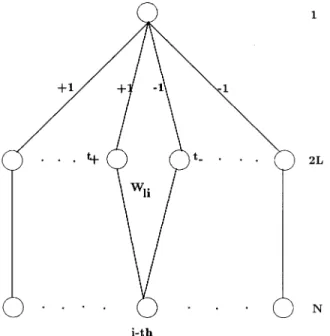
The network’s structure groups the hidden units into pairs, and is shown in Fig. 1. The two weights between each pair of hidden units and the output unit are chosen to be and . The hidden units are allowed to have integer thresholds in
Fig. 1. Two-layer networks with binary weights and integer thresholds.
with being the standard deviation of the input samples and . The reason why is so chosen will become clear when we explain how the constructed network works. The threshold for the output unit is zero.
The weights of the network are constructed using only the samples belonging to Class 1. In particular, the first samples are used to construct the weights of the first pair of hidden units, the second samples are used to obtain the weights for the second pair of hidden units, and so on. The weights ’s connecting the th input with the th
pair of hidden units and are chosen
to be the same for both units, and can be represented as (1)
where , if and , otherwise; and
. The quantity is the th element of the th sample
vector that has been assigned to the
th pair of hidden units. All the elements of sample vectors are drawn independently from the same continuous density function of zero mean and variance . is assumed to have a compact support in , and is symmetric about but bounded away from the origin. That is, only for , where and are constants. Therefore, are independent across all and ; and ’s are independent across all and .
Each of the two hidden units in a pair has a different threshold
(2) where the subscripts and correspond to the two units in a pair with weights and to the output unit. The thresholds are the same for all hidden unit pairs. As will be seen later, the quantity , is approximately the expected
Fig. 2. Two parallel hyperplanes formed by one pair of hidden units.+: samples falling in between the hyperplanes which will have+2 total inputs to the output unit.0: samples falling outside of the hyperplanes which will have0 total inputs to the output unit. The arrows indicate the positive sides of the hyperplanes.
value of the total input to a hidden unit, assuming the sample fed to this unit is chosen from the group of samples assigned to the same pair of hidden units. We will be able to prove later that generating the difference of the thresholds to be a fraction of this quantity will allow both units of this pair to dichotomize correctly the samples assigned to it with high probability.
Fig. 2 gives an intuitive explanation on how the constructed network works given a specific set of samples. Each pair of constructed hidden units can be viewed as two parallel hyperplanes. The amount of separation between these two hyperplanes is characterized by the difference between the two thresholds and it depends on the parameter . One pair of hidden units will contribute to the output unit of the network for samples which fall in between the planes, since they lie on the positive sides of both planes. Each of the samples that has been stored in a particular pair will fall in between the two planes with high probability if the separation between the two planes is properly chosen. Specifically, the separation should be large enough to capture most of the stored samples, but not excessively large since this could allow too many examples from Class 2 to be falsely identified and therefore deteriorate the performance. When the capability of the entire network is considered, the pair of hidden units will have a response to any sample stored in this pair. Since the outputs of all hidden unit pairs are dependent, the outputs due to the rest of the hidden unit pairs can be considered as noise. When the total of hidden unit pairs is not too large, the noise is small, and the output of the network is dominated by the output of the hidden unit pair where the sample is stored. That is, each hidden unit pair can classify the samples stored in this pair to one class, and samples which are not stored in this pair to a different class with a
high probability. How large should be can be characterized through the condition that the probability for all samples to be classified correctly should exceed . That is, if is the total number of incorrectly classified stored samples by the constructed network, an should result in a probability , where is a polynomial in terms of and . Meanwhile, such a constructed network should also classify samples in Class 2 correctly with almost probability assuming is no bigger than the total number of samples in Class 1. This will happen if the total number of hidden unit pairs is not too large compared to , since the larger the , the more likely for a given sample in Class 2 to fall within a pair of parallel hyperplanes, and thus be classified incorrectly.
In the following analysis, three steps are taken to obtain a lower bound for the capacity. First, the probability , that one sample stored in the network is classified incorrectly, is estimated using normal approximations. Similar approxima-tions are then used to estimate . Then
is shown to be approximately a Poisson distribution with a parameter depending on . Conditions on the number of samples stored in each hidden unit pairs, as well as on the total number of hidden unit pairs are then obtained by ensuring the errors due to approximations are small.
B. Probability of Error for a Single Sample
As the first step to obtain a lower bound, we compute which is the probability of incorrect classification of a single random sample stored. Let denote the output of the network when the th sample stored in the th pair is fed through the network. Without loss of generality, we can let and . Since the labels for the stored samples are all , an error occurs if . Then the probability of error for classifying one stored sample can be expressed as
.
Let be the combined contribution due to the th pair of hidden units to the output unit when is fed through the network, i.e.,
(3) Since , can only take two possible values: and
. That is, when
; otherwise, . For the case we consider, and . Then , which belongs to Class 1, is classified incorrectly by the network if for all the hidden unit pairs . That is,
(4)
We observe that depends on
For a fixed
is a summation of independent and identically distributed (i.i.d.) random variables. However, for different , ’s are dependent. In the meantime, the number of hidden unit pairs can also change with respect to the input dimension when goes to infinity. This complicates the analysis. However, using a theorem on normal approximation given in [9], it can be shown in a lemma below that such a probability can be bounded by a probability due to a normal distribution with an additive error term.
Lemma 1: Let with , and
. Assume .1
(5)
where
The proofs of the lemma can be found in Appendix I. It is observed that the quantity
is the normal approximation of the probability of misclassifi-cation of a stored sample, whereas the additive term
is the error due to the normal approximation. This term will go to zero at a rate polynomial in terms of and , as
and go to infinity.
1If 1
C. Probability of Error for All Samples
In this section, we evaluate the probability that all training samples are classified correctly.
Let (6) with (7) and (8)
where is the indicator function, if Event A occurs, and otherwise. Here is the output of the network when the th sample in the set of samples assigned to Class 2 is fed through the network, where . Then and are random variables representing the number of incorrectly classified samples in Class 1 and Class 2, respectively. Likewise, is the total number of incorrectly classified samples. To find a lower bound for the capacity using the constructed network, we need to find an and a condition on so that the probability . To do so, we need to evaluate the probability . In the lemma below, we will first show that
We will then estimate and separately.
Lemma 2: and are independent, i.e.,
(9) Furthermore,
(10)
Moreover, for , we have
(11)
For , , and
(12) The proof of this lemma is given in Appendix II. The quantity
is the normal approximation of the probability of . The added term
is the error due to the normal approximation. This term will go to zero at a rate polynomial in terms of and , when , are large but
with
It should be noted that the constraint, , is needed in order for samples in Class 2 to be classified correctly. Then it remains to find . This is complicated by the fact that the terms in summation (7) are dependent random variables. If the terms were independent, it would be easy to find the corresponding probability. If the dependence among these terms is weak, which is the case we have, under a certain condition, the terms can be treated as being almost independent. This restriction on the number of samples can be obtained through a direct application of a theorem by Stein [11]. Specifically, the theorem shows that under certain conditions is approximately a Poisson distribution.
Theorem 1: Let denote . Then can be
expressed as
(13) Define
(14)
where is chosen arbitrarily from
and
if and
if and .
A single index is used to characterize the double indices just for simplicity, where indicates the
th element in
for and . Then the following inequality holds:
(15)
where is a Poisson distribution: , and with given in (5).
The proof of the theorem is given in Appendix III. Roughly speaking, this theorem indicates that the random variable
has approximately a Poisson distribution if the bound in the above inequality is small. If the random variables ’s were independent, the bound would be on the order of [7]. , however, is an increasing function of as shown in (5). Therefore, for a given and , to make the bound small, cannot be excessively large. When the random variables are weakly dependent, we have a similar situation. That is, an can be found as a function of and , which can result in a similar bound.
Theorem 2: When , we have
(16)
where , . For , and
, we have
(17) where the constants .The proof is given in Appen-dix IV.
Putting (11) and (16) into (9), we have when for
and
(18) where . Such an given in the above theorem yields a lower bound for the capacity as stated in the corollary below.
Corollary 1: If and for
and , a lower bound for the capacity can be obtained as
(19) where is the total number of weights of the network.
It is easy to check that when the aforementioned conditions hold
and
(20)
where . Then by combining (12), (17), and (18), the result will follow by the definition of a lower bound. Intuitively, this corollary indicates that when the number of hidden unit pairs is not too large with respect to , the number of samples stored in each hidden unit pair is , which is on the order of the statistical capacity [8] of a single neuron. In addition, the number of samples each hidden unit pair can store is inversely proportional to which characterizes the separation of two parallel hyperplanes in the pair. The larger the , the larger the separation between two hidden units in a pair, the more likely it is for a sample in Class 2 to fall within two parallel hyperplanes and thus be misclassified. Then the has to bes maller in order for all the stored samples to be classified correctly.
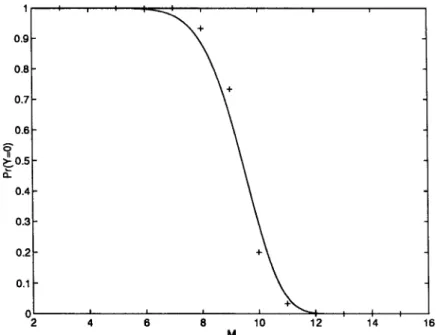
The Monte Carlo simulations are done to compare with the analytical results. Specifically, the probability is estimated for different averaged over 20 runs as given in Fig. 3.2At each run, different numbers of random samples are generated independently from a uniform distribution bounded from zero and assigned randomly to two classes. A two-layer network is then constructed as described in Section III-A using the samples in Class 1. The samples are then fed through the network one by one. A sample is classified correctly by the network if its actual label assigned by the network agrees with its true label. If all the samples are classified correctly by the network, one “successful” run is obtained. The experiment is repeated 20 times. The ratio of the total number of successful runs by the total number of runs gives an estimate for the probability of correct classifications of each . Meanwhile, the probability due to Poisson and normal approximations
is also plotted for comparison. An agreement between the analytical results and the simulation is readily observed.
IV. EVALUATION OF AN UPPERBOUND
As given in the definition, an upper bound is the number of samples whose arbitrary assignments are implemented by any network in the class with a negligible probability. This will happen when the total number of possible binary mappings generated by the networks is no more than a
fraction of all possible dichotomies of the samples, where and are two constants. The total number of binary mappings the networks can possibly generate, however, is no larger than with being a constant. Then for a arbitrarily small, when the number of
samples equals to , the probability
for their arbitrary dichotomies to be implemented by an
network is no larger than .
Therefore, is an upper bound for
the capacity . This quantity is on the order of when and are large. Then is obtained.
2Note that due to the limitation of computer memory,N could not be
Fig. 3. Monte Carlo simulation for the probabilityPr (Y = 0). The solid curve corresponds to the probability obtained in (18). The vertical and horizontal axes arePr (Y = 0) and (M1+ M2)=LN, respectively. The crosses are Monte Carlo simulations for Pr (Y = 0) averaged over 20 runs. In the simulations, the samples are drawn from the uniform distribution in[01; 00:5] and [0:5; 1]. N = 1000, L = 60, M1= M2, = 0:5
It should be noted that since such an upper bound is obtained through counting the total number of binary map-pings possible, it is independent of the distribution of the samples.
V. CONCLUSION
In this work, we have shown that the capacity is lower-bounded by at a certain polynomial rate for , and for any fixed continuous distribution of samples with a compact support and
bounded away from zero as and with
, where is the total number of weights.
We have also shown that as
and for all placements of samples points. Combining both lower and upper bounds, we have
(21) Compared with the capacity of two-layer networks with real weights, the results here show that reducing the accuracy of the weights to just two bits only leads to a loss of capacity by at most a factor of . This gives strong theoretical support to the notion that multilayer networks with binary interconnections are capable of implementing complex functions. The factor difference between the lower and upper bounds for two-layer networks, however, may be due to the limitations of the specific network we use to find a lower bound. A tighter lower bound could perhaps be obtained if a better construction method could be found.
APPENDIX I PROOF OF LEMMA 1
Proof: The proof of the lemma consists of two parts.
In the first part, we describe a general theorem given by [9,
eq. (20.49)] for normal approximation.3We will then use this theorem to estimate in Part II.
Part I. Normal Approximation of Probability of A Sum-mation of Random Vectors: One major result we will use
in this work is normal approximations of joint probabilities of a summation of i.i.d. random vectors with (absolutely) continuous density functions [9]. A similar result was used for lattice distributions in [6].
Let be i.i.d. random vectors in with a continuous density functions, zero mean, and a covariance matrix . is a constant which does not vary with .4Let
(22)
Let be a convex set in . Let be the probability , and be the normal approximation of . That is,
(23) Assume ’s have a finite up to th absolute moment for some
, i.e., for and .
Then
(24) where ’s are the signed measures5
3The main theorem we will be using is the corollary given by [9, eq.
(20.49)]. The corollary is based on [9, Theorem 20.1].
4For the two cases of our interests as will be shown later,k = 1; 2. 5given by [9, eq. (7.3)].
(25) The summation is over all -tuples of positive integers satisfying , and is over all -tuples of nonnegative integral vectors satisfying for . is the th cumulant (or the so-called semi-invariant) of the random vectors ’s. As given in [9, eq. (6.28)], for any nonnegative integral vector
(26) where is a constant depending on only. Meanwhile,
for . Then we have
(27) where is used without loss of generality. This inequality will be used in Part II to estimate .
Part II. Estimating : To estimate , we first consider the difference , where corresponds to the
error event for , and is a normal
approximation to . To obtain the expression for , we first note that since inputs to different hidden unit pairs are uncorrelated,
Each term in the product is the probability of a normal random variable. For , it is easy to check than ,
and . Then (28) where . For (29) (30) (31)
where is the compact support of . Equation (29) is obtained due to the fact that for large
and
can be approximated by and
, respectively. Moreover, when , which is true since has compact support,
through the Taylor expansion. Then (31) is obtained, i.e., (32) Similarly, we can show that the variance of is
(33)
which is approximately for large. Then we have
and
Next, we observe that
(34) where we assume is large enough so that the factor
is neglected. Let . Then
where , and . Since is a
summation of i.i.d. random variables, and the interval is convex, using the normal approximation given in (27) for the dimension of the random vector , and is chosen to be , we can obtain
(35) where
Since is a bounded random variable, . In addition, for any positive integer
(36)
where , and is assumed
to be larger than . Furthermore, it is noticed that the highest
order term6 in given in (25) is [9,
Lemma 7.1], and there are finite terms in the summations.7
Then for and
(37) (38)
For and large
Then the terms due to the signed measures8 are of the smaller order compared to . Therefore, by taking the dominant terms in the bound in (35), we can obtain
(39) where the logarithmic term in
is neglected, since it is of the smaller order. Putting (39) into (34), we have
(40) i.e.,
(41) It should be noted that due to the use of inequality (34) the resulting bound is not very tight. However, as will be seen later, such an error estimate is good enough to obtain a satisfactory lower bound for the capacity. Q.E.D.
6in the power ofD 7
i!’s are on the order of O(1) as well.
8which are in the order ofO p 1
N(NL)
APPENDIX II PROOF OF LEMMA 2
The proof of the lemma also consists of two parts. In Part I, we will prove (9) and (10) are true. In Part II, we will derive (11) and (12).
Part I: First, we show that and are independent. Consider the inputs to each of two units in the first hidden unit pair when the samples in Class 1 and in Class 2 are fed through the network. Without loss of the generality, we can choose . Then we have
(42) and
(43)
where ’s are the elements of for . is
the total input to each of the two units in the first hidden unit pair when a sample assigned to Class 2 is fed through the network. Since the terms with different subscripts are independent, which is easy to check, we only need to show the independence of the two terms with the same subscript in
the above two summations. Let and .
Then for any
(44)
(45)
(46) Here (45) is obtained from (44) due to the independence of the samples; while (46) is derived from (45) since
is independent of and is symmetrically distributed,
i.e., . On the other hand,
(47)
(48) Therefore,
This approach can be extended to all variables in sum-mations (42) and (43) to show the mutual independence of all terms. Then and are independent. Similarly, we can show the independence for the other pairs of hidden units.
Therefore, and are independent. The
mutual independence of and for all
, , and can be shown using a
similar approach extended to multiple variables. Then and can be shown to be independent.
Similarly, we can show that ’s for are also mutually independent. Then
(49)
Part II: We use normal approximation given in Part I of
Appendix I to obtain a bound for . Let be the total output of the th hidden unit pair when is fed through the network. Let . Since ’s are uncorrelated, it is easy to obtain that the normal approximation
of as
(50) Then for
(51) where is the complement of . The last inequality is obtained using the union bound. Furthermore,
using the normal approximation given in (27) and similar derivations from (34) and (39), we have, for
and large
(52) where the terms due to the signed measures are neglected, since they are of the smaller order. Putting (52) into (51), we can obtain (53) Therefore, (54) For , , and (55) where . Q.E.D. APPENDIX III PROOF OF THEOREM 1
This theorem is a direct application of a theorem by Stein [11] which can be described as follows.
Theorem 3. Stein’s Original Theorem: Let
(56) where ’s are Bernoulli random variables taking values and , and . is the total number of random variables.
Let . Define
(57)
such that the distribution of is the same as the conditional distribution of given . Then
(58)
where , and .
The proof of Stein’s theorem can be found in [11]. To apply Stein’s theorem to our case, we define and as given in (13) and (14), respectively. Then corresponds to . and correspond to and , respectively. In addition, since ’s are exchangeable random variables [3], the distribution of is the same as the conditional distribution
of given for any by the definition of
. Then the result given by (58) applies to our case directly. Q.E.D. APPENDIX IV
PROOF OF THEOREM 2
There are two parts in the proof. In Part I, we will derive a bound for the Poisson approximation. In Part II, we will estimate the joint probabilities needed in the bound using normal approximations.
Part I: We will start with a brief outline of the proof. Based
on Stein’s theorem, to show that the Poisson approximation holds, it suffices to show that the bound given in (15) is asymptotically small for large (but ) when the number of stored samples at each pair grows at certain rate in terms of and . To do that, we will first obtain a new bound for (15) through Jensen’s inequality. Each individual term in the new bound will be further bounded using Schwartz’s inequality to simplify the derivations. Finally, normal approximations will be used to estimate the joint
probabilities in each term. The detailed proof is given as follows.
Due to the fact that ’s and are exchangeable random variables
for all Then
(59) where . By Jensen’s inequality,
If which will be the case we consider, to show the Poisson approximation holds, we only need to find conditions on so that is asymptotically
small for large and . , however, can
be expressed as (60) where (61) (62) (63) (64) (65) (66) Due to the fact that ’s are exchangeable random variables, the subindices in (62)–(66) are chosen without loss of general-ity. To further simplify the derivations, Schwartz’s inequality is used to obtain
(67)
where .
Then by taking the dominant terms for large and , we can obtain (68) (69) (70) (71) (72)
Therefore, only two expectations and
need to be evaluated to estimate the bound. (73) where the identities have been used for the indicator variables:
and . Since (74) (75) we have (76) Similarly, we have (77) Then to estimate the error bound for the Poisson approxima-tion, we need to estimate the joint probabilities,
and .
Part II: To estimate these probabilities, we use the theorem
for the normal approximation given in Part I of Appendix I. Let the joint error event , i.e.,
Let
Then using the similar inequality as that given in (34), we have
(78) where is the normal approximation of
, and is the normal approximation of . Let
and
where the mean and the variance are
given in (32) and (33), respectively. The event corresponds to the random vector falling into the four convex regions, ’s, for , where
Then
(79)
Using the normal approximation for ’s and taking , we have
(80) where
is the covariance matrix of
(81)
and . , where
(82) with being the probability density function of two jointly normal random variables, i.e.,
(83)
To estimate , we note that can be
expanded as [6]
(84) where
for
Then for and large, by putting (84) into (82), we have
(85) where is a smaller order term. In addition, it is easy to
check that all ’s for and are
uncorrelated, we have
(86)
To estimate the bound in the inequality given in (80), we use similar derivations as given in Part II of Appendix I. Specifi-cally, it is noted that the derivative in (80) can be bounded (for large) through the inequality
(87) Since the highest order term is of the order , and is chosen to be , we have
(88) Furthermore, since and are bounded,
for any finite . In addition, there are finite terms in the summations given in (80). Then by taking the dominant term, we have
(89) (90) For
and
Then the summation given in (89) is of smaller order compared with . Therefore, taking the dominant terms, we have
(91) Finally, using the triangle inequality, we can have
(92) From (5), we can easily derive that
(93) Combining (92) and (93) together, we have
(94) Using similar derivations, we can obtain
Furthermore,
Since the bound for dominates all bounds, when
with , and , we have
(96)
for , .9 Q.E.D.
ACKNOWLEDGMENT
This paper is dedicated to the memory of Prof. Ed Posner. The authors wish to thank anonymous referees and the associate editor for pointing out an error in the previous manuscript and for their valuable comments.
9It can easily be shown thatLMP
e1= o(1) is also satisfied.
REFERENCES
[1] E. Baum, “On the capacity of multilayer perceptron,” J. Complexity, 1988.
[2] L. Neiberg and D. Casasent, “High-capacity neural networks on nonideal hardware,” Appl. Opt., vol. 33, no. 32, pp. 7665–7675, Nov. 1995. [3] Y. S. Chow and H. Teicher, Probability Theory: Independence,
Inter-changeability, Martingales. New York: Springer-Verlag, 1988. [4] T. M. Cover, “Capacity problems for linear machines,” in Pattern
Recognition, L. Karnal, Ed. Washington, DC: Thompson, 1968, pp. 283–289.
[5] H. Cramer, Mathematical Methods of Statistics. Princeton, NJ: Prince-ton Univ. Press, 1946.
[6] A. Kuh and B. W. Dickinson, “Information capacity of associative memory,” IEEE Trans. Inform. Theory, vol. 35, pp. 59–68, Jan. 1989. [7] L. Le Cam, “An approximation theorem for the Poisson binomial
distribution,” Pacific J. Math., vol. 10, pp. 1181–1197, 1960. [8] R. J. McEliece, E. C. Posner, E. R. Rodemich, and S. S. Venkatesh,
“The capacity of the Hopfield associative memory,” IEEE Trans. Inform. Theory, vol. IT-33, pp. 461–482, July 1987.
[9] R. N. Bhattacharya and R. R. Rao, Normal Approximation and Asymp-totic Expansions. New York: Wiley, 1975.
[10] G. Dundar and K. Rose, “The effects of quantization on multilayer neural networks,” IEEE Trans. Neural Networks, vol. 6, pp. 1446–1451, Nov. 1995.
[11] C. Stein, “Approximate computation of expectations,” in Inst. Math. Statist. Lecture Notes, Monograph Ser., vol. 7, Hayway, CA, 1988. [12] S. Venkatesh, “Directed drift: A new linear threshold algorithm for
learning binary weights on-line,” J. Comput. Syst. Sci., vol. 46, no. 2, pp. 198–217, 1993.