CDO Pricing with Copulae

SFB 649 Discussion Paper 2009-013

CDO Pricing with Copulae

Barbara Choro

ś

*

Wolfgang Härdle*

Ostap Okhrin*

*Humboldt-Universität zu Berlin, Germany

This research was supported by the Deutsche

Forschungsgemeinschaft through the SFB 649 "Economic Risk". http://sfb649.wiwi.hu-berlin.de

ISSN 1860-5664

SFB 649, Humboldt-Universität zu Berlin Spandauer Straße 1, D-10178 Berlin

S

FB

6

4

9

E

C

O

N

O

M

I

C

R

I

S

K

B

E

R

L

I

N

CDO Pricing with Copulae

∗

Barbara Choro´s

, Wolfgang H¨

ardle, Ostap Okhrin

March 5, 2009

Abstract

Modeling the portfolio credit risk is one of the crucial issues of the last years in the financial problems. We propose the valuation model of Collateralized Debt Obligations based on a one- and two-parameter copula and default intensities esti-mated from market data. The presented method is used to reproduce the spreads of the iTraxx Europe tranches. The two-parameter model incorporates the fact that the risky assets of the CDO pool are chosen from six different industry sec-tors. The dependency among the assets from the same group is described with the higher value of the copula parameter, otherwise the lower value of the parameter is ascribed. Our approach outperforms the standard market pricing procedure based on the Gaussian distribution.

Keywords: CDO, CDS, multifactor models, multivariate distributions, Copulae,

correlation smile.

JEL classification: C14, G12, G13

∗_{The financial support from the Deutsche Forschungsgemeinschaft via SFB 649 “Okonomisches}

Risiko”, Humboldt-Universit¨at zu Berlin is gratefully acknowledged.

†_{Corresponding author. CASE - Center for Applied Statistics and Economics, Institute for Statistics}

and Econometrics of Humboldt-Universit¨at zu Berlin, Spandauer Straße 1, 10178 Berlin, Germany. Email: [email protected].

1

Collateralized Debt Obligations

The collateralized debt obligation (CDO) is a financial instrument that enables securi-tization of a large portfolio of assets like loans, bonds or credit default swaps (CDS). The portfolio’s risk is sliced into tranches of increasing seniority and then sold separately. Investors, according to their risk preferences, buy default risk of the underlying pool in exchange for a fee. Each tranche has specified priority of bearing claims and of receiving periodic payments.

A CDO transaction has two sides – asset and liability – linked by cash flows. The asset side refers to the underlying reference portfolio where the liability side consists of securities issued by an issuer, which often is a special purpose vehicle (SPV). An SPV is a company created by an owner of a pool specially for the transaction to insulate investors from the credit risk of the CDO originator. An originating institution, usually a bank, sells assets to an SPV which issues in the market structured notes backed by the portfolio on its balance. For further details refer to Bluhm & Overbeck (2006).

Each CDO tranche is defined by the detachment (lj) and attachment (uj) points which

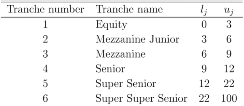
are the percentages of the portfolio losses. Table 1 presents the classical tranching taken from the iTraxx index. This example shows that the most subordinated tranche, called equity or residual tranche, bears the first 3% losses of the portfolio nominal. The equity tranche investors are also payed an upfront fee. If losses constitute 5% of the collateral notional, the equity investors carry the first 3% (thus loosing all their investment), and the next 2% are covered by those who invested in the mezzanine junior tranche. The tranches called senior carry the lowest risk. The super super senior suffers only if the total collateral portfolio loss exceeds 22% of its notional value.

Tranche number Tranche name lj uj

1 Equity 0 3

2 Mezzanine Junior 3 6 3 Mezzanine 6 9

4 Senior 9 12

5 Super Senior 12 22 6 Super Super Senior 22 100

Table 1: Example of a CDO tranche structure, iTraxx. Attachment points given in percent.

Each loss that is covered reduces the notional on which the payments are based and also reduces the value of the periodic fee. After each default the seller of the protection makes a payment equal to the loss to the protection buyer. When the portfolio losses exceed the detachment point no notional remains and no payment is made.

2

Defaults, Joint Defaults and Copulae

The prices of the CDO tranches depend on the joint random behavior of the assets in the underlying pool, more precisely, on their likelihood of joint defaults. Synthetic CDOs, considered in the empirical part of this study, are backed by a portfolio ofdCDS. A CDS is an insurance contract between two counterparties covering the risk that a specified credit defaults. The final result of the CDO calibration depends strongly on the evaluation of the risk of each underlying CDS contracts. The individual default probabilities of the reference entities are calculated within the framework of the intensity model.

Assume the existence of a filtered probability space (Ω,F,P) with a probability measure P. Letτi be a positive random variable representing the time of default ofith CDS,i= 1,

. . . , d, with a distribution function Fi. The term structure of default probability (the

credit curve) is defined as pi(t) = P(τi ≤ t) = Fi(t) and represents the probability that

the obligor defaults within the time interval [0, t]. In this approach the obligor’s default is modeled as the time until the first jump of a Poisson process. The unconditional default probabilities are related to the intensity function λi(t) by the equality:

pi(t) = 1−exp − Z t 0 λi(u)du ,

where the corresponding survival probability term structure is given by

¯

pi(t) = 1−pi(t) = P(τi > t).

In the simulation study we consider that the ith obligor survives until t if and only if

Ui ≤p¯i(t), where Ui is a random variable uniformly distributed on [0,1] called a trigger.

The difficulty in modeling the default risk of the CDO lies in finding the relation between default timesτ1, . . . ,τd. The main task consist of determining the joint distribution for the

stopping times such that the marginal distributions are the credit curves. Multivariate copula functions provide a convenient way to specify the joint distribution with given margins.

A copula can be defined as an arbitrary distribution function on [0,1]d _{with uniform}

margins. The usefulness of copulae comes from Sklar’s theorem which shows that a d -dimensional distribution functionF can be expressed in terms of a copula and the marginal distribution functionsF1, . . . , Fd

F(x1, . . . , xd) =C{F1(x1), . . . , Fd(xd)}.

A survey over the mathematical foundations and properties of copulae is given by Nelsen (2006).

The copula C of the triggers U1, . . . , Ud describes the complete dependence structure of

the default times. The time to default variable

is calculated as the first time when the process ¯pi(t) reaches the level of the trigger variable

Ui, see Sch¨onbucher (2003). In this study we assume the constant intensities for which

the default times are simply computed as τi =−lnUi/λi.

The choice of the appropriate copula plays a crucial role in the final results. The selected function should represent desirable tail properties and the algorithm of generating the random numbers from it need to be known. The model can contain up to d(d−1)/2 parameters if the dependency is assumed to be Gaussian or t and only one parameter for a simple Archimedean copula.

To handle the dimensionality in modeling the iTraxx data we apply the hierarchical Archimedean copulae (HAC), the generalization of the multivariate Archimedean copulae. The profound study of HAC is provided by Okhrin, Okhrin & Schmid (2008). We use the fact that the CDS from the pool represent six industry sectors: consumer, financial, technology-media-telecommunications (TMT), industrials, energy and auto. The number of swaps in the groups is 30, 25, 20, 20, 20, 10 respectively. Therefore we can construct the seven-parameter model in which the dependency in each group is described with a distinct one-parameter copula and the relations outside the groups are characterized with additional, seventh parameter. Another simplification consist of integrating the industry sectors, for example, into two groups and can be represented using the correlation matrix as: R=                                 1 · · · ρ2 . .. ρ2 · · · 1 ρ1 · · · · .. . ρ1 · · · ρ1 .. . .. . ρ1 · · · ρ1 .. . .. . 1 · · · ρ2 . .. ρ2 · · · 1 . .. 1 · · · ρ3 . .. ρ3 · · · 1 .. . .. . ρ1 · · · ρ1 .. . .. . ρ1 · · · · ρ1 .. . · · · ρ1 1 · · · ρ3 . .. ρ3 · · · 1                                 (1)

When one deals with copulae, the correlation termρmeans not Pearson linear correlation, but a rank based correlation, like Kendall’s τ or Spearman’s ρs. If in the matrix above

ρ2 =ρ3andρ1 6=ρ2, then the model comprises the industry factor which assumes different

inter- and intra-industry correlation. Using the partially nested HAC we first model the dependency in the group with an Archimedean copula C2 and then we join all groups

with another Archimedean copula C1. The applied HAC has the following form:

C(u1, . . . , ud) = C1{C2(u1, . . . , um1), C2(um1+1, . . . , um1+m2), . . . , C2(um1+...+m5+1, . . . , ud)},

(2) where mk,k = 1, . . . , 6, indicates a number of the companies in kth industry sector.

3

Valuation of CDO

Consider a CDO ofJ tranches. The portfolio loss process

L(t) = 1 d d X i=1 (1−Ri)Γi,t, t ∈[0, T] (3)

is the average of the obligors’ loss variables defined as Γi(t) =I(τi ≤t),i= 1, . . . , d. The

loss of the tranchej = 1, . . . , J, at timet is determined by its attachment points and the portfolio loss: Lj(t) = min{max(0, Lt−lj);uj−lj} =    0, Lt< lj, Lt−lj, lj ≤Lt ≤uj, uj−lj, Lt> uj.

In the CDO transaction, the protection seller receives insurance payments for which he obliges himself to cover losses affecting his tranche. The present value of the sum of contingent payments done upon credit events is called the protection leg. The premium leg refers to the present value of the sum of fee payments made by the protection buyer during the life of the contract. The payments connected with tranche j at time t are worked out from the outstanding notional of the form:

Fj(t) = (uj−lj)−Lj(t), j = 1, . . . , J.

The buyer and the seller settle the cash obligations at predefined dates, usually once per quarter, until maturityT of the contract or until Fj = 0. The credit event can happen at

any time but to get a close form solution we make a slightly simplifying assumption that all defaults occur in the middle of a payment period. The premium legP Lj is then based

on the expected average of outstanding notionals from the two nearest payment days:

P Lj(t0) =

T

X

t=t1

β(t0, t)sj(t0)∆tE{Fj(t) +Fj(t−∆t)}M/2, j = 2, . . . , J,

wheret1is the date of the first payment after the trade is made, ∆tis a fraction of the year between t and the nearest preceding payment day. The sum is taken over all scheduled payment days. All settlements are discounted to the time pointt0 using the compounded

The most subordinated tranche is priced differently than the other tranches. It pays an upfront fee once, at the inception of the trade and a fixed coupon of 500 bps during the life of the contract. The upfront payment, denoted by α, is expressed in percent and is quoted in the market. The premium leg of the residual tranche is defined as:

P L1(t0) =α(t0)(u1−l1)M+

T

X

t=t1

β(t0, t)500∆tE{F1(t) +F1(t−∆t)}M/2.

The protection leg DLj for all the tranches is calculated as follows:

DLj(t0) =

T

X

t=t1

β(t0, t)E{Lj(t)−Lj(t−∆t)}M, j= 1, . . . , J. (4)

The premium sj of the tranche j is chosen in such a way that the market value of the

contract is zero, which means that the both premium and protection legs are equal:

P Lj(t0) = DLj(t0).

This leads to the solution:

sj(t0) = PT t=t1β(t0, t)E{Lj(t)−Lj(t−∆t)} PT t=t1β(t0, t)∆tE{Fj(t) +Fj(t−∆t)}/2 , for j = 2, . . . , J. (5)

If we denote the denominator of the formula (5) by

P L∗_j(t0) =

T

X

t=t1

β(t0, t)∆tE{Fj(t) +Fj(t−∆t)}/2, (6)

we get the fair spread of the form:

sj(t0) =

DLj(t0) P L∗_j(t0)

for j = 2, . . . , J.

For the equity tranche the upfront payment is equal to:

α(t0) = 100 u1−l1 T X t=t0 [β(t, t0)E{L1(t)−L1(t−∆t)} −500∆tE{F1(t) +F1(t−∆t)}/2].

The CDO spreads sj(t0),j = 2, . . . , J, and the upfront feeα(t0) are constantly observed

in the market. Our aim is to find a model that calculates the prices which are close to the real values and which do not result in a formation of the implied correlation smile.

4

Empirical Results

The empirical research of this study was performed using the iTraxx Euro index series 8 with the maturity of 5 years. The series 8 was issued on 20th September 2007 and expires

on 20th December 2012. The computations were carried out for the constant interest rate

r = 0.03 and the constant recovery rate R = 0.4 on day t0: 22nd October 2007. We considered all d = 125 underlying CDS contracts and J = 5 CDO tranches, from the equity to the super senior.

We start with estimating the univariate distributions of each time to default variable τi,

i= 1, . . . , 125, in the framework of the reduced form model. The intensity for which the fair spread of a CDS matches the market spread is implied from the CDS pricing model using a bisection method.

Afterwards we generate 106 _{times a vector of trigger variables (U}

1, . . . , Ud) ∼ C from

different dependency structure. The copulae taken into consideration were the one- and parameter Gaussian and the one- and parameter Gumbel. The applied two-parameter Gumbel copula is a HAC given by (2). The method of sampling from a nested Gumbel copula was taken from McNeil (2008).

The Monte Carlo samples of the default times allow for calculating the portfolio loss process L(t) using (3) and then for getting the default legs DLj(t0) defined in (4) and P L∗_j(t0) from (6). The expected values in these formulae are calculated as the sample averages over 106 values. We denote the sample default leg with DLd_j(t₀) and the sample

premium leg withP Lc_j(t₀). Finally, the model spread is computed as:

sc_j(t0) = d DLj(t0) c P L∗_j(t0) for j = 1, . . . , J.

We now show how to find the copula parameters that reproduce the true prices. The main idea of the calibration is to minimize the relative deviations from the market spreads sm j D def= J X j=1 |sc_j −sm_j | sm j →min.

As the first tranche doesn’t quote spread in the market, we don’t observesm

1 . To allow for

the comparison of the first tranche with other tranches we transform the equity tranche that gives the upfront fee and the constant running spread into the tranche with changing running spread and no upfront fee. The equivalent equity tranche has the following spread

sm₁ (t0) = αm(t0)(u1−l1)100/P L∗_j(t) + 500,

where αm_(t

0) is the market upfront fee.

In case of the one-parameter copulae the result is attained with the bisection method. For the optimal copula parameter the objective function D satisfies D < ε, where ε is a small enough level.

In the estimation of the two-factor models we first assume that the unknown parameters are equal, ρ1 = ρ2. For the starting point we take the outcome of the one-parameter

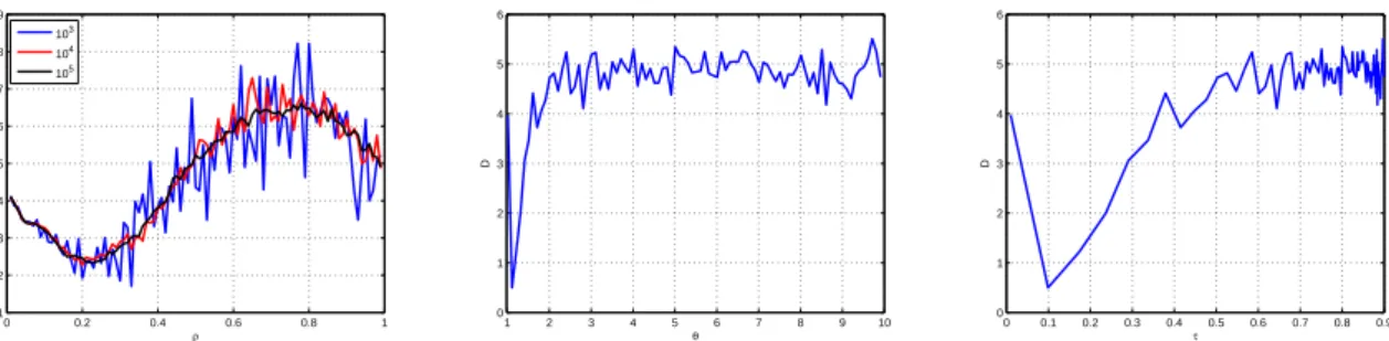
0 0.2 0.4 0.6 0.8 1 1 2 3 4 5 6 7 8 9 ρ D 103 104 105 1 2 3 4 5 6 7 8 9 10 0 1 2 3 4 5 6 θ D 0 0.1 0.2 0.3 0.4 0.5 0.6 0.7 0.8 0.9 0 1 2 3 4 5 6 τ D

Figure 1: Calibration of the one-factor models. Data from 20071022,RR= 0.4,r = 0.03,

N = 104_.

the parameters. We go along the path by changing ρ1 and ρ2 where the measure D is

minimized. Asρ2 measures the dependence within the industry sector it is never smaller

than ρ1. Moreover, the condition ρ1 ≤ ρ2 guarantees that the correlation matrix (1) is

positive-definite and the function C is a proper copula, see McNeil & Neˇslehov´a (2008). Thus the grid has a triangular shape. We start from the diagonal of the grid and calculate the function D in three points equally distant from the origin. The considered points lie to the left, to the left diagonally and up. We choose this direction that gives the smallest value ofD.

The left panel of Figure 1 exhibits the measureDcalculated for one-factor Gaussian model for ρ∈(0,1). We see that the final result is very sensitive to the number of Monte Carlo simulations. The middle and the right panel of Figure 1 depicts the measure D for the one-factor Gumbel model forθ and the Kendall’sτ. The Kendall’s τ can be conveniently computed in case of the Gumbel copula via the identityτ = 1−1/θ. For both parameters we obtain the unique solution.

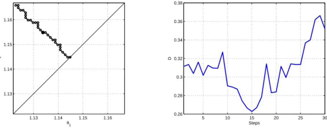
The calibration of the two-factor model with the Gaussian dependency structure is il-lustrated in Figure 2 and in the left panel of Figure 4. The solution of the one-factor Gaussian model is marked with a small black dot on the diagonal. Other black points represent the path where the objective function has its local minimum. The global mini-mum is selected by the comparison of all local ones and is marked with a bold dot. The same investigation is carried out for the two-factor Gumbel copula model. The results are depicted in Figure 3. In both cases the final solution was found in not more than 15 steps. The right panels of Figure 2 and 3 illustrate that after the minimum is localised, the objective functions have increasing trends and we do not expect the global minimum in the next steps.

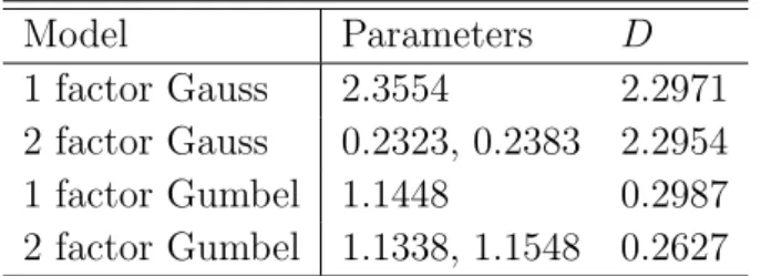
Table 2 exhibits the results of the estimation of four models. We see that the Gumbel copula models provide much precise fit to iTraxx market data than the Gaussian cop-ula models. In addition we find that two-factor models outperform these with only one parameter. However the two parameters seems to be very close to each other and the improvement of the two-factor model compared to the one-factor model for both depen-dency structure is small. The right panel of Figure 4 shows that the Gumbel copula models satisfactorily reproduces the market spreads.

0.1 0.2 0.3 0.4 0.5 0.1 0.2 0.3 0.4 0.5 ρ1 ρ2 5 10 15 20 25 30 2.295 2.3 2.305 2.31 2.315 2.32 2.325 2.33 2.335 Steps D

Figure 2: Calibration of the two-factor Gaussian model. Steps of the algorithm, data from 20071022,RR= 0.4,r = 0.03, N = 106_. 1.13 1.14 1.15 1.16 1.13 1.14 1.15 1.16 θ₁ θ2 5 10 15 20 25 30 0.26 0.28 0.3 0.32 0.34 0.36 0.38 Steps D

Figure 3: Calibration of the two-factor Gumbel model. Steps of the algorithm, data from 20071022, RR= 0.4, r= 0.03, N = 106. ρ₁ ρ2 0.2 0.4 0.6 0.8 0.1 0.2 0.3 0.4 0.5 0.6 0.7 0.8 0.9 2 3 4 5 20 40 60 80 100 120 140 Tranches Spread Market 1 Gumbel 2 Gumbel

Figure 4: Calibration of the two-factor Gaussian model (left panel). Comparison of the results of the Gumbel copula models (right panel).

Model Parameters D

1 factor Gauss 2.3554 2.2971 2 factor Gauss 0.2323, 0.2383 2.2954 1 factor Gumbel 1.1448 0.2987 2 factor Gumbel 1.1338, 1.1548 0.2627

Table 2: Comparison of the CDO pricing copula models.

References

Bluhm, C. & Overbeck, L. (2006). Structured Credit Portfolio Analysis, Baskets and CDOs, CRC Press LLC.

McNeil, A. J. (2008). Sampling nested Archimedean copulas,Journal Statistical

Compu-tation and Simulation . forthcoming.

McNeil, A. J. & Neˇslehov´a, J. (2008). Multivariate Archimedean copulas, d-monotone functions and l1 norm symmetric distributions, Annals of Statistics . forthcoming.

Nelsen, R. B. (2006). An Introduction to Copulas, Springer Verlag, New York.

Okhrin, O., Okhrin, Y. & Schmid, W. (2008). On the structure and estimation of hierar-chical Archimedean copulas, under revision .

Sch¨onbucher, P. (2003). Credit Derivatives Pricing Models: Model, Pricing and

SFB 649 Discussion Paper Series 2009

For a complete list of Discussion Papers published by the SFB 649, please visit http://sfb649.wiwi.hu-berlin.de.

001 "Implied Market Price of Weather Risk" by Wolfgang Härdle and Brenda López Cabrera, January 2009.

002 "On the Systemic Nature of Weather Risk" by Guenther Filler, Martin Odening, Ostap Okhrin and Wei Xu, January 2009.

003 "Localized Realized Volatility Modelling" by Ying Chen, Wolfgang Karl Härdle and Uta Pigorsch, January 2009.

004 "New recipes for estimating default intensities" by Alexander Baranovski, Carsten von Lieres and André Wilch, January 2009.

005 "Panel Cointegration Testing in the Presence of a Time Trend" by Bernd Droge and Deniz Dilan Karaman Örsal, January 2009.

006 "Regulatory Risk under Optimal Incentive Regulation" by Roland Strausz, January 2009.

007 "Combination of multivariate volatility forecasts" by Alessandra Amendola and Giuseppe Storti, January 2009.

008 "Mortality modeling: Lee-Carter and the macroeconomy" by Katja Hanewald, January 2009.

009 "Stochastic Population Forecast for Germany and its Consequence for the German Pension System" by Wolfgang Härdle and Alena Mysickova, February 2009.

010 "A Microeconomic Explanation of the EPK Paradox" by Wolfgang Härdle, Volker Krätschmer and Rouslan Moro, February 2009.

011 "Defending Against Speculative Attacks" by Tijmen Daniëls, Henk Jager and Franc Klaassen, February 2009.

012 "On the Existence of the Moments of the Asymptotic Trace Statistic" by Deniz Dilan Karaman Örsal and Bernd Droge, February 2009.

013 "CDO Pricing with Copulae" by Barbara Choros, Wolfgang Härdle and Ostap Okhrin, March 2009.

SFB 649, Spandauer Straße 1, D-10178 Berlin http://sfb649.wiwi.hu-berlin.de