Two-Sided Matching and Spread Determinants in the Loan
Market
Jiawei Chen
∗August 24, 2006
Abstract
Empirical work on bank loans typically regresses loan spreads (markups of loan inter-est rates over a benchmark rate) on observed characteristics of banks,firms, and loans. The estimation is problematic when some of these characteristics are only partially ob-served and the matching of banks and firms is endogenously determined because they prefer partners that have higher quality. We study the U.S. bank loan market with a two-sided matching model to control for the endogenous matching, and obtain Bayesian inference using a Gibbs sampling algorithm with data augmentation. Wefind evidence of positive assortative matching of sizes, explained by similar relationships between quality and size on both sides of the market. Banks’ risk andfirms’ risk are important factors in their quality. Controlling for the endogenous matching has a strong impact on estimated coefficients in the loan spread equation.
KEYWORDS: Two-Sided Matching, Loan Spread, Bayesian Inference, Gibbs Sam-pling with Data Augmentation
1
Introduction
Bank loans play a unique role in corporatefinancing. They are important not only for small busi-nesses, which often lack access to public debt markets, but also for large corporations, which depend on them as a reliable source of liquidity helping to insulate them from market shocks (Saidenberg and Strahan, 1999; James and Smith, 2000). Furthermore, bank lending is an important conduit for monetary policy and is closely linked to investment and macroeconomic activity (Kashyap and ∗Department of Economics, 3151 Social Science Plaza, University of California, Irvine, CA 92697-5100. E-mail: [email protected]. I thank Joseph Harrington, Ivan Jeliazkov, Ali Khan, Robert Moffitt, Matthew Shum, Tiemen Woutersen, and seminar participants at Brown, Iowa, Johns Hopkins, St. Louis Fed, UC-Irvine, USC, and Williams College for helpful comments and suggestions. I am grateful for the support from the Carl Christ Fellowship.
Stein 1994). Not surprisingly, empirical researchers have long been interested in the pricing of bank loans. For example, loan spreads (markups of loan interest rates over a benchmark rate) are regressed on characteristics of banks, firms, and loans to examine the relationship between collateral and risk infinancial contracting (Berger and Udell, 1990), and to provide evidence of the bank lending channel of monetary transmission (Hubbard, Kuttner, and Palia, 2002). However, the non-randomness of the bank-firm pairs in the loan samples is typically ignored. In this paper, we argue that banks and firms prefer to match with partners that have higher quality, so banks choosefirms,firms choose banks, and the matching outcome is endogenously determined. We show that because of the endogeneity, the regressors in the loan spread equation are correlated with the error term, so OLS estimation is problematic. We develop a two-sided matching model to take into account the endogenous matching, and show that controlling for the endogenous matching has a strong impact on the estimates.
Both firms and banks have strong economic incentives to choose their partners. When a bank lends to a firm, the bank not only supplies credit to the firm but also provides monitoring, expert advice, and endorsement based on reputation (e.g. Diamond, 1984 and 1991). Empirical evidence suggests that those “by-products” are important for firms. For instance, Billet, Flannery and Garfinkel (1995) and Johnson (1997) show that banks’ monitoring ability and reputation have significant positive effects on borrowers’ performance in the stock market.
The size of a bank–the amount of its total assets–also plays an important role in firms’ choices. First, a larger bank is likely to have better diversified assets and a lower risk, making it more attractive to firms. Second, the small size of a bank may place a constraint on its lending, which is undesirable for a borrowing firm, since its subsequent loan requests could be denied and it might have tofind a new lender and pay a switching cost. Third, large banks usually have more organizational layers and face more severe information distortion problems than small banks, so they are generally less effective in processing and communicating borrower information, making them less able to provide valuable client-specific monitoring and expert advice. Fourth, Brickley, Linck and Smith (2003) observe that employees in small to medium-sized banks own higher percentages of their banks’ stocks than employees in large banks. As a result the loan officers in small to medium-sized banks have stronger incentives and will devote more effort to collecting and processing borrower information, which helps the banks better serve their clients. Thus the size of a bank has multiple effects on its quality perceived by firms and those effects operate in opposite directions. Which bank size is most attractive is determined by the net effect.
Banks’ characteristics affect how much benefit borrowingfirms will receive, sofirms prefer banks that are better in those characteristics, e.g., banks with higher monitoring ability, better reputation, suitable size, and so on. Banks are ranked by firms according to a composite quality index that combines those characteristics.
Now consider banks’ choices. In making their lending decisions, loan officers in a bank screen the applicants (firms) and provide loans only to those who are considered creditworthy. Firms with lower leverage ratios (total debt/total assets) or higher current ratios (current assets/current liabilities) are usually considered less risky and more creditworthy. Larger firms also have an advantage here, because they generally have higher repaying ability and better diversified assets, and are more likely to have well-documented track records and lower information costs.
However, the large size of a firm also has negative effects on its attractiveness. Because larger
firms have stronger financial needs, the loan made to a larger firm usually has a larger amount and accounts for a higher percentage of the bank’s assets, thus reducing the bank’s diversification. Since banks prefer well diversified portfolios, the large size of a borrowing firm may be considered unattractive. In addition, lending to a large firm means that the bank’s control over the firm’s investment decisions will be relatively small, which is undesirable.1 Therefore, the size of a firm also has multiple effects on its quality perceived by banks, and whichfirm size is most attractive depends on the relative magnitudes of those effects. Firms are ranked by banks according to a composite quality index that combines firms’ characteristics, such as their risks and their sizes.
The above analysis shows that there is endogenous two-sided matching in the loan market: banks choose firms, firms choose banks, and they all prefer partners that have higher quality. Consequently, firms with higher quality tend to match with banks with higher quality, and vice versa.
In our model banks’ andfirms’ quality are multidimensional, but to illustrate the implications of the endogenous matching, we assume for a moment that a bank’s quality is solely determined by its liquidity risk, and that afirm’s quality is solely determined by its information costs. Further assume that banks’ liquidity risk, firms’ information costs, and non-price loan characteristics such as maturity and loan size are determinants of loan spreads. The spread equation is:
rij =α0+κLi+λIj+Nij0 α3+νij, νij ∼N(0, σ2ν), (1)
where rij is the loan spread if bank i lends to firm j, Li is bank i’s liquidity risk, Ij is firm j’s 1See Rajan (1992) for a discussion on banks’ control over borrowers’ investment decisions.
information costs, andNij is the non-price loan characteristics.
Liquidity risk and information costs are not perfectly observed, and the bank’s ratio of cash to total assets and thefirm’s ratio of property, plant, and equipment (PP&E) to total assets are used as their proxies, respectively. Assume
Li=ρCi+ηi, ηi ∼N(0, σ2η), and
Ij =σPj+δj, δj ∼N(0, σ2δ),
where Ci is banki’s ratio of cash to total assets, and Pj isfirm j’s ratio of PP&E to total assets.
Now equation (1) becomes
rij = α0+κ(ρCi+ηi) +λ(σPj +δj) +Nij0 α3+νij
= α0+κρCi+λσPj+Nij0 α3+κηi+λδj+νij. (2)
Note that the error term contains ηi andδj, the unobserved quality. Because of the endogenous
matching, the characteristics of the partner of a bank or afirm are correlated with the bank or the
firm’s unobserved quality. As a result, the regressors in the spread equation are correlated with the error term, so OLS estimation of the equation is problematic.2 Furthermore, since any variable that influences the matching affects the error term through the unobserved quality, the method of instrumental variables (IV) is not applicable here.
To take into account the endogenous matching, a many-to-one two-sided matching model in the loan market is developed and estimated. The model is a special case of the College Admissions Model, for which an equilibrium matching always exists (Gale and Shapley, 1962; Roth and So-tomayor, 1990). The two-sided matching model is applied to markets in which agents are divided into two sides and each participant chooses a partner or partners from the other side. Examples include the labor market, the marriage market, the education market, and so on. There are a few studies on two-sided matching in financial markets. Sorensen (forthcoming) studies the matching between venture capitalists and the companies in which they invest. Fernando, Gatchev, and Spindt (2005) study the matching between firms and their underwriters.
We obtain Bayesian inference using a Gibbs sampling algorithm (Geman and Geman, 1984; Gelfand and Smith, 1990; Geweke, 1999) with data augmentation (Tanner and Wong, 1987; Albert
2The endogeneity problem that comes from the use of proxies in the matching context is recognized in the literature.
For example, Ackerberg and Botticini (2002) describe the endogeneity problem introduced by the use of proxies in analyzing the matching process of agricultural contracts.
and Chib, 1993). The method iteratively simulates each block of the parameters and the latent variables conditional on all the others to recover the joint posterior distribution. It transforms an integration problem into a simulation problem and overcomes the computational difficulty of integrating a highly nonlinear function over thousands of dimensions, most of which correspond to the latent variables. The method is applied to the estimation of the optimal job search model (Lancaster, 1997) and the selection model of hospital admissions (Geweke, Gowrisankaran, and Town, 2003), among others. Sorensen (forthcoming) is the first study that uses the method to estimate a two-sided matching model, and is the paper closest to our study.
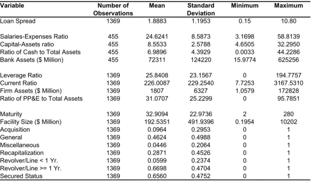
Our empirical analysis uses a sample of1,369U.S. loan facilities between 146banks and1,007
firms from 1996 to 2003. Wefind that positive assortative matching of sizes is prevalent in the loan market, that is, large banks tend to match with largefirms, and vice versa. We then show that for agents on both sides of the market there are similar relationships between quality and size, which lead to similar size rankings for both sides and explain the positive assortative matching of sizes. Banks’ risk and firms’ risk are important factors in their quality. The Bayesian estimates of the loan spread equation are markedly different from the OLS estimates, indicating that controlling for the endogenous matching has a strong impact on the estimates.
The remainder of the paper is organized as follows: Section 2 provides the specification of the model, Section 3 presents the empirical method for Bayesian inference, Section 4 describes the data, Section 5 presents and interprets the empirical results, and Section 6 concludes.
2
Model
The first component of our model is a spread equation, in which the loan spread is a function of the bank’s characteristics, the firm’s characteristics, and the non-price characteristics of the loan. A two-sided matching model in the loan market supplements the spread equation to permit non-random matching of banks and firms.
2.1
Spread Equation
We are interested in estimating the following spread equation:
rij =α0+Bi0α1+Fj0α2+Nij0 α3+ ij ≡Uij0 α+ ij, ij ∼N(0, σ2), (3)
where rij is the loan spread if bank ilends to firm j, Bi is a vector of bank i’s characteristics, Fj
Prior studies, such as Hubbard, Kuttner and Palia (2002) and Coleman, Esho and Sharpe (2004), suggest that the bank’s monitoring ability and risk, as well as thefirm’s risk and information costs are important determinants of the loan spread. Those characteristics are not perfectly observed, so we follow the literature and use proxies for them in the spread equation. Because estimation of our model is numerically intensive, we focus on a parsimonious specification to keep estimation feasible.
Bank’s Monitoring Ability. According to the hold-up theory in Rajan (1992) and Diamond and Rajan (2000), a bank that has superior monitoring ability can use its skills to extract higher rents. Moreover, Leland and Pyle (1977), Diamond (1984, 1991) and Allen (1990) show that banks’ monitoring plays an important role infirms’ operation and provides value to them. Therefore, we expect a bank that has higher monitoring ability to charge a higher spread.
A bank’s salaries-expenses ratio, defined as the ratio of salaries and benefits to total operating expenses, is a proxy for its monitoring ability. Coleman, Esho and Sharpe (2004) show that mon-itoring activities are relatively labor-intensive, and that salaries can reflect the staff’s ability and performance in these activities.
Bank’s Risk. A bank’s risk comes from two sources: inadequate capital and low liquidity. Hubbard, Kuttner and Palia (2002) suggest that a low capital-assets ratio reduces the bank’s ability to extract repayment, therefore lowering the recovery rate in default and forcing the bank to charge a higher spread. Furthermore, a bank that has higher liquidity (or lower liquidity risk) is better able to meet the credit or cash needs of its borrowers, so it charges a higher spread.
A bank’s capital-assets ratio is a proxy for its capital adequacy, and its ratio of cash to total assets is a proxy for its liquidity risk. The size of a bank (its total assets) is also a proxy for its risk, since a larger bank is likely to have better diversified assets and lower risk.
Firm’s Risk. Proxies for a firm’s risk include the leverage ratio (total debt/total assets), the current ratio (current assets/current liabilities), and the size of thefirm.
Risk is positively related to the leverage ratio, so a firm that has a higher leverage ratio is charged a higher spread, all else being equal. On the other hand, afirm with a higher current ratio is considered less risky, so it is typically charged a lower spread. Due to the diversification effects of increasingfirm size,firm risk is negatively associated withfirm assets, and a largerfirm can usually get a loan with a lower spread.
Firm’s Information Costs. In general smaller firms pose larger information asymmetries and are associated with higher information costs, because they typically lack well-documented track records. So the size of afirm is also a proxy for information costs.
Another proxy for a firm’s information costs is the ratio of property, plant, and equipment (PP&E) to total assets, which indicates the relative significance of tangible assets in the firm. A
firm with relatively more tangible assets poses smaller information asymmetries. Consequently it can borrow at a lower spread, all else being equal.
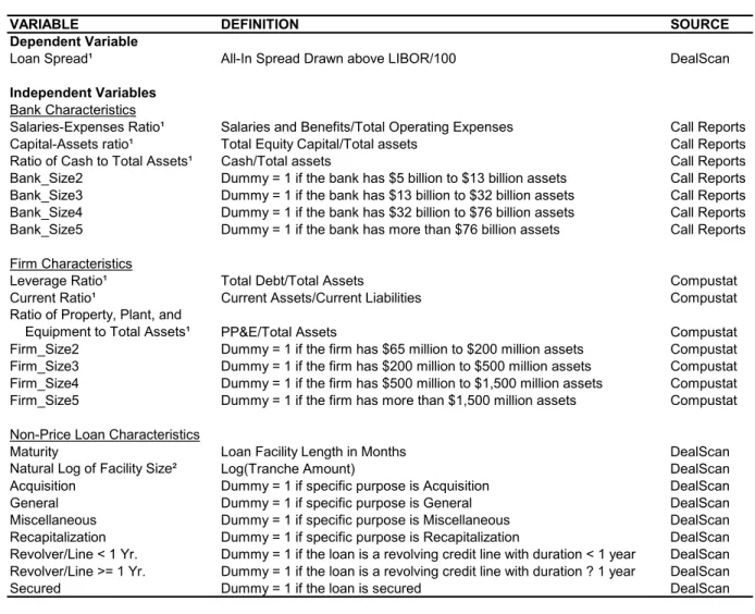
Non-Price Loan Characteristics. Non-price loan characteristics are included on the right-hand side of the spread equation as control variables. They are maturity (in months), natural log of the loan facility size, purpose dummies such as “acquisition” and “recapitalization”, type dummies such as “a revolver credit line with duration shorter than one year”, and a secured dummy. The definitions of these variables are presented in Section 4.
2.2
Two-Sided Matching Model
To take into account the endogenous matching, a two-sided matching model is developed to supple-ment the spread equation and address the sample selection problem resulting from the non-random matching between banks andfirms:
rij = α0+Bi0α1+Fj0α2+Nij0 α3+ ij ≡Uij0 α+ ij, ij ∼N(0, σ2), (4)
Qbi = Bi0β+ηi, ηi∼N(0, σ2η), (5) Qfj = Fj0γ+δj, δj ∼N(0, σ2δ), (6)
mij = I(bank ilends to firmj), (7)
whereQbi is the quality index of banki,Qfj is the quality index of firmj, andI(.) is the indicator function. rij, Nij are observed iff the match indicator mij = 1. ηi and δj are allowed to be
correlated with ij.
In the two-sided matching model, whether mij equals one or zero is determined by both banks’
choices andfirms’ choices, and the outcome corresponds to the unique equilibrium matching (defined later), which depends on theQbi’s and the Qfj’s.
Note that in the loan market, the two-sided matching process between banks and firms takes place before loan spreads are determined. For example, Miller and Bavaria (2003) and Yago and McCarthy (2004) document that in the second half of the 1990’s, “market-flex language” became
common in the loan market, which lets the pricing of a loan be determined after the loan agreement is made. Because of this institutional feature, during the matching process banks andfirms do not know what the loan spreads would be. They take into account the expectation of the spreads, which is a function of the characteristics of the agents. As long as those characteristics are linear in expected spreads, the spread consideration is reflected in the quality indexes and the indexes can be viewed as “spread-adjusted” quality indexes.
Agents, Quotas and Matches. Let It and Jt denote, respectively, the sets of banks and firms in market t, wheret= 1,2, ..., T. It and Jt arefinite and disjoint. The market subscript tis
sometimes dropped to simplify the notation.
In the empirical implementation of our model, a market is specified to contain all thefirms that borrow during a half-year and all the banks that lend to them. In our sample the vast majority of
firms borrow only once during a half-year. In such a short period of time, it is likely that a firm’s
financial needs can be satisfied by a single loan, whereas borrowing multiple loans would increase the administrative costs, such as the costs associated with the negotiation process. Therefore it is reasonable to model that a firm matches with only one bank in a given market.
On the other hand, a bank often lends to multiple firms during a half-year. A bank’s lending activity is restricted in two ways. First, loan assessment, approval, monitoring, and review processes are relatively labor-intensive, and a bank’s lending activity is restricted by the amount of resources that is available for these processes, e.g., the number of its loan officers. Consequently, the number of loans that a bank can make during a given half-year is limited.3 Second, the total amount of loans a bank can make may be constrained by the availability of deposits, the primary source of funds for bank lending (Jayaratne and Morgan, 2000). Jayaratne and Morgan (2000)find evidence that the deposits constraint on bank lending operates only on small banks whose assets are less than $100 million, and that larger banks are unconstrained because they have better access to capital markets. In our sample less than 1% of the banks have assets lower than $100 million, so the lending constraint posed by inadequate deposits is less of a concern. In our study we take the limit on the total amount of loans as non-binding and take the limit on the number of loans as binding to simplify the empirical implementation and make the model tractable.
In market t, bank i can lend to qit firms and firm j can borrow from only one bank. The
model is a special case of the many-to-one two-sided matching model, also known as the College
3
In the long run, the limit on the number of loans that a bank can make during a half-year can change, since the bank can hire or lay offloan officers if needed.
Admissions Model (Gale and Shapley, 1962; Roth and Sotomayor, 1990). qitis known as the quota
of bankiin the matching literature, and everyfirm has a quota of one. We assume that each agent uses up its quota in equilibrium.
The set of all potential loans, or matches, is given byMt=It×Jt. Amatching, μt, is a set of
matches such that (i, j)∈μt if and only if bankiand firmj are matched in market t.
Let μt(i) denote the set offirms that borrow from bank iin market t, and let μt(j) denote the set of banks that lend tofirm j in markett, which is a singleton. We then have
(i, j)∈μt⇐⇒j∈μt(i)⇐⇒i∈μt(j)⇐⇒{i}=μt(j).
Preferences. The matching of banks and firms is determined by the equilibrium outcome of a two-sided matching process. The payofffirm j receives if it borrows from bank i isQbi, and the payoff bank i receives if it lends to the firms in the set μt(i) is Pj∈μ
t(i)Q
f
j. Consequently, each
bank prefers firm j to firm j0 iff Qfj > Qfj0, and each firm prefers bank i to bank i0 iff Qbi > Qbi0. The quality indexes are assumed to be distinct so there are no “ties”.
In our model there is vertical heterogeneity on both sides of the loan market: all banks have identical preference orderings over the firms and all firms have identical preference orderings over the banks. Consequently there is perfect sorting in the market. Vertical heterogeneity is assumed in many economic applications. For example, Wong (2003) assumes that in the marriage market, men and women are ranked by the other side of the market based on their “marriage indexes”. Therefore, all women have a common preference ordering over men, and all men have a common preference ordering over women. Other examples of vertical heterogeneity appear in the market for lawyers in which they are ranked by lawfirms according to their quality (Spurr, 1987), the market for workers in which they are ranked byfirms according to their productivity (Oi, 1983), and so on. Vertical heterogeneity on both sides of the loan market guarantees that the equilibrium matching is unique. We discuss that issue later.
Note that the joint surplus for the pair of bankiand firm j is
sij = Qbi +Q f j
= Bi0β+Fj0γ+ηi+δj
= Bi0β+Fj0γ+ωij.
andδj. As a result,cov(ωij, ωij0)6= 0andcov(ωij, ωi0j)6= 0,∀i6=i0,j6=j0. Therefore the ωij’s are
not independent variables.
Second, in our model the joint surplus depends on bank characteristics andfirm characteristics. A more general model will include pair-specific surplus that depends on pair characteristics, such as the bank’s expertise in the borrower’s industry and the distance between the agents’ headquarters, and the division of the pair-specific surplus between the pair can be endogenous.4 Due to data limitations and tractability concerns, we are unable to include pair characteristics in our model. In the more general model, as long as the magnitudes of the pair-specific surplus are not large enough to change the preference orderings, we will still have vertical heterogeneity on both sides of the market. For example, if the quality indexes are distinct integers and the pair-specific surplus have absolute values smaller than 0.5, then the preference orderings are still determined entirely by the quality indexes.
Equilibrium Matching. A matching is an equilibrium if it is stable, that is, if there is no blocking coalition of agents. A coalition of agents is blocking if they prefer to deviate from the current matching and form new matches among them.
Formally, μt is an equilibrium matching in market t iffthere does not exist I˜⊂It,J˜⊂Jt and
˜
μt6=μt such that ˜μt(i)⊂J˜∪μt(i) and Pj∈˜μ
t(i)Q f j > P j∈μt(i)Q f
j for all i∈I˜, andμ˜t(j)∈I˜and
Qbμ˜ t(j) > Q b μt(j) for all j∈ ˜ J.
The above stability concept is group stability. A related stability concept is pair-wise stability. A matching is pair-wise stable if there is no blocking pair. In the College Admissions Model, Roth and Sotomayor (1990) prove that pair-wise stability is equivalent to group stability and that an equilibrium always exists. Furthermore, Eeckhout (2000, Corollary 3) shows that in a one-to-one two-sided matching model, the equilibrium matching is unique if there is vertical heterogeneity on both sides of the market. Appendix A shows that this sufficient condition for uniqueness also applies to the many-to-one two-sided matching model. Therefore in our model there exists a unique equilibrium matching.
Similar to Sorensen (forthcoming), the unique equilibrium matching here can be characterized by a set of inequalities. These inequalities are constructed based on the fact that there is no blocking bank-firm pair for the equilibrium matching. Consider an arbitrary matching in market
4See Stomper (forthcoming) for a discussion on banks’ industry expertise and Coval and Moskowitz (2001) for a
t,μt. Suppose bankiand firmj are not matched inμt. (i, j)is a blocking pair iffQfj > min
j0∈μ
t(i)
Qfj0 and Qbi > Qbμ
t(j). So (i, j) is not a blocking pair iff Q
f
j < min j0∈μ
t(i)
Qfj0 or Qbi < Qbμt(j). Equivalently,
(i, j) is not a blocking pair iffQfj < Qjif and Qbi < Qbij, where
Qfji = ⎧ ⎪ ⎨ ⎪ ⎩ min j0∈μ t(i) Qfj0 if Qbi > Qbμt(j) ∞ otherwise, and Qbij = ⎧ ⎪ ⎨ ⎪ ⎩ Qb μt(j) if Q f j > min j0∈μt(i) Qfj0 ∞ otherwise.
Now suppose bank iand firm j are matched inμt. Bank iorfirm j is part of a blocking pair iff Qfj < max j0∈f(i)Q f j0 orQbi < max i0∈f(j)Q b
i0, where f(i) is the set of firms that do not currently borrow from bank i but would prefer to do so, and f(j) is the set of banks that do not currently lend to
firm j but would prefer to do so. These two sets contain the feasible deviations of the agents and are given by f(i) = {j∈Jt\μt(i) :Qbi > Qbμt(j)}, and f(j) = {i∈It\μt(j) :Q f j >j0min ∈μt(i)Q f j0}. Therefore, neither bank i norfirm j is part of a blocking pair iff Qfj > Qf
ji and Q b i > Qbij, where Qfji= max j0∈f(i)Q f j0 and Qbij = max i0∈f(j)Q b i0. Let μe
t denote the (unique) equilibrium matching in market t. The above analysis leads to the
following characterization of the equilibrium matching:
μt=μet ⇐⇒ Qbi ∈(Qbi, Qib),∀i∈Itand Qfj ∈(Qfj, Q f j),∀j∈Jt, (8) where Qbi = max j∈μt(i) Qbij, Qbi = min j /∈μt(i) Qbij, Qfj = Qfj,μ t(j), and Qfj = min i /∈μt(j) Qfji.
This characterization of the equilibrium matching is used in the Bayesian inference method in the next section.
3
Estimation
Two-sided matching in the loan market presents numerical challenges when it comes to estimation. Maximum likelihood estimation requires integrating a highly nonlinear function over thousands of dimensions, most of which correspond to the latent quality indexes. Instead we use a Gibbs sam-pling algorithm that performs Markov chain Monte Carlo (MCMC) simulations to obtain Bayesian inference, and augment the observed data with simulated values of the latent data on quality in-dexes so that the augmented data are straightforward to analyze. The method iteratively simulates each block of the parameters and the latent variables conditional on all the others to recover the joint posterior distribution. It transforms a high-dimensional integration problem into a simulation problem and overcomes the computational difficulty.
3.1
Error Terms and Prior Distributions
Estimation of the quality index equations is subject to the usual identification constraints in dis-crete choice models, so ση and σδ are set to one to fix the scales, and the constant and market
characteristics are excluded tofix the levels.
To address the correlation among the error terms, we work with the population regression of
ij on ηi and δj:
ij = κηi+λδj+νij, νij ∼N(0, σ2ν),
cov(ηi, νij) = 0,
cov(δj, νij) = 0.
Thuscov( ij, ηi) =κ,cov( ij, δj) =λ, andσ2 =κ2+λ2+σ2ν. The signs in the two-sided matching
model are identified by requiring λ to be non-positive, consistent with the belief that firms with higher unobserved quality (lower unobserved risk or unobserved information costs) are charged lower loan spreads, everything else being equal.
The prior distributions are multivariate normal forα,β,γ, normal forκ, and truncated normal for λ (truncated on the right at 0). The means of these prior distributions are zeros, and the variance-covariance matrices are 10I, where I is an identity matrix. The prior distribution of 1/σ2ν is gamma, 1/σ2ν ∼G(2.5,1). The above are diffuse priors that include reasonable parameter values well within their supports. We try larger variances and other changes in the priors and the estimates are left almost unchanged. For any parameter, the variance of the prior distribution is at
least 233 times the variance of the posterior distribution, showing that the information contained in the Bayesian inference is substantial.
3.2
Conditional Posterior Distributions
In the model, the exogenous variables areBi,Fj, andNij, which are abbreviated asX. The observed
endogenous variables are rij (the loan spread) and mij (the match indicator). The unobserved
quality indexes areQbi and Qfj. The parameters areα,β,γ,κ,λ, and1/σ2ν, which are abbreviated as θ. In market t, let Xt, rt, μt and Q∗t represent the above variables, where μt embodies all the
mij’s and Q∗t denotes all the quality indexes.
The joint density of the endogenous variables and the quality indexes conditional on the exoge-nous variables and the parameters is as follows:
p(rt, μt, Q∗t |Xt, θ) = I ³ Qbi ∈(Qb i, Q b i),∀i∈It and Qfj ∈(Qfj, Q f j),∀j∈Jt ´ ×Y(i,j) ∈μt φ³rij−Uij0 α−κ(Qbi −B0iβ)−λ(Q f j −Fj0γ); 0, σ2ν ´ ×Yi∈I t φ(Qbi−Bi0β; 0,1)×Y j∈Jt φ(Qfj −Fj0γ; 0,1), (9)
where I(.) is the indicator function and φ(.;μ, σ2) is the N(μ, σ2) pdf. To obtain the likelihood function for market t Lt(θ) = p(rt, μt | Xt, θ), we need to integrate p(rt, μt, Q∗t | Xt, θ) over all
possible values of the quality indexes. Due to endogenous matching in the market, the bounds on each agent’s quality index depend on other agents’ quality indexes, so the integral can not be factored into a product of lower-dimensional integrals. The Gibbs sampling algorithm with data augmentation transforms this high-dimensional integration problem into a simulation problem and makes estimation feasible.
To keep our study tractable, we model the markets as independent, so the product ofp(rt, μt, Q∗t |
Xt, θ) for t = 1,2, ..., T gives the joint density p(r, μ, Q∗ |X, θ) for all the markets. From Bayes’
rule, the density of the posterior distribution ofQ∗ and θconditional on the data is
p(Q∗, θ | X, r, μ) =p(θ)×p(r, μ, Q∗ |X, θ)/p(r, μ|X)
= C×p(θ)×p(r, μ, Q∗ |X, θ) (10)
whereC is a generic proportionality constant andp(θ) is the prior densities of the parameters. Successful application of the Gibbs sampling algorithm requires simple conditional posterior distributions of the quality indexes and the parameters from which random numbers can be
generated at low computational costs. We obtain those distributions by examining the kernels of the conditional posterior densities. For example, if parameter π has density p(π) = C1 ×
exp£−12(π0M π+ 2π0N+C2)
¤
where C1 and C2 are constants, then π ∼ N(−M−1N, M−1). The
conditional posterior distributions are described in Appendix B. They are truncated normal forQbi, Qfj, and λ, multivariate normal for α,β, and γ, normal forκ, and gamma for1/σ2ν.
3.3
Simulation
In the algorithm, the parameters and the quality indexes are partitioned into blocks. Each of the parameter vectors (α, β, γ, κ, λ, and 1/σ2ν) and the quality indexes is a block. In market t the number of quality indexes is equal to the number of agents, |It|+|Jt|, so altogether we have
T
P
t=1
(|It|+|Jt|) + 6 blocks. In each iteration of the algorithm, each block is simulated conditional
on all the others according to the conditional posterior distributions, and the sequence of draws converge in distribution to the joint distribution.5
Bayesian results reported in Section 5 are based on 20,000draws from which the initial 2,000 are discarded to allow for burn-in. Using Matlab 6.5, these iterations took52 hours on a computer running Windows XP with a 1.3 GHZ Intel Pentium M processor. Visual inspection of the draws shows that convergence to the stationary posterior distribution occurs within the burn-in period. Convergence diagnostics from the Geweke test (Geweke, 1992) do not reject the hypotheses of equal means between draws2,001∼3,800(thefirst 10%after burn-in) and draws11,001∼20,000(the last 50% after burn-in). Additionally, the Raftery-Lewis test (Raftery and Lewis, 1992) using all the draws shows that a small amount of burn-in (6draws) and a total of8,700draws are needed for the estimated95%highest posterior density intervals to have actual posterior probabilities between 0.94and 0.96with probability 0.95, indicating that reasonable accuracy can be achieved using the draws we have.
4
Data
We obtain the data from three sources. Information on loans comes from the DealScan database produced by the Loan Pricing Corporation. To obtain information on bank characteristics, we match the banks in DealScan to those in the Reports of Condition and Income (known as the Call Reports) from the Federal Reserve Board. To obtain information onfirm characteristics, we match
5
thefirms in DealScan to those in the Compustat database, a product of Standard & Poor’s.
4.1
Sample
The DealScan database contains detailed information on lending to large businesses in the U.S. dating back to 1988. The majority of the data come from commitment letters and credit agreements in Securities and Exchange Commissionfilings, but data from large loan syndicators and the Loan Pricing Corporation’s own staff of reporters are also collected. For each loan facility, DealScan reports the identities of the borrower and the lender, the pricing information (spread and fees), and the information on non-price loan characteristics, such as maturity, secured status, purpose of the loan, and type of the loan.
We focus on loan facilities between U.S. banks and U.S. firms from 1996 to 2003, and divide them into sixteen markets, each containing all the lending banks and all the borrowing firms in a same half-year: January to June or July to December.6 Data on banks’ andfirms’ characteristics are from the quarter that precedes the market.
A loan facility is included in the sample if the following criteria are satisfied: (1) Data on characteristics of the loan, the bank, and the firm are not missing. (2) If there is more than one lender, one and only one lead arranger is specified.7 (3) The firm borrows only once in the given market. (4) The bank is matched to one and only one bank in the Call Report, and the firm is matched to one and only one firm in the Compustat database.
The sample consists of 1,369loan facilities between 146banks and1,007firms.8 Figure 1 plots the number of banks and the number offirms in each market. The number of banks in each market is relatively stable, while the number of firms exhibits a slightly upward trend. The number of
firms in each market is also the number of loan facilities in each market, since each firm borrows only once in a given market.
6
Changing the market definition from one half-year to one year or one quarter leaves ourfindings largely unaffected.
7When there are multiple lenders, the characteristics of the lead arranger are the most relevant for our analysis
and we take the lead arranger as the lending bank. Angbazo, Mei and Saunders (1998) show that in syndicated loans, the administrative, monitoring, and contract enforcement responsibilities lie primarily with the lead arranger.
8
Some banks and somefirms participated in more than one market. The numbers of banks in the markets add up to455, and the numbers offirms in the markets add up to1,369.
4.2
Variables
Information on loan spreads comes from the All-In Spread Drawn (AIS) reported in the DealScan database. The AIS is expressed as a markup over the London Interbank Offering Rate (LIBOR). It equals the sum of the coupon spread, the annual fee, and any one-time fee divided by the loan maturity. The AIS is given in basis points (1 basis point = 0.01%). Since several exogenous variables in our study are expressed in percentage points, we divide the AIS by100 to obtainrij.
Figure 2 plots the weighted average loan spread in percentage points for each market.
The matching of banks and firms (μ) is given by the names of the matched agents recorded in our loan facilities data.
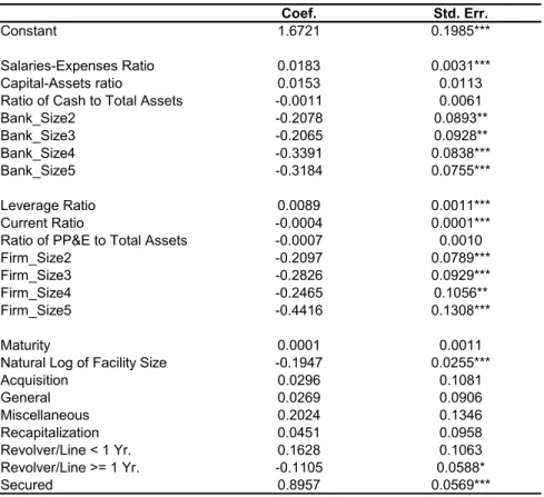
The right-hand side of the spread equation includes a constant, year dummies, and three groups of exogenous variables. Thefirst group includes the following bank characteristics: salaries-expenses ratio (salaries and benefits/total operating expenses), capital-assets ratio (total equity capital/total assets), ratio of cash to total assets (cash/total assets), and four size dummies. Each size dummy corresponds to one fifth of the banks with the cutoffs being $5 billion, $13 billion, $32 billion, and $76 billion in assets. The size dummy for the smallest one fifth is dropped. The size dummies enable us to detect nonlinear relationships between sizes and loan spreads.
The second group includes the following firm characteristics: leverage ratio (total debt/total assets), current ratio (current assets/current liabilities), ratio of property, plant, and equipment (PP&E) to total assets (PP&E/total assets), and four size dummies. Each size dummy corresponds to onefifth of the firms with the cutoffs being $65 million, $200million, $500million, and $1,500 million in assets. The size dummy for the smallest onefifth is dropped.
The third group includes the following non-price loan characteristics: maturity (in months), natural log of facility size, purpose dummies, type dummies, and a secured dummy. The loan purposes reported in DealScan are combined intofive categories: acquisition (acquisition lines and takeover), general (corporate purposes and working capital), miscellaneous (capital expenditure, equipment purchase, IPO relatedfinance, mortgage warehouse, projectfinance, purchase hardware, real estate, securities purchase, spinoff, stock buyback, telecom build-out, and tradefinance), recap-italization (debt repayment/debt consolidation/refinancing and recapitalization), and other. The purpose dummy for “other” is dropped. There are three categories of loan types: revolver/line< 1 year (a revolving credit line whose duration is less than one year), revolver/line ≥ 1 year, and other. The type dummy for “other” is dropped. A secured dummy is also included, which equals
one if the loan facility requires a pledge of assets as collateral, and equals zero otherwise.
The right-hand side variables in the quality index equations are bank characteristics and firm characteristics, respectively. Bank assets, firm assets, and facility size are deflated using the GDP (Chained) Price Index reported in the Historical Tables in the Budget of the United States Gov-ernment for Fiscal Year 2005, with the year 2000 being the base year. All ratios are expressed in percentage points. Table 1 provides the definitions and sources of the variables, and Table 2 presents summary statistics.
5
Findings
In this section, we first present evidence that positive assortative matching of sizes is prevalent in the loan market, that is, large banks tend to match with large firms, and vice versa. We then show that for agents on both sides of the market there are similar relationships between quality and size: after controlling for other factors, the medium-sized agents are regarded as having the highest quality, followed by the largest agents, and the smallest agents are at the bottom of the list. Consequently there are similar size rankings on both sides, which explain the positive assortative matching of sizes. Banks’ risk and firms’ risk are important factors in their quality. The Bayesian estimates of the loan spread equation are markedly different from the OLS estimates, confirming that controlling for the endogenous matching has a strong impact on the estimates. Finally, the effects of bank characteristics, firm characteristics, and non-price loan characteristics on loan spreads are examined.
5.1
Positive Assortative Matching of Sizes
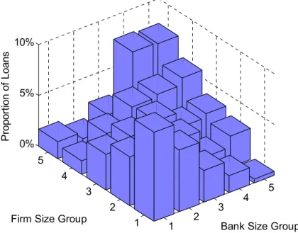
It is recognized in the literature that large banks tend to lend to large firms and vice versa. See, for example, Hubbard, Kuttner and Palia (2002) and Berger et al. (2005). To verify this positive assortative matching of sizes, two OLS regressions using the matched pairs are run: the bank’s size on the firm’s characteristics and the firm’s size on the bank’s characteristics. The results are reported in Tables 3 and 4. It is shown that the bank’s size and thefirm’s size are strongly positively correlated. The coefficients on partners’ sizes are both positive and havet statistics at about 20, indicating that there is indeed positive assortative matching of sizes.
Figure 3 provides further evidence. It depicts the proportion of loans for each combination of bank-firm size groups. For example, the height of the column at (2,3) represents the proportion
of loans between banks in the second bank size group (with assets between the 20th and the 40th percentiles) and firms in the third firm size group (with assets between the 40th and the 60th percentiles). A clear pattern is observed: the highest columns are mostly on the main diagonal (from (1,1) to (5,5)), whereas the columns far off the main diagonal (e.g., (1,5) and (5,1)) are rather short. The figure illustrates that most of the loans are between banks and firms that have similar size positions on their respective sides.
5.2
Quality Indexes
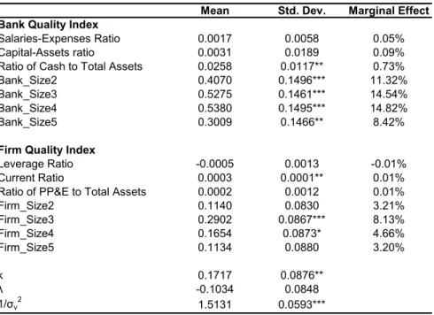
Table 5 reports the posterior means and standard deviations of the coefficients in the quality index equations (5) and (6).
Sizes of the Agents. All the size dummies have positive coefficients and most of them are significant, indicating that on both sides of the market, the group of the smallest agents–the omitted group–is considered the worst in terms of quality.9 On the lenders’ side, the smallest banks suffer from severe lending constraints and low reputation associated with their small sizes. On the borrowers’ side, the smallestfirms are considered the least creditworthy because they have low repaying ability and less diversified assets, and lack well-documented track records to convince the lenders.
A closer look at the coefficients reveals that on both sides of the market, it is the medium-sized agents who have the highest quality. Banks with assets between the 40th and the 80th percentiles (group 3 and group 4) and firms with assets between the 40th and the 60th percentiles (group 3) are the most attractive. The largest agents are less attractive than the medium-sized ones, but are better than the smallest ones.
As the size of a bank increases, it has lower risk and greater lending capacity, making it more attractive. On the other hand, larger banks typically have more severe information distortion problems, and their loan officers have weaker incentives in collecting and processing borrower infor-mation. For the group of the largest banks, these negative effects outweigh the banks’ advantages over the medium-sized banks in terms of risk and lending capacity.
Similarly, as the size of afirm increases, its repaying ability grows, its assets are more diversified, and it can better provide information that is needed to prove its creditworthiness. However, the
9
Here and henceforth statistical significance of Bayesian estimates is taken to mean that zero is not contained in the corresponding highest posterior density intervals.
group of the largest firms are less attractive than the medium-sized firms because lending to the largestfirms means that the bank’s assets will be less diversified and that its control over thefirms’ investment decisions will be weaker, and these disadvantages of the largest firms dominate their advantages over the medium-sized firms.
Note that the negative effect of a firm’s large size on its quality is likely understated, since in our model the limit on the number of loans a bank can make is binding and the limit on the total amount of loans is non-binding. If we take into account that sometimes the binding limit is on the total amount of loans, then lending to a large firm should be less attractive: the size of the loan will typically be large, which means that the bank may have to sacrifice more than one lending opportunity elsewhere in order to lend to this largefirm, impairing the bank’s assets diversification. The size rankings for both sides of the loan market are similar. From the highest quality to the lowest quality, the size ranking is 4-3-2-5-1 for the banks and 3-4-2-5-1 for thefirms, where the numbers represent the size groups. All else being equal, the medium-sized agents have higher quality than the largest ones, which in turn have higher quality than the smallest ones. That explains the positive assortative matching of sizes. Medium-sized banks lend to medium-sized firms because both groups are the top candidates on their respective sides. Among the remaining agents, who face restricted choice sets, the largest banks and the largest firms are the top candidates, so they are matched. Finally, the smallest banks and the smallest firms have the lowest quality, and they have no choice but to match with each other.
Other Factors. On the banks’ side, the coefficient on the ratio of cash to total assets is positive and significant, reflecting the negative impact of banks’ liquidity risk on their quality. The coefficients on the salaries-expenses ratio and the capital-assets ratio are both positive, consistent with the hypothesis that banks with higher monitoring ability and/or higher capital adequacy are more attractive. These two coefficients are insignificant, suggesting that in our sample the influence of these two ratios on the banks’ quality is weak.
On the firms’ side, the current ratio has a positive and significant coefficient, supporting the view that a firm’s quality is negatively related to its risk, for which the current ratio is a proxy. The other two variables both have the expected signs. The coefficient on the leverage ratio is negative, indicating that firms with higher leverage ratios are less attractive because they are riskier. The coefficient on the ratio of PP&E to total assets has a positive sign, suggesting that
asymmetries. The fact that these two coefficients are insignificant indicates that in our sample these two ratios are not important concerns of the banks when they rank the borrowers.
Marginal Effects. For interpretation of the coefficients, Table 5 also reports the marginal effects of the variables. The marginal effect of a variable is defined as the marginal change in an agent’s probability of being preferred to another agent due to a unit difference in the variable. The probability that bank iis preferred to banki0 is
P rob(Bi0β+ηi > Bi00β+ηi0) =P rob(ηi0−ηi < Bi0β−Bi00β) =Φ µ Bi0β−Bi00β √ 2 ¶ ,
whereΦ(.)is the standard normal cdf. The probability thatfirmjis preferred tofirmj0 is obtained analogously. Consider a firm’s choice between two banks. If the two banks have no difference in their observed characteristics, then the choice is completely determined by the unobserved quality, and the probability of each bank being preferred to the other is50%. Now suppose one of the banks is in the smallest group and the other is in the second smallest group, then the probability that the larger bank is preferred to the smaller bank is61.32%, representing a marginal increase of 11.32%. Table 5 shows that banks’ ratios have much larger marginal effects thanfirms’ ratios, and that all the size dummies have noticeable marginal effects. For instance, everything else being equal, a bank in the middle size group is preferred to one in the smallest group with probability 64.54%, and a
firm in the middle size group is preferred to one in the smallest group with probability58.13%.
5.3
Loan Spread Determinants
The covariance between the error terms in the loan spread equation and the bank quality index equation, κ, is found to be significant (Table 5). That is evidence that the matching process is correlated with the loan spread determination and can not be ignored. To see that the mij’s are
correlated with the ij’s, rewrite the spread equation as follows, noting that eachfirm borrows only
once in a market:
rj = α0+m0jBα1+Fj0α2+Nj0α3+ j (11)
= α0+m0jBα1+Fj0α2+Nj0α3+κm0jη+λδj +νj, νj ∼N(0, σ2ν), (12)
whererj is the spread thatfirmjpays,mj = (m1j, m2j, ..., mIj)0 is the vector of match indicators,
B = (B1, B2, ...BI)0 is the matrix of bank characteristics, Nj is the non-price loan characteristics
index equation. Ifmj were in fact independent of j–as it would be iffirms were randomly matched
to banks–then mj would be exogenous in equation (11). However, a significant κ shows that mj
is correlated with j. Because the regressors are correlated with the error term, OLS estimation
of the equation is problematic. Furthermore, since any variable that influences the matching also affects j, the method of instrumental variables (IV) is not applicable here.
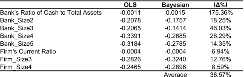
The Bayesian estimates (Table 6) and the OLS estimates (Table 7) of the loan spread equa-tion are markedly different. The average absolute percentage difference, defined as the average of
¯ ¯
¯(ˆθOLS−ˆθBayesian)/ˆθBayesian
¯ ¯
¯ across all the variables including the year dummies, is 23%, where ˆ
θOLS is the OLS estimates andˆθBayesianis the Bayesian estimates. The average absolute percentage
difference for the eight variables that are significant in the quality index equations is39%, signifying the impact of controlling for the endogenous matching on the loan spread equation estimates. Table 8 compares the two sets of estimates side by side for those eight variables. The absolute percentage differences range from 7% to 175%. For instance, the spread differential between a bank in the smallest size group and a bank in the middle size group is overstated by46%when the endogenous matching is ignored.
Directions of the Differences. The unobserved quality of banks has two components that affect the loan spreads in opposite directions: unobserved monitoring ability and unobserved risk. If thefirst component dominates, then the unobserved bank quality will be positively correlated with the loan spreads, because banks with higher unobserved monitoring ability have higher unobserved quality and will charge higher loan spreads, all else being equal. On the other hand, if the second component dominates, then the unobserved bank quality will be negatively correlated with the loan spreads, because banks with lower unobserved risk have higher unobserved quality and will charge lower loan spreads, all else being equal. The positive sign of κ shows that the unobserved monitoring ability dominates the unobserved risk to be the main component in banks’ unobserved quality. The result is an indication that the proxies for banks’ risk do a better job than the proxy for banks’ monitoring ability.
The unobserved quality of firms has two components that affect the loan spreads in the same direction: unobserved risk and unobserved information costs. Firms with either higher unobserved risk or higher unobserved information costs have lower unobserved quality and are charged higher loan spreads, all else being equal. The negative sign ofλis consistent with this relationship.
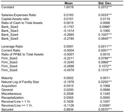
the Bayesian estimates of the loan spread equation are as expected. Five variables have significant coefficients in the bank quality index equation: the ratio of cash to total assets and the four size dummies. All these variables positively affect banks’ quality. Now take the ratio of cash to total assets for example. Suppose all firms are identical except that they have different unobserved quality, and consider two banks that differ only in their ratios of cash to total assets. The bank with a higher ratio has a higher quality, so it matches with a firm that has a higher unobserved quality. Since λ is negative, the higher unobserved quality of the firm means that the spread charged by this bank has a smaller unobserved component. In an OLS regression of the loan spread equation, the effect of that smaller unobserved component on the loan spread is incorrectly attributed to the difference in the ratio, resulting in underestimation (downward bias) of the ratio’s coefficient. Similarly, the coefficients on the four bank size dummies are all underestimated in the OLS regression.
In thefirm quality index equation, three variables have significant coefficients: the current ratio and two size dummies. All these variables positively affectfirms’ quality. Sinceκ is positive, by an analogous argument, the OLS regression of the loan spread equation would result in overestimation (upward bias) of the coefficients on all these variables. That is exactly what happens.
We now analyze the loan spread determinants according to the Bayesian estimates.
Bank Characteristics. The salaries-expenses ratio has a positive and significant coefficient, showing that banks with superior monitoring ability indeed charge higher loan spreads. The
coef-ficients on the capital-assets ratio and the ratio of cash to total assets are insignificant, suggesting that in our sample, banks’ capital adequacy risk and liquidity risk do not have a significant impact on loan spreads. The coefficients on the bank size dummies are all negative and most of them are significant, supporting the view that larger banks are likely to have better diversified assets and hence lower risk, so that they charge lower loan spreads. As expected, these coefficients exhibit a downward trend. Compared to banks with assets below the 20th percentile, banks with assets between the 20th and the 60th percentiles charge loan spreads that are about15basis points lower, whereas banks with assets above the 60th percentile charge loan spreads that are nearly 30 basis points lower.
Firm Characteristics. Two firm ratios have significant coefficients: the leverage ratio (posi-tive) and the current ratio (nega(posi-tive). A higher leverage ratio or a lower current ratio represents a higher borrower risk, so the signs of the coefficients confirm thatfirms with higher risk are charged
higher loan spreads. The coefficient on the ratio of PP&E to total assets is insignificant, suggesting that the ratio does not substantially affect borrowers’ costs of funds. On the other hand, all the
firm size dummies have negative and significant coefficients, consistent with the hypothesis that largerfirms are charged lower loan spreads because they are less risky and are associated with lower information costs. The coefficients on the firm size dummies also exhibit a downward trend. For example, compared to firms with assets below the 20th percentile, firms with assets between the 20th and the 40th percentiles are charged loan spreads that are22basis points lower, whereasfirms with assets above the 80th percentile are charged loan spreads that are 46basis points lower.
Non-Price Loan Characteristics. Three non-price loan characteristics have significant
coef-ficients: the natural log of facility size, the revolver/line>=1 year dummy, and the secured dummy. The negative and significant coefficient on the natural log of facility size is likely due to economies of scale in bank lending. The processes of loan approval, monitoring, and review are relatively labor-intensive, and the labor costs in these processes increase less than proportionally when the size of the loan increases. As a result, a larger loan has a lower average labor costs and is therefore charged a lower loan spread.
The dummy for revolving credit lines whose durations are greater than or equal to one year has a negative coefficient that is significant at the 10% level. Since that type of loans are by far the most common, accounting for67%of all loans, the negative coefficient may reflect that other types of loans are non-standard or even custom-made, and are charged higher loan spreads to compensate for the banks’ extra administrative costs resulting from the loans’ non-standard nature.
The secured dummy has a positive and significant coefficient. An unsecured loan is also called a character loan or a good faith loan, and is granted by the lender on the strength of the borrower’s creditworthiness, rather than a pledge of assets as collateral. The positive coefficient on the secured dummy shows that a higher loan spread is charged if the borrower is below the lender’s threshold for an unsecured loan.
6
Conclusion
We have the potential to learn a lot about financial markets and the effects of monetary policy by investigating the pricing of bank loans. For example, empirical evidence on determinants of loan spreads can provide insights into risk premiums in financial contracting and transmission mechanisms of monetary policy. This paper demonstrates an issue that suggests care in those
efforts. We show that there is endogenous matching in the bank loan market, and that OLS estimation of the loan spread equation is problematic when some characteristics of banks orfirms are not perfectly observed and proxies are used. To control for the endogenous matching, we develop a two-sided matching model to supplement the loan spread equation. We obtain Bayesian inference using a Gibbs sampling algorithm with data augmentation, which transforms a high-dimensional integration problem into a simulation problem and overcomes the computational difficulty.
Using a sample of 1,369 U.S. loan facilities between 146 banks and 1,007 firms from 1996 to 2003, wefind evidence of positive assortative matching of sizes in the market, that is, large banks tend to match with largefirms, and vice versa. We then show that for agents on both sides of the market there are similar relationships between quality and size, which lead to similar size rankings for both sides and explain the positive assortative matching of sizes. Banks’ risk andfirms’ risk are important factors in their quality. The Bayesian estimates of the loan spread equation are markedly different from the OLS estimates, confirming that controlling for the endogenous matching has a strong impact on the estimates. We find that banks with higher monitoring ability charge higher spreads, and larger banks charge lower spreads. On the other hand, firms with higher risk are charged higher spreads, and larger firms are charged lower spreads.
Not only does the two-sided matching model address the endogeneity problem in estimation of the loan spread equation, but it also provides a way to gauge agents’ quality. The latter can be an important feature to include in analyses of various two-sided markets. For instance, in an empirical study of academic achievements or job outcomes of college students (or students in graduate programs, etc.), a two-sided matching model can provide estimates of the colleges’ quality and the students’ ability as useful “by-products”. Other examples include the matchings between teams and athletes (in NBA, for instance), corporations and CEOs,firms and underwriters, and so on. Furthermore, the two-sided matching model enables us to identify the factors that contribute to agents’ quality, which can point the way for agents who try to improve their standing, such as colleges that want to attract better students. This suggests that understanding the quality indexes can play an important competitive role in such markets. We view those issues as interesting avenues for future research.
Appendix A. Uniqueness of Equilibrium Matching
The model described in Section 2 is a special case of the College Admissions Model, for which the existence of an equilibrium matching is proved in Roth and Sotomayor (1990). A new feature of our model is that there is vertical heterogeneity on both sides of the market: all banks have identical preference orderings over thefirms and allfirms have identical preference orderings over the banks. Eeckhout (2000, Corollary 3) shows that in a one-to-one two-sided matching model, the equilibrium matching is unique if there is vertical heterogeneity on both sides of the market. Below we show that this sufficient condition for uniqueness also applies to our many-to-one two-sided matching model.
Re-index the banks and the firms according to the preference orderings, so thatiÂj i0,∀i > i0,
∀j, andjÂi j0,∀j > j0,∀i, whereiÂj i0 denotes that firm j prefers bankito bank i0 and j Âi j0
denotes that bank iprefersfirm j to firmj0. Let qit be the quota of banki. The following J-step algorithm produces the unique equilibrium matching, in which there is perfect sorting. In step 1,
firm J matches with bank I. In step 2, firm J −1 matches with bank I if qIt ≥ 2, otherwise it
matches with bankI−1. In step 3,firmJ−2matches with bankI ifqIt≥3, otherwise it matches
with bank I−1 ifqIt+qI−1,t≥3, otherwise it matches with bankI−2. And so on.
First, μis an equilibrium matching. Suppose not, then there exists at least one blocking pair (i0, j0)such thati0 > μ(j0)andj0>min{j:j ∈μ(i0)}. That is a contradiction, since by construction ifi0> μ(j0) thenj00 > j0,∀j00∈μ(i0), soj0 >min{j:j∈μ(i0)} can not be true.
Second, the equilibrium matching is unique. Suppose not, then there exists μ˜ 6= μ such that ˜
μ is also an equilibrium matching. There is at least one match that is in μ but not in ˜μ. Now consider thefirst step in the algorithm that forms a match that is not in˜μ. Call that match(i0, j0). It follows that min{j : j ∈ ˜μ(i0)} < j0 and that μ˜(j0) < i0, since all the matches formed in the earlier steps are in bothμ andμ˜. Therefore(i0,j0) is a blocking pair for μ˜, a contradiction.
Appendix B. Conditional Posterior Distributions
We obtain the conditional posterior distributions by examining the kernels of the conditional poste-rior densities. The conditional posteposte-rior distribution of Qb
i is N( ˆQbi,σˆ2Qb i
) truncated to the interval (Qbi, Qbi), where ˆ Qbi =Bi0β+κ P j∈μt(i)[rij −U 0 ijα−λ(Q f j −Fj0γ)] σ2 ν+κ2qit , and
ˆ σ2Qb i = σ 2 ν σ2 ν +κ2qit . The conditional posterior distribution of Qfj is N( ˆQfj,σˆ2
Qfj) truncated to the interval(Q f j, Q f j), where ˆ Qfj =Fj0γ+ λ[rμ t(j),j−U 0 μt(j),jα−κ(Q b μt(j)−B 0 μt(j)β)] σ2 ν+λ2 , and ˆ σ2 Qfj = σ2ν σ2 ν +λ2 .
The prior distributions of α, β, γ, andκ are N(¯α, Σ¯α), N(¯β, Σ¯β), N(¯γ, Σ¯γ), and N(¯κ, σ¯2κ),
respectively. The prior distribution of λ is N(¯λ, σ¯2λ) truncated on the right at 0. The prior distribution of 1/σ2ν is gamma, 1/σ2ν ∼G(a, b),a, b >0.
The conditional posterior distribution of αis N(ˆα,Σˆα), where
ˆ Σα = ( ¯ Σ−α1+ T P t=1 P (i,j)∈μt 1 σ2 ν UijUij0 )−1 , and ˆ α=−Σˆα ( −Σ¯−α1α¯− T P t=1 P (i,j)∈μt 1 σ2 ν Uij(rij−κ(Qib−Bi0β)−λ(Q f j −Fj0γ)) ) . The conditional posterior distribution of β isN(ˆβ,Σˆβ), where
ˆ Σβ = ( ¯ Σ−β1+ T P t=1 P i∈It σ2ν+κ2qit σ2 ν BiBi0 )−1 , and ˆ β=−Σˆβ ( −Σ¯−β1β¯+ T P t=1 " P (i,j)∈μt κ σ2 ν Bi(rij−Uij0 α−κQbi −λ(Q f j −Fj0γ))− P i∈It QbiBi #) . The conditional posterior distribution of γ isN(ˆγ,Σˆγ), where
ˆ Σγ= ( ¯ Σ−γ1+ T P t=1 P j∈Jt σ2ν+λ2 σ2 ν FjFj0 )−1 , and ˆ γ=−Σˆγ ( −Σ¯−γ1γ¯+ T P t=1 " P (i,j)∈μt λ σ2 ν Fj(rij −Uij0 α−κ(Qbi−Bi0β)−λQ f j)− P j∈Jt QfjFj #) . The conditional posterior distribution of κ is N(ˆκ,ˆσ2κ), where
ˆ σ2κ = ( 1 ¯ σ2 κ + T P t=1 P i∈It qit(Qbi−Bi0β)2 σ2 ν )−1 , and ˆ κ=−σˆ2κ ( −σ¯¯κ2 κ − T P t=1 P (i,j)∈μt (rij−Uij0 α−λ(Q f j −Fj0γ))(Qbi−Bi0β) σ2 ν ) .
The conditional posterior distribution of λis N(ˆλ,σˆ2λ) truncated on the right at0, where ˆ σ2λ = ( 1 ¯ σ2 λ + T P t=1 P j∈Jt (Qfj −Fj0γ)2 σ2 ν )−1 , and ˆ λ=−σˆ2λ ( − ¯λ ¯ σ2λ − T P t=1 P (i,j)∈μt (rij−Uij0 α−κ(Qbi −Bi0β))(Q f j −Fj0γ) σ2 ν ) . Let n= T P t=1|
Jt|denote the total number of loans in all the markets. The conditional posterior
distribution of 1/σ2ν is G(ˆa,ˆb), where ˆ a=a+n 2, and ˆb= " 1 b + 1 2 T P t=1 P (i,j)∈μt (rij−Uij0 α−κ(Qbi −Bi0β)−λ(Q f j −Fj0γ))2 #−1 .
References
[1] Ackerberg, D. A. and M. Botticini (2002), “Endogenous Matching and the Empirical Deter-minants of Contract Form”,Journal of Political Economy, Vol. 110:3, 564-91.
[2] Albert, J. and S. Chib (1993), “Bayesian Analysis of Binary and Polychotomous Response Data”,Journal of the American Statistical Association, Vol. 88, 669-79.
[3] Allen, F. (1990), “The Market for Information and the Origin of Financial Intermediation”,
Journal of Financial Intermediation, Vol. 1, 3-30.
[4] Angbazo, L., J. Mei and A. Saunders (1998), “Credit Spreads in the Market for Highly Lever-aged Transaction Loans”,Journal of Banking and Finance, Vol. 22, 1249-82.
[5] Berger, A. N., N. H. Miller, M. A. Peterson, R. G. Rajan and J. C. Stein (2005), “Does Function Follow Organizational Form? Evidence from the Lending Practices of Large and Small Banks”,Journal of Financial Economics, Vol. 76:2, 237-69.
[6] Berger, A. N. and G. F. Udell (1990), “Collateral, Loan Quality, and Bank Risk”, Journal of Monetary Economics,Vol. 25, 21-42.
[7] Billet, M., M. Flannery and J. Garfinkel (1995), “The Effect of Lender Identity on a Borrowing Firm’s Equity Return”,Journal of Finance, Vol. 50:2, 699-718.
[8] Brickley, J. A., J. S. Linck and C. W. Smith (2003), “Boundaries of the Firm: Evidence from the Banking Industry”,Journal of Financial Economics, Vol. 70, 351-83.
[9] Coleman, A. D. F., N. Esho, and I. G. Sharpe (2004), “Does Bank Monitoring Influence Loan Contract Terms?” APRA Working Paper No. 2002-01.
[10] Coval, J. and T. Moskowitz (2001), “The Geography of Investment: Informed Trading and Asset Prices”,Journal of Political Economy, Vol. 109:4, 811-41.
[11] Diamond, D. (1984), “Financial Intermediation and Delegated Monitoring”, Review of Eco-nomic Studies, Vol. 51, 393-414.
[12] Diamond, D. (1991), “Monitoring and Reputation: The Choice Between Bank Loans and Directly Placed Debt”,Journal of Political Economy, Vol. 99, 689-721.
[13] Diamond, D. and R. Rajan (2000), “A Theory of Bank Capital”, Journal of Finance, Vol. 55:6, 2431-65.
[14] Eeckhout, J. (2000), “On the Uniqueness of Stable Marriage Matchings”, Economics Letters, Vol. 69, 1-8.
[15] Fernando, C. S., V. A. Gatchev, and P. A. Spindt (2005), “Wanna Dance? How Firms and Underwriters Choose Each Other”,Journal of Finance, Vol. 60:5, 2437-69.
[16] Gale, D. and L. Shapley (1962), “College Admissions and the Stability of Marriage”,American Mathematical Monthly, Vol. 69, 9-15.
[17] Gelfand, A. and A. Smith (1990), “Sampling-Based Approaches to Calculating Marginal Den-sities”,Journal of the American Statistical Association, Vol. 85, 398-409.
[18] Geman, S. and D. Geman (1984), “Stochastic Relaxation, Gibbs Distributions and the Bayesian Restoration of Images”,IEEE Transactions on Pattern Analysis and Machine Intel-ligence, Vol. 6, 721-41.
[19] Geweke, J. (1992), “Evaluating the Accuracy of Sampling-Based Approaches to the Calculation of Posterior Moments” (with discussion), Bayesian Statistics, J. M. Bernardo, J. O. Berger, A. P. Dawid, and A. F. M. Smith (eds.), Vol. 4, 169-93, Oxford University Press.
[20] Geweke, J. (1999), “Using Simulation Methods for Bayesian Econometric Models: Inference, Development and Communication” (with discussion and rejoinder),Econometric Reviews, Vol. 18, 1-126.
[21] Geweke, J., G. Gowrisankaran, and R. Town (2003), “Bayesian Inference for Hospital Quality in a Selection Model”,Econometrica, Vol. 71:4, 1215-39.
[22] Hubbard, R. G., K. N. Kuttner, and D. N. Palia (2002), “Are There Bank Effects in Borrowers’ Costs of Funds? Evidence from a Matched Sample of Borrowers and Banks”, Journal of Business, Vol. 75, 559-81.
[23] James, C. and D. C. Smith (2000), “Are Banks Still Special? New Evidence on Their Role in the Corporate Capital-Raising Process”, Journal of Applied Corporate Finance, Vol. 13:1, 52-63.
[24] Jayaratne, J. and D. P. Morgan (2000), “Capital Market Frictions and Deposit Constraints at Banks”,Journal of Money, Credit, and Banking, Vol. 32:1, 74-92.
[25] Johnson, S. (1997), “The Effects of Bank Reputation on the Value of Bank Loan Agreements”,
Journal of Accounting, Auditing and Finance, Vol. 24, 83-100.
[26] Kashyap, A. K. and J. C. Stein (1994), “Monetary Policy and Bank Lending”, Monetary Policy, N. G. Mankiw (ed.), 221-56, University of Chicago Press.
[27] Lancaster, T. (1997), “Exact Structural Inference in Optimal Job-Search Models”, Journal of Business and Economic Statistics, Vol. 15:2, 165-79.
[28] Leland, H. and D. Pyle (1977), “Informational Asymmetries, Financial Structure and Financial Intermediation”,Journal of Finance, Vol. 32:2, 371-87.
[29] Miller, S. and S. Bavaria (2003), “A Guide to the U.S. Loan Market”, Standard & Poor’s, October.
[30] Oi, W. (1983), “Heterogeneous Firms and the Organization of Production”,Economic Inquiry, Vol. 21, 247-70.
[31] Raftery, A. E. and S. Lewis (1992), “How Many Iterations in the Gibbs Sampler?”Bayesian Statistics, J. M. Bernardo, J. O. Berger, A. P. Dawid, and A. F. M. Smith (eds.), Vol. 4, 763-73, Oxford University Press.