ALGORITHMS FOR STOCHASTIC INTEGER PROGRAMS USING FENCHEL CUTTING PLANES
A Dissertation by
SARAVANAN VENKATACHALAM
Submitted to the Office of Graduate and Professional Studies of Texas A&M University
in partial fulfillment of the requirements for the degree of DOCTOR OF PHILOSOPHY
Chair of Committee, Lewis Ntaimo Committee Members, Sergiy Butenko
Kiavash Kianfar Subodha Kumar Head of Department, C´esar O. Malav´e
August 2014
Major Subject: Industrial Engineering
ABSTRACT
This dissertation develops theory and methodology based on Fenchel cutting planes for solving stochastic integer programs (SIPs) with binary or general integer variables in the second-stage. The methodology is applied to auto-carrier loading problem under uncertainty. The motivation is that many applications can be mod-eled as SIPs, but this class of problems is hard to solve. In this dissertation, the underlying parameter distributions are assumed to be discrete so that the original problem can be formulated as a deterministic equivalent mixed-integer program. The developed methods are evaluated based on computational experiments using both real and randomly generated instances from the literature. We begin with studying a methodology using Fenchel cutting planes for SIPs with binary variables and implement an algorithm to improve runtime performance.
We then introduce the stochastic auto-carrier loading problem where we present a mathematical model for tactical decision making regarding the number and types of auto-carriers needed based on the uncertainty of availability of vehicles. This involves the auto-carrier loading problem for which actual dimensions of the vehicles, regulations on total height of the auto-carriers and maximum weight of the axles, and safety requirements are considered. The problem is modeled as a two-stage SIP, and computational experiments are performed using test instances based on real data.
Next, we develop theory and a methodology for Fenchel cutting planes for mixed-integer programs with special structure. Integer programs have to be solved to generate a Fenchel cutting plane and this poses a challenge. Therefore, we propose a new methodology for constructing a reduced set of integer points so that the generation of Fenchel cutting planes is computationally favorable. We then present the computational results based on randomly generated instances from the literature
and discuss the limitations of the methodology. We finally extend the methodology to SIPs with general integer variables in the second-stage with special structure, and study different normalizations for Fenchel cut generation and report their computa-tional performance.
DEDICATION
ACKNOWLEDGEMENTS
First and foremost, my sincere thanks to my advisor, Dr. Lewis Ntaimo for intro-ducing me to the subject, and for his patience and unconditional support thorough out my research. I would like to thank my committee members, Dr. Sergiy Butenko, Dr. Kiavash Kianfar, and Dr. Subodha Kumar, for their valuable inputs and for introducing me to different facets of academia research. I would also like to thank Dr. Guy L. Curry who inspired me during my graduate days to pursue a career in the field of operations research. I would like to thank the department for their continued support. I am indebted and eternally grateful to my parents, my in-laws and my brother for their patience and support throughout my period of education.
NOMENCLATURE
ALC Auto-Carrier logistic company BAB Branch-and-bound
BAC Branch-and-cut
CPU Central processing unit
DEP Deterministic equivalent problem EV Expected value
FCG Fenchel cut generation FD Fenchel decomposition IP Integer programming ISG Integer set generation LP Linear programming
max Maximum value for the given parameters Max Maximize the objective function
min Minimum value for the given parameters Min Minimize the objective function
MIP Mixed-integer programming MP Master problem
SACP Stochastic auto-carrier problem SFP Starting feasible point
SIP Stochastic integer programming
SMIP Stochastic mixed-integer programming SP Sub problem
ST-FD Stage-wise Fenchel decomposition VSS Value of stochastic solution
TABLE OF CONTENTS Page ABSTRACT . . . ii DEDICATION . . . iv ACKNOWLEDGEMENTS . . . v NOMENCLATURE . . . vi
TABLE OF CONTENTS . . . vii
LIST OF FIGURES . . . ix
LIST OF TABLES . . . xi
1. INTRODUCTION . . . 1
1.1 Motivation and Problem Statement . . . 1
1.1.1 Stochastic Mixed-Integer Programming . . . 2
1.1.2 Fenchel Cutting Planes . . . 4
1.1.3 Stochastic Auto-Carrier Loading Problem . . . 5
1.2 Research Contributions . . . 7
1.3 Dissertation Organization . . . 9
2. LITERATURE REVIEW . . . 10
2.1 Stochastic Mixed-Integer Programming . . . 10
2.2 Fenchel Cutting Planes . . . 14
2.3 Stochastic Auto-Carrier Loading Problem . . . 15
3. FENCHEL DECOMPOSITION FOR STOCHASTIC MIXED 0-1 PRO-GRAMS WITH SPECIAL STRUCTURE . . . 18
3.1 Introduction . . . 18
3.2 Fenchel Decomposition Cut Generation . . . 18
3.3 Stage-Wise Fenchel Decomposition Algorithm . . . 24
3.4 Computational Study . . . 29
3.4.1 Stochastic Multidimensional Knapsack Problems Test Sets . . 29
3.4.2 Computational Results . . . 31
3.4.3 Stochastic Server Location Problem . . . 33
3.4.4 Heuristics for Starting Solution . . . 34
3.5 Conclusion . . . 37
4. STOCHASTIC AUTO-CARRIER LOADING PROBLEM . . . 38
4.1 Introduction . . . 38
4.2 Problem Description . . . 39
4.2.1 Distribution Supply Chain . . . 39
4.2.2 Loading Challenges . . . 41
4.3 Mathematical Formulation . . . 45
4.3.1 First-Stage Formulation . . . 45
4.3.2 Second-Stage Formulation . . . 48
4.4 Solution Scheme and Instance Generation . . . 53
4.5 Computational Study . . . 57
4.6 Conclusion . . . 59
5. FENCHEL DECOMPOSITION FOR MIXED INTEGER PROGRAMS WITH SPECIAL STRUCTURE . . . 60
5.1 Introduction . . . 60
5.2 Fenchel Cut Generation Procedure for General Integer Programs . . . 60
5.2.1 Integer Set Generation for Fenchel Cut Generation . . . 62
5.2.2 Integer Set Generation Algorithm . . . 67
5.2.3 Numerical Example . . . 73
5.3 Computational Study . . . 76
5.3.1 Integer Programs Test Set . . . 76
5.3.2 MIPLIB Instances . . . 79
5.4 Extension to Stochastic Integer Programs . . . 81
5.4.1 Multidimensional Knapsack Instances for SIP . . . 81
5.4.2 Larger Test Instances - I . . . 83
5.4.3 Larger Test Instances - II . . . 88
5.4.4 L1 vs L2 Normalization . . . . 90
5.5 Conclusion . . . 94
6. CONCLUSIONS AND FUTURE WORK . . . 95
6.1 Summary . . . 95
6.2 Future Work . . . 96
REFERENCES . . . 98
LIST OF FIGURES
FIGURE Page
1.1 An auto-carrier with nine loading ramps . . . 6
3.1 Separation problem for binary variables . . . 21
3.2 Percent gap of each test instance . . . 34
4.1 Information and vehicle flow in an auto-carrier supply chain . . . 39
4.2 Process flow for an ALC . . . 40
4.3 Illustration of length advantage (L0-L) due to angular ramps . . . 42
4.4 Auto-carrier showing height advantage due to backward slide on the ramps. . . 43
4.5 A sample case of split ramp . . . 43
4.6 Illustration of load variations at various axles due to angular ramps and vehicle positions . . . 44
4.7 Illustration of instance generation based on action plans . . . 55
4.8 Scenario generation . . . 56
5.1 Separation problem . . . 61
5.2 Separation problem with reduced integer feasible set . . . 62
5.3 Illustration of ISG procedure . . . 71
5.4 ISG procedure - step (d) . . . 74
5.5 ISG procedure - step (e) . . . 76
5.6 Gap percentage for Set1.10 and Set2.10 . . . 85
5.7 Gap percentage for Set3.10 and Set4.10 . . . 85
5.8 Gap percentage for test Set5.10 . . . 86
5.10 Gap percentage for Set1.30, Set2.30, and Set3.30 . . . 89
5.11 Improvement for MIPs solve using ST-FD-R (Set1.30, Set2.30, Set3.30) 89 5.12 Number of Fenchel cuts for Set1.30, Set2.30, and Set3.30 . . . 90
5.13 Gap percentage for Set4.30 and Set5.30 . . . 91
5.14 Number of Fenchel cuts for Set4.30 and Set5.30 . . . 91
LIST OF TABLES
TABLE Page
1.1 Sample vehicle types dimensions (HB- Hatchback) . . . 7
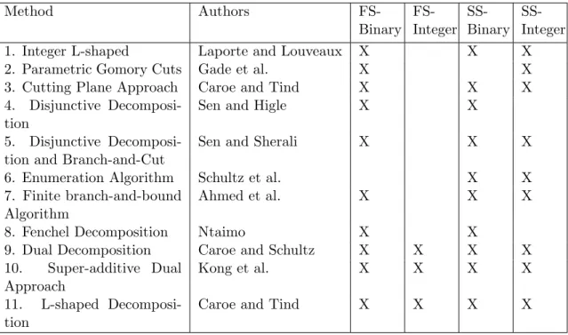
2.1 Literature review . . . 13
3.1 DEP instance characteristics . . . 32
3.2 SSLP instance characteristics . . . 35
3.3 Performance results for larger SSLP instances . . . 37
4.1 Instance characteristics . . . 58
4.2 Runtime characteristics (2 hours) . . . 58
5.1 Instance characteristics - small . . . 77
5.2 Runtime characteristics - small (100 instances for each set) . . . 77
5.3 Instance characteristics - large . . . 78
5.4 Runtime characteristics - large (100 instances for each set) . . . 78
5.5 Problem characteristics - MIPLIB . . . 79
5.6 Runtime characteristics - FCG-ISG . . . 80
5.7 Runtime characteristics - FCG . . . 81
5.8 DEP instance characteristics . . . 84
5.9 Performance characteristics . . . 88
5.10 DEP instance characteristics . . . 88
5.11 Performance characteristics - usingL1 norm . . . . 93
5.12 Performance characteristics - usingL2 norm . . . . 94
A.1 Set 1 Computational results . . . 111
A.3 Set 3 Computational results . . . 113
A.4 Set 4 Computational results . . . 114
A.5 Computational results SSLP instance - I . . . 115
A.6 Computational results SSLP instance - II . . . 116
A.7 Set10.20 Computational results (using L1 norm) . . . 117
A.8 Set30.40 Computational results (using L1 norm) . . . 118
1. INTRODUCTION
1.1 Motivation and Problem Statement
Uncertainty is a key ingredient in many decision making problems. Financial planning, airline scheduling, unit commitment in power systems, and supply chain network planning are a few examples of areas in which ignoring uncertainty of-ten results in sub-optimal decisions. Recent advancements in the availability of computing power and mathematical techniques have made decision making under uncertainty an important field of study. In this research, we study stochastic integer programs (SIPs). SIPs are a class of optimization problems in which some of the input parameters for the model are not known with certainty. We make the assumption that we know the probability distribution of the ‘uncertain’ parameters, and hence the objective function will explicitly include all the outcomes of the uncertain parameter rather than using an expected value for the uncertain parameters. In a two-stage SIP, first-stage decisions are made here-and-now before the future outcomes are known. In the second-stage, the outcomes of the uncertain parameters are considered, and if necessary, corrective or recourse actions are made. The uncertainties in the SIPs are represented by probability distributions.
In the last two decades, there has been a steady growth in the development of efficient solution methods for SIPs. Though there is a considerable amount of literature on solving stochastic programming models with continuous variables in the second-stage, the developments for general integer variables are very limited. This is due to the fact that SIPs are difficult to solve in general. This research develops a new methodology for solving stochastic programs with general integer variables.
1.1.1 Stochastic Mixed-Integer Programming
Following is a two-stage SIP formulation where we minimize the sum of first-stage costs and expected second-stage costs:
SIP2: Min c>x+QE(x) s.t. Ax≥b
x∈X.
(1.1)
In the above formulation, QE(x) denotes the expected second-stage cost based on the first-stage decision x. The setX imposes binary restrictions on all or some com-ponents of x. The objective function coefficients, technology matrix and righthand side are assumed to be stochastic. Therefore, the function QE(x) is given as
QE(x) = EωΦ(q(ω), h(ω)−T(ω)x, ω). (1.2)
The second-stage value function Φ is given as
Φ(ρ, τ, ω) = Min{ρ>y(ω) :W y(ω)≤τ,0≤y(ω)≤u, y(ω)∈Y}. (1.3)
In problem SIP2, x denotes the first-stage decision vector, c ∈ Rn1 is the
first-stage cost vector, b ∈ Rm1 is the first-stage righthand side, and A ∈
Rm1×n1 is the
first-stage constraint matrix. In the second-stage formulation (1.3), y(ω) denotes the recourse decision vector, q(ω) ∈ Rn2 is the cost vector, h(ω) ∈
Rm2 is the
righthand side, T(ω) ∈ Rm2×n1 is the technology matrix, and W ∈
fixed recourse matrix. We also assume thatT(ω) : Ω 7→Rm2×n1,h(ω) : Ω7→
Rm2 and
q(ω) : Ω 7→ Rn2 are measurable mappings defined on a probability space (Ω,F, P).
The function QE(x) is the expected recourse function, where ω is a realization of a multivariate random variable ˜ω, and Eω denotes the mathematical expectation operator satisfyingEω[|Φ(q(ω), h(ω)−T(ω)x), ω|]<∞for allx∈ {Ax≥b, x∈X}. This requirement is the relatively recourse assumption. The set Y is the restriction for the second-stage variables. Finally, the vector u∈ Zn2 defines the upper bound
for the second-stage variables. Subproblem (1.3) is generally referred as the scenario
problem.
A scenario ω will have a corresponding probability pω, and Pω∈Ωpω = 1. If the underlying probability distribution of ˜ωis discrete with a finite number of realizations (scenarios), then the formulation (1.1) - (1.3) can also be written in extensive form, also known as deterministic equivalent problem (DEP) as follows:
DEP : Min c>x+X ω∈Ω pωq(ω)>y(ω) s.t. Ax≥b T(ω)x+W y(ω)≤h(ω) x∈X, y(ω)∈Y. (1.4)
In formulation (1.4), y(ω) is the recourse decision variable vector, and the other dimensions are as stated before.
Even for a reasonable number of scenarios in Ω, DEP is a large scale MIP. With integer variables in both first and second stages, a moderate sized DEP is difficult to solve using a direct solver like CPLEX [40]. This makes a decomposition approach a necessity for most practical sized problems. In SIP2, the type of decision vari-ables (continuous, binary, integer) and in which stage they appear greatly influences
algorithm design. The complexity of the solution methodologies depends on the definitions of the sets X and Y. When X ∈R+ and Y ∈
R+ for a given ω ∈Ω, the
recourse function Φ(ρ, τ, ω) is a well-behaved piecewise linear and convex function of x. Thus, Benders’ decomposition [16] is applicable in this case [108] and the L-shaped method [104] can be used to solve the problems. Assuming fixed recourse (i.e, the recourse matrixW is independent of the scenarioω), the value function of Φ(ρ, τ, ω) will be a piecewise linear function in x. Hence, the L-shaped method works by approximating the linear functions from the subproblems by constructing optimality cuts in the first-stage based on the dual values from the subproblems. However, whenX ∈Z+ andY ∈
Z+, the linear approximation procedure by L-shaped method
is not viable, as the value function is discontinuous, and more precisely the function is lower semicontinuous [19]. Also, the function is non-convex and sub-additive [87]. General efficient methods like the L-shaped method or Dantzig-Wolfe decompo-sition methods are not applicable to SIP. With the integrality restrictions on the second-stage decision variables, dual values from the second-stage program cannot be used to approximate the value function of the second-stage program. Hence, new algorithms or extensions of the L-shaped method are required to handle integer variables in the second or in both of the stages.
1.1.2 Fenchel Cutting Planes
Within a generic framework like L-shaped method, the approach to solve a SIP will be to approximate the value function of the subproblems by solving them as relaxed linear programs (LPs). Based on the dual solution of the relaxed sub-problems, the optimality cuts will be constructed to approximate the second-stage value function. However, in the event of second-stage problems giving non-integer solutions, suitable separation problems are constructed to remove the non-integer solution from further iterations. Construction of valid inequalities via solving
sep-aration problems is an important aspect of this research, where we try to exploit the special structure of the subproblem. In this research, Fenchel cuts will be used as valid inequalities in the second-stage relaxed subproblems. Under certain normalizations, Fenchel cuts are the deeper cuts which guarantee to give facets for the polyhedron. However, for getting the Fenchel cuts, the cut generation procedure involves solving the subproblem as an integer program (IP). In the current literature, Fenchel cuts are used only for subproblems with binary variables. In this research, theory and methodology are devised to generate Fenchel cuts for subproblems with general integer variables.
1.1.3 Stochastic Auto-Carrier Loading Problem
The last mile delivery of cars, trucks and vans to dealerships is one of the most expensive logistics part of vehicle distribution. The final leg of the delivery of vehicles to the dealer lot is invariably carried out by a special type of trucks called auto-carriers. These carriers are specialized trucks with a tractor and a trailer, with upper and lower loading ramps (platforms) as shown in Figure 1.1. An auto-carrier can have anywhere between one and four ramps in each loading level, and a typical version used in delivery of new vehicles has about nine loading ramps. Although vehicle delivery is a specialized transportation problem, this is a very important part of the trucking industry. In 2013 alone, 15.6 million new vehicles were sold in the US [57]. A conservative estimate of $100 per vehicle for the last mile delivery (in general the average cost for the final leg is between $250 and $400) puts the expected expenditure in auto transportation in excess of $15 billion in 2013. The American Trucking Association accords this industry with a special status in their group called Automotive Carrier Conference (ACC).
Figure 1.1: An auto-carrier with nine loading ramps
The auto-manufacturers ship their finished vehicle to a distribution center (DC) through ships and by train. From the staging areas in a DC, the vehicles are shipped to auto dealerships through auto-carriers. Typically a DC receives about 20,000 to 40,000 vehicles a month, and they schedule the delivery to the auto dealerships on a weekly basis. The main objective of a logistics company operating a DC is to reduce the number of trips they make each week to deliver the vehicles. Each trip is subject to loading constraints such as height, length and shape of the vehicle, and also restrictions on maximum length, height and weight of cargo set by local and government organizations such as the U.S. Department of Transportation. Every year, new vehicle types with various dimensions and weights are introduced and this complicates the already difficult loading problem. Table 1.1 shows the wide range of vehicle types, and their dimensions sold by some of the auto-manufacturers in the US. As seen in the table, the heaviest vehicle type is at least three times as heavy as the lightest one, and it requires two loading ramps to transport it. The large quantities of new vehicles being sold each year, the rising cost of fuel, and increasing variety of vehicle types have made this problem very difficult to solve.
Honda Toyota Ford
Ridgeline Accord Fit Tundra Camry Yaris F350 Focus Fiesta Truck Sedan HB Truck Sedan HB Truck Sedan HB Weight (lbs) 6,050 3,216 2,496 6,800 3,190 2,295 9,900 2,097 3,620 Length (inches) 207 195 162 229 189 154 233 179 160 Height (inches) 70 58 60 76 58 59 77 58 58 Width (inches) 78 73 67 80 72 67 80 72 68
Table 1.1: Sample vehicle types dimensions (HB- Hatchback)
Many approaches in current literature use approximation and rule of thumb for auto-carrier loading process. This research presents a tactical planning regarding the number and type of auto-carriers required based on uncertainty in demand for vehicle types. The tactical planning includes an auto-carrier loading problem, which considers actual dimensions of the vehicles, regulations on total height of the auto-carriers, and maximum weight of the axles, and safety requirements. The problem is modeled as a two-stage SIP, and computational experiments using real data are performed.
1.2 Research Contributions
Research contributions include devising of theory and algorithms towards solving SIP2 models based on Fenchel cutting planes. The existing approach of using Fenchel cutting planes for stochastic programs with binary variables exploits the special structure in binary problems. Unfortunately, such direct exploitation is not applicable for SIP with general integer variables. We develop a new algorithm to effectively address the stochastic programs with general integer variables for problems
with special structure. The proposed methodology is tested on randomly generated instances from the literature. The specific research contributions (RC) are as follows:
• RC1: Theory and algorithm for SIP2 with general integer variables in the
second-stage based on Fenchel cutting planes. The methods for generating
Fenchel cutting planes require to solve IPs, which may be difficult in general. Therefore a new algorithm is developed to overcome this challenge.
• RC2: Investigation of normalization for the cut co-efficients in the Fenchel
cutting planes for SIP2. The normalization provides the alignment of the
Fenchel cuts, hence thenorms give the ability for the Fenchel cuts to separate a relaxed solution from the solution space. We investigate the usefulness of different norms, both in terms of computation time and ability to recover integer solutions.
• RC3: Implementation of algorithms from RC1 and RC2. Test the
implemen-tations with randomly generated instances and standard test instances from the literature.
• RC4: Computational study for Fenchel decomposition algorithm SIP2 with
special structure. Perform a computational study based on randomly generated instances from the literature. Also, propose and implement techniques to improve the run time for computational experiments.
• RC5: Formulation for SACP. Generate the instances using real data, and
perform computational experiments using the implementation of the ST-FD algorithm.
future research extensions. The computational study using standard and stochastic auto-carrier instances will provide insights on the practical applicability and limita-tions of the proposed methodology. In a stochastic setup, other general applicalimita-tions with special structure using general integer variables can also benefit directly from using the proposed methodology.
1.3 Dissertation Organization
This dissertation is organized as follows: Literature review for SIP, Fenchel cutting planes, and stochastic auto-carrier loading problem are provided in Section 2. Section 3 details the ST-FD for SIP with binary second-stage recourse problems. Section 4 presents the mathematical model and computational results for SACP. Theory, methodology and computational studies are presented for ST-FD for IP, and SIP with second-stage general integer variables in Section 5. Finally, Section 6 summarizes the contributions of this dissertation, and presents the avenues for future research.
2. LITERATURE REVIEW
This dissertation focuses on using Fenchel cutting planes for SIPs with special structure. This section reviews theory necessary for later sections. It also summa-rizes current state-of-the art approaches for solving SIPs, generating Fenchel cutting planes, and modeling auto-carrier loading problem.
2.1 Stochastic Mixed-Integer Programming
Mathematical programming deals with optimization problems to seek a best solution from the given alternatives. We consider problems with linear constraints and objective function. When all the decision variables of a mathematical program are allowed to take continuous values, and the problem data are known precisely, then the problem is a LP ([42], [33] and [14]). If some or all of the decision variables are restricted to take discrete values then the problem is an IP. Some of the good references for IP are [109], [86] and [71]. A LP with uncertain parameters is a stochastic LP ([41], [58] and [91]). When the data are unknown for the parameters, and some of the variables have integrality restrictions, then it is a SIP. A good introduction to stochastic programming can be found at [18], [58] and [79], and for surveys on SIP, the reader can refer to [65], [98], [59], [94] and [90]. To aid the discussion on the literature, we use a classification scheme to represent the various classes of two-stage SIPs. This scheme is based on the variable restrictions represented by X and Y. We use the sets F and S to denote the first and second stages of the stochastic program, respectively, and B, C, D for binary, continuous and discrete variables, respectively. For example, the class of problems considered in this literature have F ={B, C, D} and S ={B, C, D}, i.e., binary, continuous, and general integer variables may appear in both stages.
The integer L-shaped algorithm [64] is a pioneering methodology for solving SIP. The algorithm solves problems with F = {B};S = {B, C, D}. In the algorithm, the second-stage objective function values are used to construct cuts for the first-stage. However, solving second-stage MIPs to optimality is a challenging task for large scale problems. The work in [27] and [28] uses Lagrangian dual and BAB for F = {B, C, D};S = {B, C, D}. In the algorithm, a non-anticipativity constraint is relaxed, and the corresponding Lagrangian dual is solved to get the Lagrange multipliers. Furthermore, a BAB scheme is used for non-integer solutions. This is a pioneering work to suggest a BAB scheme for solving SIPs. However, the implementation needs very careful devising for choosing appropriate Lagrangian multipliers.
The IP duality in L-shaped framework and Gomory cuts are used in [30] for prob-lems of type F ={B, C, D};S ={B, D}. The subproblems are solved to optimality for a given x ∈ X in a cutting plane algorithm using Gomory cuts. Furthermore, the optimality cuts for master problem are linear functions with integer variables. This is computationally challenging due to the presence of integer variables, and they are required to solve to optimality in the first-stage. In a closely related work [49], a decomposition algorithm for two-stage stochastic programs with binary first-stage and integer second-first-stage variables is proposed. The second-first-stage cost function, technology and recourse matrices are allowed to be random. Since this decomposition method exploits the property that the first-stage variables are binary to derive valid cuts for the second-stage, it is not directly extendable to SIPs with general integer variables in the first-stage.
Cutting plane methods that can partially approximate the second-stage problems within the L-shaped method have been proposed for SIPs with integer variables in the second-stage. In the literature, such methods for two-stage problems have been
almost exclusively restricted to disjunctive cut-generation schemes. In [29], lift-and-project cutting planes approach based on the ideas from [12] is used to solve problems with F = {B, C};S = {B, C}. Cutting planes are used to separate non-integer solutions from the relaxed LPs. In [92], for problems with F = {B};S = {B, C}, disjunctive cuts are developed for the second-stage. Furthermore, the cuts can be made valid across all the other scenarios by calculating an appropriate righthand side function. This has a computational advantage as the cuts need not be generated independently for each scenario. Additionally, the value function is sequentially approximated using linear cutting planes in the first-stage. The work in [95] and [96] uses the framework of reformulation linearization technique. The algorithm in [92] is extended in [93] for problems with S={B, C, D}. A combination of disjunctive pro-gramming and a partial BAB tree is used in the second-stage. Computational studies are reported in [[74] and [75]], [110] for the algorithms of [92] and [93], respectively. Furthermore, the algorithm in [92] is extended in [72] for problems with random recourse and fixed technology matrices. This ensures that the cuts for the second-stage have common coefficients. Another approach using reformulation linearization technique cuts is introduced in [97] for problems with F ={B, C};S ={B, C}.
Method Authors FS-Binary FS-Integer SS-Binary SS-Integer 1. Integer L-shaped Laporte and Louveaux X X X 2. Parametric Gomory Cuts Gade et al. X X 3. Cutting Plane Approach Caroe and Tind X X X 4. Disjunctive
Decomposi-tion
Sen and Higle X X
5. Disjunctive Decomposi-tion and Branch-and-Cut
Sen and Sherali X X X
6. Enumeration Algorithm Schultz et al. X X 7. Finite branch-and-bound
Algorithm
Ahmed et al. X X X
8. Fenchel Decomposition Ntaimo X X
9. Dual Decomposition Caroe and Schultz X X X X 10. Super-additive Dual
Approach
Kong et al. X X X X
11. L-shaped Decomposi-tion
Caroe and Tind X X X X
Table 2.1: Literature review
Continuous variables in the first-stage F = {C} present more difficult prob-lems, as their solutions dictate the orientation of the cutting planes in the second-stage. An enumeration algorithm is developed in [88], and the algorithm is based on polynomial ideal theory (Gr¨obner bases) for problems with F = {C};S = {B, D}. Unfortunately, Gr¨obner bases are notoriously difficult to compute [68]. A finite BAB algorithm is developed in [4] for problems with F = {B, C};S = {B, D} and fixed technology matrix. A formulation to obtain value functions in both the stages is proposed in [62], and problems with F ={B, D};S ={B, D} are studied. Furthermore, a BAB framework in combination with a level-set approach is used as solution methodology. Table 2.1 briefly lists the contributions from the literature.
2.2 Fenchel Cutting Planes
Several types of cutting planes have been proposed in IP. The types of cutting planes include split cuts ([36], [39] and [7]), intersection cuts ([8], [9] and [35]), disjunctive cuts ([11], [12] and [38]) and Fenchel cuts. For a relatively recent review on cutting planes, the reader is referred to [37]. This research work is based on a type of valid inequalities called Fenchel cutting planes. Fenchel cutting planes are a class of deep cutting planes derived using Fenchel duality in convexity theory [81], and they take advantage of the maximum separation/minimum distance duality. Fenchel cuts are suggested in [24], and a number of characteristics are derived in [23], [25] and [26]. The most important results from [24], [25] and [26] are that Fenchel cutting planes are facet defining under certain conditions, and the use of Fenchel cuts in a cutting plane approach yields an algorithm with finite convergence. The work also highlights the fact that generating a Fenchel cut for binary programs is computationally expensive in general; therefore, problems with special structure are desirable to achieve faster convergence. Computational experiments demonstrating the effectiveness of Fenchel cuts are presented for knapsack polyhedra in [22] and for pure binary problems in [25]. Fenchel cuts are derived for two-stage SIPs under a stage-wise decomposition setting in [73]. In [73], consideringx as first-stage decision variable, and y as second-stage decision variable, two forms of cuts called Fenchel decomposition (FD) cuts are derived: one based on the (x, y) space, and the other derived based on the y space, and then lifted ([10] and [13]) to the (x, y) space. However, a direct extension of the current methodology to general integer variables may not be scalable, since solving the subproblems as IPs may be computationally expensive. Also, appropriate normalization should be used in the cut generation process. In this research, we study the effect of different normalizations for the cut-generation procedure.
After the pioneering work in [24], only a few have adopted Fenchel cuts in their work. In [83], Fenchel cuts are used to improve the bounds obtained from MIPs using Lagrangian relaxation. More recently, Fenchel cuts are used to solve deterministic capacitated facility location problems [80]. This work compares Fenchel cuts to Lagrangian cuts in finding good relaxation bounds for their problem. In [20], Fenchel cutting planes are used for findingpmedian nodes in a graph using a cut and branch approach.
2.3 Stochastic Auto-Carrier Loading Problem
To the best of our knowledge this is the first time SIP has been considered in auto-carrier loading problem. In this section, we survey the literature related to auto-carrier loading problem in deterministic setup, and we present on how our approach and features differ from the current literature. Though loading problems are studied in combination with routing, we restrict ourselves to the literature for loading problems. The literature is considered only for the auto-carriers used for loading vehicles for delivery as the loading problems are available in 2-dimensional and 3-dimensional spaces in other areas of applications ([48], [56]). One such example is [55], where the authors have used meta-heuristics for routing with two-dimensional and three-dimensional loading constraints.
The pioneering work on auto-carrier loading problem is presented in [2]. This work is extended in [3]. A quadratic assignment model is presented for auto-carrier loading problem. Vehicle-slot and pairwise incompatibilities are considered for vehi-cles in the adjacent slots. Furthermore, a BAB is presented to solve the quadratic assignment model.
The loading and routing problem is formulated as an IP model in [99]. This work also shows that the problem is NP-hard. Furthermore, a heuristic that considers loading, routing and vehicle selection is proposed. The use of vehicle dimensions
is substituted by a parameter proposed by transportation companies. Based on the parameters from the companies, the total length of the loaded vehicles is constrained. In [69], loading process is simplified so that vehicle dimensions are not considered. The loads are considered in two flat loads with an assumption that any two vehicles can be assigned to the two flat beds. The work proposes a construction heuristics, and presents limited computational results.
A quadratic assignment model very similar to the model suggested in [3] is used in [32]. Furthermore, computational results are presented. The reported results show that the quadratic assignment model produces an exact optimal solution. Similar to the work in [3], compatibility indicators are used for vehicle-slot and pairwise incompatibilities for vehicles in adjacent slots.
An iterated local search approach for both routing and loading of auto-carriers is presented in [44]. Instead of vehicle dimensions, reduction coefficients are used, which are based on auto-carrier type, vehicle type, and slot used for loading. The reduction coefficients are proposed by logistics companies. The reduction coefficients are used to construct restrictions on length of a platform used for loading the vehicles. For each generated route, loading constraints are checked for feasibility. The work also presents extensive computational results.
In all of the works mentioned above, the assignment of vehicles to the slots are constrained based on a parameter value obtained from logistics or transportation companies. These parameters are assumed based on the experience of loaders or loading rules generally maintained in the logistics companies. However, this approach can be cumbersome whenever there are large number of vehicles for loading or vehicles are new to the market. Whenever there are new vehicle types introduced in the market for loading, then generating a reasonable representative parameter for a vehicle is a challenge. Also, in the US we have government regulations on the
maximum weight for each of the axles of an auto-carrier [103]. An approximate estimation for the weight of an auto-carrier’s axle based on the position of vehicle types in the slots is not trivial to estimate. These challenges motivated us to consider the actual dimensions of vehicle types in our mathematical model. Our model considers actual physical dimensions for the vehicle types to estimate the overall length and height, and weight on each axle of the auto-carriers based on the vehicle types loaded in the respective slots.
We presented literature review for SIP and SACP. We reviewed the decomposition approaches available for SIP. SACP is an application of SIP. Hence, a scalable algorithm for SIP will be useful to solve the instances of SACP.
3. FENCHEL DECOMPOSITION FOR STOCHASTIC MIXED 0-1 PROGRAMS WITH SPECIAL STRUCTURE
3.1 Introduction
Decomposition approaches for SIP traditionally fall under one of two categories:
stage-wise decomposition orscenario-wise decomposition. Stage-wise decomposition strategies are usually based on Benders’ decomposition ([16], [104]). Scenario-wise decomposition involves variable splitting on the first-stage decision variables to create nonanticipativity constraints to enforce the first-stage solution to be the same for all scenarios ([28], [82] and [65]). Applications of scenario-wise decomposition can be found in [46], [53], [106] and [70]. In this research, we consider the stage-wise decomposition approach for solving SIP2.
3.2 Fenchel Decomposition Cut Generation
Stage-wise Fenchel decomposition (ST-FD) adopts the Benders’ decomposition setting withxas the first-stage decision variable in the master problem, and yas the second-stage decision variable in the subproblem. In SIP2, instead of working with the IP subproblem directly, ST-FD seeks to find the optimal solution via a cutting plane approach on a partial LP-relaxation of SIP2 where only the subproblems are relaxed. Fenchel cuts are sequentially generated to recover (at least partially) the convex hull of integer points for each scenario subproblem feasible set. If a subproblem LP has a non-integer solution, a Fenchel cut is generated and added to cut off the fractional solution. Fenchel cuts are capable of recovering faces of the convex hull of binary programs, which is the special structure for SIP2. The goal is to construct the convex hull of integer points in the neighborhood of the optimal solution so that by solving subproblems LPs with enough Fenchel cuts added, we
can find the optimal solution without having to use BAB to guarantee optimality. At a given iterationk of the ST-FD cutting plane algorithm, the master problem takes the following form:
zk = Min c>x+θ s.t. Ax≥b
(ηt)>x+θ ≥γt, t∈1, ..., k (3.1a) x∈ {0,1}.
Constraints (3.1a) are theoptimality cuts, which are computed based on the optimal dual solution of all the subproblems. Optimality cuts approximate the value function of the second-stage subproblems. For a first-stage solution xk from the master problem (3.1), the subproblem for each scenario ω ∈ Ω, denoted SP(ω), is given as follows:
SP(ω) : ΦkLP(ρ, τ, ω) = Min ρ>y(ω) s.t. W y(ω)≤τ
βt(ω)>y(ω)≤g(ω, βt(ω)), t∈Θ(ω) (3.2a) y(ω)≥0.
Constraints (3.2a) are the Fenchel cuts, and Θ(ω) is the index set for algorithm iterations at which a Fenchel cut is generated for eachω ∈Ω. Next, we describe how these cuts are generated.
We start with the preliminaries for Fenchel cut generation (FCG) for SIP2. Consider a methodology for FCG to solve problems of type (1.3), especially when
second-stage variables have integer restrictions. We will restrict our discussion to problems of type (1.3) in this section. Also in this section we consider the set Y to have only binary restrictions for some of its components. For ease of exposition, we will ignore the parameter ω in the following derivation. We will start with the definitions.
Let the objective function value of the LP-relaxation to (1.3) be given as,
ΦLP(ρ, τ) = Min{ρ>y:W y≤τ,0≤y≤u, y ∈Rn2}. (3.3)
Feasible set for the problem (3.3) be given as:
FLP ={y:W y≤τ,0≤y≤u, y ∈Rn2}. (3.4)
Let the feasible set for the problem (1.3) be given as:
FIP ={y ∈FLP :y ∈Y}. (3.5)
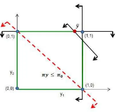
The convex hull of feasible integer points forFIP is represented as C(FIP). Let ˆy∈FLP and ˆy /∈C(FIP) be given. Then the separation problem is to find a valid inequalityβ>y≤β0 for the problem (1.3) such thatβ>y > βˆ 0, where β and β0 are the vectors with appropriate dimensions.
Figure 3.1: Separation problem for binary variables
For illustration, let ˆy ∈ FLP be the optimal solution to the LP-relaxation (3.3) as depicted in Figure 3.1. Using a separation problem, we generate a cut π>y≤ π0 such that π>y > πˆ 0.
In FCG, the objective is to derive such valid inequalities called Fenchel cuts. We start devising the FCG procedure for IPs of type (1.3) with the following theorem. THEOREM 3.1. Let yˆ∈ FLP be given. Define g(β) = Max {β>y | y ∈ C(FIP)}
and let δ(β) = β>yˆ−g(β). Then there exists a vector β for which δ(β)> 0 if and only if y /ˆ∈C(FIP).
Theorem 3.1 is based on generating a Fenchel cut for IPs as proposed in [24], so we omit the proof. The result of Theorem 3.1 is that given a ˆy∈ FLP, if δ(β)>0, then there exists a valid inequality that will separate ˆy from the convex hull of
integer feasible points C(FIP). The inequality derived in such a way is of the form β>y≤g(β) and is called a Fenchel cut. When generating a Fenchel cut, it is desirable to maximize the distance between ˆy and the hyperplaneβ>y≤g(β) without cutting off any integer points in C(FIP). This requires maximizing δ(β).
While any β vector that gives a positive δ(β) will provide a valid Fenchel cut, finding such a β vector requires a search of the β space constrained to a convex set Πβ. Maximizing the function δ(β) provides such a search and returns the deepest cutting plane possible. This maximization provides a Fenchel cut, and separates ˆy from C(FIP). To generate a Fenchel cut, a solution to the following optimization problem is required:
δ = Max β∈Πβ
β>yˆ−g(β) . (3.6)
where the maximization is done over a domain Πβ and
g(β) = Max y∈C(FIP)
β>y . (3.7)
Once found, the Fenchel cut separating the non-integer point ˆy from C(FIP) is:
β>y≤g(β). (3.8)
Note that the cut (3.8) must pass through a point in C(FIP) (found in (3.7)), and could be potentially a facet of C(FIP).
Solving (3.6) is not a trivial task. For this work, a generalized programming method based on Benders’ decomposition is used. The method uses a master problem
(given below) to construct a linear approximation of the subproblem space while the subproblem returns feasible integer points from FIP.
δ(t) = Max β∈Πβ θ
s.t. −θ+ (ˆy−y(ν))>β(ν)≥0, ν = 1,· · · , t.
(3.9)
Let t be the number of iteration, then β(t) represents the value of β in iteration t, and let βi represent a component ofβ. Given an optimal solution (θ(t), β(t)) to (3.9) at iteration t, where y(t) is the optimal solution to the following subproblem:
g(β(t)) = Max β(t)>y s.t. y∈FIP.
(3.10)
It should be noted that solving (3.10) is generally difficult. A straight forward approach will be to solve (3.10) as MIP, however this may not be trivial for larger instances. Adopting a Benders’ decomposition framework, a method for generating Fenchel cuts is stated in Algorithm 1.
In step [1] we initialize the parameters for the algorithm. Initially, each compo-nent ofβ(0) is set to 0.5. Since problem (3.6) has to be solved many times to generate Fenchel cuts, a linearly constrained domain for Πβ such as the L1 unit sphere,
Πβ ={β ∈Rn2+ : 0≤β ≤1,Xβ ≤1}
provides a better choice in terms of solution time. However, an L2 unit sphere,
Πβ ={β ∈R+n2 : 0≤β ≤1,X i
can also be used. Step [2] uses β(0) as co-efficients, then subproblem (3.7) is solved, and the corresponding objective value stored. It should be noted that problem (3.7) is solved as an IP, and this solution y(t) is integral. The bounds and incumbent solutions are updated in step [2]. Based on the solution y(t) from (3.7), the cut is added to master problem (3.9). In step [3], master problem (3.9) is solved and the termination condition is checked. Based on the termination condition, the algorithm either stops or continues.
3.3 Stage-Wise Fenchel Decomposition Algorithm
We extend the algorithm by using L-shaped algorithm to solve the LP-relaxation of SIP2, and then carefully choosing a starting solution for ST-FD algorithm to yield better results. This version of ST-FD algorithm is formally stated in Algorithm 2.
The ST-FD algorithm starts by initializing data in step [1] and getting an initial solution by solving the LP-relaxation of SIP2 in step [2]. If the initial solution satisfies the integrality restrictions for all subproblems in step [3], i.e., x ∈ X and y(ω)∈Y, ∀ω∈Ω, then the solution is optimal, and the algorithm stops. Otherwise, the algorithm continues by calculating and storing the optimality cut coefficients for all subproblems with an integer solution in step [4].
Algorithm 1 Fenchel Cut Generation Procedure (FCG)
[1] Initialization: Set t ← 0, > 0, LB ← −∞, U B ← ∞, and get an initial point β(0)∈Πβ.
[2]Solve subproblem:
Use β(t) to solve (3.7) and get solution y(t) and the corresponding objective value g(β(t)).
Compute lower bound:
Letd(t) ←(ˆy−y(t))>β(t). Setl(t+1)←max{d(t), l(t)}.
if l(t+1) is updatedthen
Update incumbent solution:
Set µ←d(t) and (β∗, g(β∗))←(β(t), g(β(t))).
end if
Use ˆy and solution y(t) from (3.7) to form and add constraint to the problem (3.9). [3] Solve problem (3.9) to get an optimal solution (θ(t), β(t)).
Compute upper bound:
Setu(t+1)←min{θ(t), u(t)}.
if u(t+1)−l(t+1) ≤0 then
The incumbent solution is optimal.
Stop. else
Sett←t+ 1 and go to [2].
Algorithm 2 Stage-Wise Fenchel Decomposition (ST-FD) Algorithm [1]Initialization: setk←0, >0, LB← −∞and U B ← ∞.
[2] Get initial solution: Solve problem (3.1-3.2) using the L-shaped algorithm to get solution (ˆx0,yˆ0(ω)), objective function value ϕ0 = P
ω∈ΩpωΦkLP(ρ, τ, ω), and dual solutions ˆπk(ω) for eachω ∈Ω.
[3]Check solution integrality: if yˆk(ω) ∈Y then
Report (ˆxk,yˆk(ω)) as optimal.
Stop.
end if
[4]Calculate and store optimality cuts coefficients for scenarios with integer solution
forω∈Ωdo
if y(ω)ˆ k ∈Y then
Calculate and store optimality cut coefficientsη(ω)k ← π(ω)ˆ k>T(ω) and γ(ω)k ←
ˆ
π(ω)k>h(ω).
end if end for
[5]Fenchel cuts and optimality cuts generation: forω∈Ωdo
if y(ω)ˆ k ∈/ Y then
Compute scenario Fenchel cut coefficients: Run FCG to getβ(ω)k andg(ω, β(ω)k). Add the cutβ(ω)k>y(ω)≤g(ω, β(ω)k) to subproblem (3.2).
Solve the updated subproblem SP(ω) and get updated subproblem dual solution ˆ
π(ω)k.
Update optimality cut coefficientsηk ←ηk+pω·(ˆπ(ω)k)>T(ω) andγk←γk+pω· (ˆπ(ω)k)>h(ω).
[6]Add optimality cutηkx+θ≥γk to master problem (3.1) and update iterator: set k←k+ 1.
[7]Solve master problem(3.1) to get a new first-stage solution ˆxkand objective value zk.
[8]Update lower bound: SetLB←max{LB, zk}
[9]-optimality check: if |U B−LB| ≤|LB|then Go to step [14]. end if [10]Solve subproblems: forω∈Ωdo
Solve subproblem (3.2) to get updated subproblem solution ˆy(ω)k, optimal value ΦkLP(ρ, τ, ω) and dual solution ˆπ(ω)k.
if y(ω)ˆ k ∈Y then
Calculate and store optimality cut coefficientsη(ω)k ← π(ω)ˆ k>T(ω) and γ(ω)k ←
ˆ
π(ω)k>h(ω).
end if end for
[11]Subproblem solutions integrality check: forω∈Ωdo
if y(ω)k ∈/ Y then
Go to step [5].
end if end for
[12]Update solution and bound information:
Update incumbent solution: x∗ ←xk.
Update upper bound: U B ←min{U B, c>xk+P
ω∈ΩpωΦkLP(ρ, τ, ω)}. [13]-optimality check: if |U B−LB|> |LB|then Go to step [6]. end if [14]Declare x∗ -optimal. Stop.
For subproblems with a solution that does not satisfy the integrality requirements, Fenchel cut coefficients βk(ω), and the righthand side g(ω, βk(ω)) are computed for the iteration k in step [5]. A Fenchel cut is added to subproblem SP(ω). Next, the dual solution obtained by solving the subproblem is used to generate the optimality cut coefficients. Once all subproblems have been solved at a given iteration, the optimality cut is added to the master problem in step [6]. The iteration counter k is increased, and the master problem is solved again in step [7] to get an updated first-stage solution and objective value.
The lower bound LB is updated in step [8]. The gap between the lower bound LB and the upper boundU B is verified in step [9]. If this gap is small enough, then the incumbent solution is declared -optimal in step [14], and then the algorithm terminates. Otherwise, all the subproblems are solved again, and optimality cut coefficients are updated for subproblems with an integer solution in step [10]. The integrality of subproblem solutions is verified in step [11]: if a subproblem’s solution is not integral, the algorithm returns to step [5], to add Fenchel cuts to the subproblems
the incumbent solution x∗ and the upper bound U B are updated in step [12]. The optimality check is done again in step [13]: if it is satisfied, the incumbent solution is -optimal, and the algorithm is terminated. Otherwise, the algorithm returns to step [6], and the optimality cut is added to the master problem, and its solved again. The algorithm is continued until the termination condition is satisfied.
3.4 Computational Study
We implemented the ST-FD algorithm, and performed a computational study to demonstrate the performance of the algorithm on randomly generated instances from the literature. The algorithm was implemented in C++ using CPLEX 12.1 Callable Library [40] in Microsoft Visual Studio 2010. Computations were performed on an ACPI x64 computer with an IntelRXeonRProcessor E5620 (2.4GHz) and 12GB RAM. CPLEX MIP and LP solvers were used to optimize the master problem and subproblems. The instances were run to optimality or stopped when a CPU time limit of 3600 seconds (1 hour) was reached. As a benchmark, the deterministic equivalent problem (DEP) for each test instance was created and solved using the CPLEX MIP solver. Computational experiments were conducted on four sets of test instances from stochastic multidimensional knapsack problems with special structure. Next, we describe the formulation and test sets, and then report computational findings.
3.4.1 Stochastic Multidimensional Knapsack Problems Test Sets
General knapsack constrained stochastic programs have received attention in the literature. Knapsack constraints appear in many applications of SIP such as investment planning ([31] and [54]), transportation, scheduling, selling of assets and investment selection ([60] and [61]) and operations strategy [34]. The stochastic multidimensional knapsack problem test instances we consider were first reported in
a dissertation in [15]. This class of SIP can be formulated as follows: Min n1 X i=1 c>i xi+QE(x) s.t. n1 X i=1 xi ≤b xi ∈ {0,1}, ∀i= 1. . . n1 (3.11)
The functionQE(x) is given as,
QE(x) = EωΨ(ω, x), (3.12)
In problem (3.11), x denotes the first-stage decision vector, c ∈ Rn1 is the
first-stage cost vector, b ∈ R is the first-stage righthand side, Ψ(ω, x) is the recourse function with ωas a realization of a multivariate random variable ˜ω, and Eω denotes the mathematical expectation operator satisfying Eω[|Ψ(ω, x)|] < ∞. The under-lying probability distribution of ˜ω is discrete with a finite number of realizations (scenarios/subproblems) in set Ω and corresponding probabilities pω, ω ∈ Ω. Thus for a given scenario ω ∈ Ω, the recourse function Ψ(ω, x) is given by the following second-stage binary program:
Ψ(ω, x) = Min n2 X i=1 q(ω)i>y(ω)i s.t. n2 X i=1 wijy(ω)i ≤h(ω)j− n1 X i=1 xi, ∀j = 1. . . m2 y(ω)i ∈ {0,1},∀i= 1. . . n2. (3.13)
cost vector, w ∈ Rm2×n2 is the recourse matrix, and h(ω) ∈
Rm2 is the righthand
side.
This formulation has knapsack constraints in both the first- and second-stages, and each subproblem has equal probability of occurrence. Instance data were ran-domly generated using the uniform distribution (U) with different parameter values. The knapsack weights were generated by sampling from U(2,8). Objective function coefficients were generated as done in [105], with the first-stage costs being chosen to be much higher than second-stage costs. Objective function coefficients for first-stage variables were sampled from U(400,650) while those for the second-stage were sampled from U(6,16). To generate tight knapsack constraints, the righthand side value for each of the constraints was generated by finding the maximum knapsack weight (Wmax) for the constraint and sampling from U(2 + 2Wmax,4Wmax).
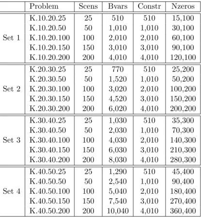
We considered four test sets, each with five randomly generated instances of same size. The problem characteristics are given in Table 3.1. The columns of the table are explained as follows, ‘Problem’ is the instance name, ‘Scens’ is the number of scenarios, ‘Bvars’ is the number of binary variables, ‘Constr’ is the number of constraints, and ‘Nzeros’ is the number of non-zero elements for each of the problem instances. The first numeral in the problem name describes the number of first-stage variables, the second describes the number of second-stage variables, and the third describes the number of scenarios.
3.4.2 Computational Results
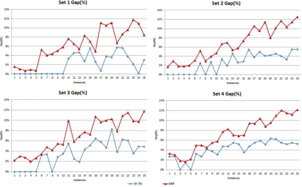
Due to the large number of test instances, we give summary plots of the results to avoid distraction from the discourse and put the detailed numerical results in tables in the Appendix for the interested reader. The computational results in the Appendix are in tables A.1, A.2, A.3 and A.4, with each table reporting results for one of the four test sets. For each instance, five different replications were executed, with an
hour time limit. The columns of the tables are organized as follows: ‘Instance’ is the instance name and the following five columns are based on the runs from ST-FD algorithm. ‘LB’ is the lower bound of the algorithm, and ‘UB’ is the upper bound of the algorithm. ‘FD Cuts’ is the number of Fenchel cuts, ‘%FD’ is the percentage of time taken for generating Fenchel cuts, and ‘%Gap’ is the gap between the LB and UB value after the stipulated runtime of one hour. The final row of each table gives the average of the columns.
Problem Scens Bvars Constr Nzeros K.10.20.25 25 510 510 15,100 K.10.20.50 50 1,010 1,010 30,100 Set 1 K.10.20.100 100 2,010 2,010 60,100 K.10.20.150 150 3,010 3,010 90,100 K.10.20.200 200 4,010 4,010 120,100 K.20.30.25 25 770 510 25,200 K.20.30.50 50 1,520 1,010 50,200 Set 2 K.20.30.100 100 3,020 2,010 100,200 K.20.30.150 150 4,520 3,010 150,200 K.20.30.200 200 6,020 4,010 200,200 K.30.40.25 25 1,030 510 35,300 K.30.40.50 50 2,030 1,010 70,300 Set 3 K.30.40.100 100 4,030 2,010 140,300 K.30.40.150 150 6,030 3,010 210,300 K.30.40.200 200 8,030 4,010 280,300 K.40.50.25 25 1,290 510 45,400 K.40.50.50 50 2,540 1,010 90,400 Set 4 K.40.50.100 100 5,040 2,010 180,400 K.40.50.150 150 7,540 3,010 270,400 K.40.50.200 200 10,040 4,010 360,400
Table 3.1: DEP instance characteristics
Due to the large-scale nature of the instances, an optimality cut suggested in [64] for pure binary first-stage SIP2 was generated and added to the master problem to
completely close the gap between the lower and upper bounds for ST-FD. This was also done in [76] under the D2 algorithms. Finally, the last column is the CPLEX MIP gap after directly solving the DEP for one hour.
The results from the tables are summarized in Figure 3.2 to show the final percent gap at termination of the algorithms. The instances for each test set (five different size instances each with five replications) are numbered 1 to 25 and are plotted on the horizontal axis of each graph. As can be seen from the plots, the results clearly show that ST-FD algorithm gives the best performance compared to DEP. The results show that the ST-FD algorithm scales well with instance size. Notice that as the size of the instances increase (from 1 to 25) so does the percent gap, an indication of increasing problem difficulty. The direct solver generally performs comparatively well on the smaller size instances in each test set, implying that decomposition may not be necessary for such instances.
As can be seen in the tables in the Appendix, most of the computation time in the ST-FD algorithm is spent in generating Fenchel cuts.
3.4.3 Stochastic Server Location Problem
We also tested the ST-FD algorithm on large-scale SSLP instances introduced in [74], and further reported in [76]. These instances were previously solved using disjunctive decomposition (D2) algorithms. Similar to multidimensional knapsack instances, due to the large-scale nature of the SSLP instances, we generated and added the L2 optimality cut [64] to the master problem to close the gap between the lower and upper bounds when x stabilizes. The results show that CPLEX is unable to solve several instances to optimality within the time limit, an indication of problem difficulty. The usage of decomposition methods is therefore necessary.
The characteristics of the instances set used for our computational tests are given in Table 3.2. This set has a total of 45 instances: 9 problem sizes with 5 replications
Figure 3.2: Percent gap of each test instance
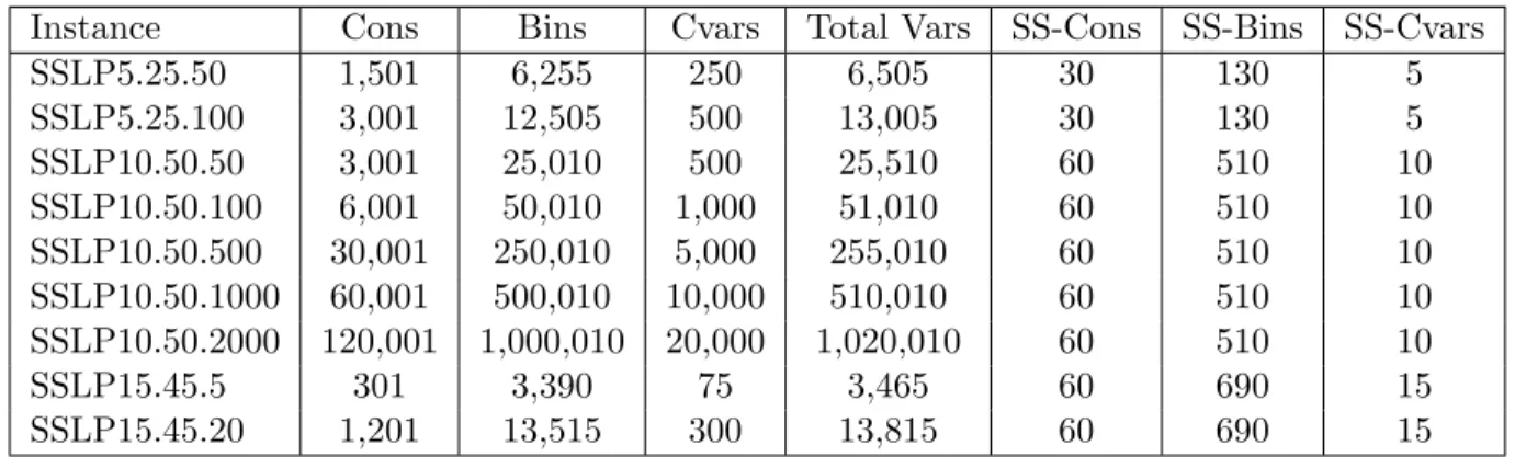
each. The instances are named ‘SSLPm.n.S’, where m is the number of potential server locations, n is the number of potential clients, and S= |Ω| is the number of scenarios. In Table 3.2, ‘Cons’ is the number of constraints for the instance, ‘Bins’ is the number of binary variables, ‘Cvars’ is the number of continuous variables, ‘Total Vars’ is the total number of the variables, ‘SS-Cons’ is the number of second-stage constraints, ‘SS-Bins’ is the number of second-stage binary variables, and ‘SS-Cvars’ is the number of continuous variables in the second-stage.
3.4.4 Heuristics for Starting Solution
Larger SSLP instances needed a significant amount of time to run L-shaped algorithm, where the convergence between the lower and upper bounds was much slower. The purpose of L-shaped algorithm is to provide the ST-FD algorithm with a ‘good’ initial feasible solution. The poor performance of the L-shaped method
Instance Cons Bins Cvars Total Vars SS-Cons SS-Bins SS-Cvars SSLP5.25.50 1,501 6,255 250 6,505 30 130 5 SSLP5.25.100 3,001 12,505 500 13,005 30 130 5 SSLP10.50.50 3,001 25,010 500 25,510 60 510 10 SSLP10.50.100 6,001 50,010 1,000 51,010 60 510 10 SSLP10.50.500 30,001 250,010 5,000 255,010 60 510 10 SSLP10.50.1000 60,001 500,010 10,000 510,010 60 510 10 SSLP10.50.2000 120,001 1,000,010 20,000 1,020,010 60 510 10 SSLP15.45.5 301 3,390 75 3,465 60 690 15 SSLP15.45.20 1,201 13,515 300 13,815 60 690 15
Table 3.2: SSLP instance characteristics
for larger SSLP instances prompted us to devise a Starting Feasible Point (SFP) algorithm. Instead of using L-shaped algorithm in step [2] for ST-FD, we used SFP algorithm. However, with SFP the master problem of the ST-FD algorithm will not have any optimality cuts, since the L-shaped algorithm was not performed. This slows the convergence for ST-FD algorithm. To compensate for the lack of optimality cuts in the master problem, in step [2] of SFP we solved the relaxed subproblems, and provided optimality cuts to the master problem. Finally, in step [3], a lower bound to the master problem was added based on the objective function values from the relaxed subproblems. Finally, in step [4], a constraint is added to master problem (3.1) to set the lower bound for the number of non-zero binary variables based on the solution from solving DEP in step [1]. This criterion is derived based on the knowledge of the problem.
Algorithm 3 Starting Feasible Point Algorithm
[1] Solve the instance as a DEP with binary first-stage variables and continuous second-stage variables to get a binary first-stage solution ˆx and relaxed subproblem solutions ˆy. The runtime is limited to 1800 seconds or a MIP-Gap of 5%.
[2] Solve the relaxed subproblems to get the dual solution using the first-stage solution values, and compute optimality cuts for the master problem.
[3]Bound η in (3.1)using the subproblem objective values. [4] Add a constraint P
ixi ≥m0 to the master problem, where m0 is the number of non-zero solution values from step [1].
3.4.5 Computational Results
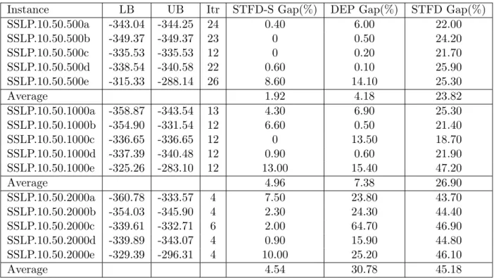
Tables A.5 and A.6 provide the runtime characteristics using ST-FD algorithm for the SSLP instances. Table 3.3 refers the performance results using the improved ST-FD algorithm. The ‘LB’ and ‘UB’ columns refer to the lower and upper bounds obtained using SFP algorithm. The ‘Itr’ column provides the number of iterations performed by the ST-FD algorithm, ‘ST-FD-S Gap (%)’ refers the gap between the lower and upper bound after the stipulated runtime using SFP with ST-FD algorithm, ‘DEP Gap (%)’ is the gap for the DEP solved using CPLEX, and ‘STFD Gap (%)’ is the gap obtained using the standard ST-FD algorithm with the L-shaped algorithm to get the starting feasible solution. The results indicate that SFP algorithm for the starting feasible solution gives better runtime performance as the improvement on the solution gap is below 5% for most of the instances.
Instance LB UB Itr STFD-S Gap(%) DEP Gap(%) STFD Gap(%) SSLP.10.50.500a -343.04 -344.25 24 0.40 6.00 22.00 SSLP.10.50.500b -349.37 -349.37 23 0 0.50 24.20 SSLP.10.50.500c -335.53 -335.53 12 0 0.20 21.70 SSLP.10.50.500d -338.54 -340.58 22 0.60 0.10 25.90 SSLP.10.50.500e -315.33 -288.14 26 8.60 14.10 25.30 Average 1.92 4.18 23.82 SSLP.10.50.1000a -358.87 -343.54 13 4.30 6.90 25.30 SSLP.10.50.1000b -354.90 -331.54 12 6.60 0.50 21.40 SSLP.10.50.1000c -336.65 -336.65 12 0 13.50 18.70 SSLP.10.50.1000d -337.39 -340.48 12 0.90 0.60 21.90 SSLP.10.50.1000e -325.26 -283.10 12 13.00 15.40 47.20 Average 4.96 7.38 26.90 SSLP.10.50.2000a -360.78 -333.57 4 7.50 23.80 43.70 SSLP.10.50.2000b -354.03 -345.90 4 2.30 24.30 44.40 SSLP.10.50.2000c -339.61 -332.71 6 2.00 64.70 46.90 SSLP.10.50.2000d -339.89 -343.07 4 0.90 15.90 44.80 SSLP.10.50.2000e -329.39 -296.31 4 10.00 25.20 46.10 Average 4.54 30.78 45.18
Table 3.3: Performance results for larger SSLP instances
3.5 Conclusion
This section presented the ST-FD algorithm for two-stage SIP2s having special structure with binary variables in the second-stage. The algorithm uses Fenchel cuts generated based on the scenario subproblem under each decomposition setting to iteratively recover (at least partially) the convex hull of integer points in the neighborhood of the optimal solution. In ST-FD, the L-shaped algorithm is the method of choice for solving the LP-relaxation of SIP2 problem. Computational results on knapsack and SSLP instances show that the approach can solve large instances in reasonable amount of time in comparison to a direct solver.
4. STOCHASTIC AUTO-CARRIER LOADING PROBLEM
4.1 Introduction
Auto-carrier loading is the process of assigning vehicles to the ramps of an auto-carrier in an optimal manner. The restrictions in auto-carrier loading include government regulations on the height, weight of the axles, and overall weight of the auto-carrier. An auto-carrier contains ramps for loading the vehicles. Furthermore, the safety of the vehicles is an important factor in the loading process. With these restrictions, an auto-carrier logistic company would like to maximize their revenue by delivering the vehicles, and maintaining a higher load efficiency. In the current literature, most of the approaches focus on the integrated problem of routing and loading ([50], [55] and [45]) of auto-carriers, where the loading problem is looked upon for feasibility for a given optimal route. In our setup, we consider a cluster of loads that are to be delivered to a same destination or zip-code, hence loading becomes an important aspect than routing. Good references for algorithms for vehicle routing include [5], [102], [63] and [51]. We consider the tactical planning for the auto-carrier problem, which deals with deciding the types of resources to be used for actual delivery. Such decisions have to be performed four to five days before the actual delivery of vehicles. Based on the nature of the demand, expected revenue, operating costs of the auto-carriers, and loading challenges, the tactical plan will suggest the required resources for the operations. Using operations decisions for tactical planing has been done in the literature before. This has been done in supply chain context in [84], [47], [89] and [6].
4.2 Problem Description
We start with the details of supply chain of auto-carrier transportation, and then give the details of the loading problem.
4.2.1 Distribution Supply Chain
Auto-manufacturers get requests from the dealers for each of the vehicle types. The dealers’ demands are aggregated at the auto-manufacturer location, and then vehicles are shipped to the auto-carrier locations in large quantities to take advantage of economy of scale. Auto-carriers logistics companies (ALC) receive the vehicles from the auto-manufacturers in bulk quantities, and deliver the vehicles to the dealers based on their demands. Furthermore, the ALCs have processing centers which process the vehicles based on the customization requests from the dealers. The individual customization requests do not provide an economy of scale for the auto-manufacturers. The dealerships need to carry inventory for customization requests, and this will be an operations overload for the dealers. Hence, ALCs are the preferred locations to complete the customization requests.
Figure 4.1: Information and vehicle flow in an auto-carrier supply chain
auto-manufacturers. Based on the production schedule of the auto-manufacturers, the vehicles are transported (typically by rail) to an ALC in mass quantity. In the US, each vehicle is identified by a sixteen digit alpha numeric code named vehicle identification number (VIN). Each VIN is scheduled to be delivered by ALC to a specified dealer. The dealer and ALC co-ordinate for any customization needs for a particular VIN. The processing center at an ALC location processes the individual customer requests, and then the vehicles are transported to the dealers. There are very limited number of ALCs and auto-manufacturers, while the number of dealers is enormous. The core objective of ALC is to distribute the vehicles requested by the dealers at a minimized cost. The revenue for an ALC is based on the type and location of vehicle delivered.
The processes followed at an ALC are depicted in Figure 4.2. The vehicles are delivered at an ALC’s receiving yard from the auto-manufacturers. The vehicles are further processed in the ALC’s processing center, where additional customizations are performed based on individual customer requests. Once the processing of the vehicles is completed, the vehicles are transported by auto-carriers to the dealer locations.
In the US, there are limited ALCs which are delivering vehicles to thousands of dealers. The vehicles vary in size, weight and contour making the loading problem challenging to look at mathematically.
4.2.2 Loading Challenges
ALCs own the auto-carriers used to deliver the vehicles from an ALC’s distribu-tion center to dealers. The number and capabilities of ramps depend on an auto-carrier type. The vehicle can be loaded in two different positions, namely front and back. A front position is where a vehicle faces the front side of an auto-carrier, and the back position is where a vehicle faces the rear side of an auto-carrier. All the ramps can be slid in a forward or backward position. The maximum slide for each ramp is limited, and for modeling purposes, we consider a set of discrete slide angles. The vehicle assignments to the ramps may not be one-to-one as a pair of ramps can hold a single large vehicle. We call this a ‘split ramp’, when more than one ramp is used for holding a vehicle. However, only a specific set of ramps in an auto-carrier can be used as split ramps. Unlike a typical cubing problem, the auto-carrier loading problem is very different with respect to loading flexibility. These flexibilities include sliding the ramps at an angle, changing the vehicle position, and split ramp. For example, vehicles can be loaded at an angle to make adjustments for total height and length of a loaded auto-carrier.
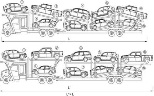
Figure 4.3 shows how the overall length of a loaded auto-carrier changes when some of the ramps are changed from the angular to the flat position. Considering L as the legal length allowed for an auto-carrier, the overall length of auto-carrier L0 exceeds the legal limit when all the upper deck ramps are loaded flat. However, when the same vehicles are loaded in sliding positions, the overall length is within the legally allowed limit.
Figure 4.3: Illustration of length advantage (L0-L) due to angular ramps
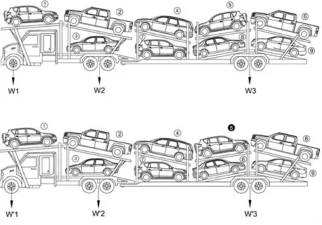
for total height of an auto-carrier. Another example for benefits in height adjustment due to angular ramp adjustment can be seen in Figure 4.4. If the vehicle on ramp 2 is loaded horizontally, it would exceed the legally allowed height limit for the auto-carrier. With the help of an angular ramp, it is possible to get an advantage in height measurement, and satisfy the legal requirement for the loaded auto-carrier. Similarly, a very long vehicle can be loaded in a split ramp. Although this reduces the overall capacity (number of vehicles loaded in an auto-carrier), it helps to load larger vehicles. A sample case of a split ramp is shown in Figure 4.5.
While the above-mentioned flexibility enhances our ability to build