Clustering
Abstract. Network embedding aims at learning the low dimensional representation of nodes. These representations can be widely used for network mining tasks, such as link prediction, anomaly detection, and classification. Recently, a great deal of meaningful research work has been carried out on this emerging network analysis paradigm. The real-world network contains different size clusters because of the edges with different relationship types. These clusters also reflect some features of nodes, which can contribute to the optimization of the feature represen-tation of nodes. However, existing network embedding methods do not distinguish these relationship types. In this paper, we propose an un-supervised network representation learning model that can encode edge relationship information. Firstly, an objective function is defined, which can learn the edge vectors by implicit clustering. Then, a biased random walk is designed to generate a series of node sequences, which are put into Skip-Gram to learn the low dimensional node representations. Extensive experiments are conducted on several network datasets. Compared with the state-of-art baselines, the proposed method is able to achieve favor-able and stfavor-able results in multi-label classification and link prediction tasks.
Keywords: Network embedding·Feature learning ·Edge representa-tion·Network mining.
1
Introduction
Social networks, paper citation networks, gene regulatory networks and oth-er large-scale networks have penetrated into all aspects of our real life. These networks usually have complex structure and large scale. Moreover, the high dimensional and sparse characteristics of networks have brought unprecedent-ed challenges to existing network mining technologies. To solve these problems, network embedding is designed to learn the low dimensional representation of nodes, while preserving the structure and inherent characteristics of the net-work. It can be effectively used by vector-based machine learning models for mining tasks, including node classification, personalized recommendation, and link prediction, etc. [2, 13, 17]
Following the initial ideas in network embedding [17, 22], recent techniques such as DeepWalk [17] and node2vec [13] learn node representation using ran-dom walks sampled in the network. Thereafter, Cao et al. [5] developed a GraRep model, which integrates the global structure information of the network into the learning process. They adopt the idea of matrix decomposition, achieve the di-mensionality reduction by decomposing the relationship matrix, and thus obtain
the network representation of nodes. Tang et al. [19] proposed a large-scale in-formation network embedding method called LINE that preserves both the first-order and second-first-order proximity. Wang et al. [20] designed a Structural Deep Network Embedding (SDNE) model, which maintains the proximity between 2-hop neighbors through deep automatic encoders. Recently, Ribeiro et al. [6] developed a novel and flexible model, called Struc2vec, which uses hierarchical structure to measure the similarity of nodes at different scales, and constructs a multi-layer network to encode the similarity of nodes and generate the structure context for nodes.
However, most of the aforementioned methods mainly focus on the existence of edges between nodes and ignore the differences between edges. A node may be connected with other nodes for different relationship types. The edges with the same relationship types can form a cluster. These clusters hide abundant infor-mation. For example, the similarity between the inner vertices within the same cluster is relatively higher than that within the different clusters. The clusters reflect auxiliary information for network representation learning, and contribute to the generation of more accurate node vectors. In this paper, we propose an unsupervised model for network representation learning, which can strengthen the use of the first-order proximity of network structure and improve accuracy of preserving two-order proximity. Our main contributions can be summarized as follows:
– We propose an unsupervised model for network representation learning, called NEWEE, which can utilize the information of node neighbors as well as the information of the relationship types between nodes.
– We propose a new way to distinguish the relationship types for edges, which can learn similar vectors from similar relationship types without labeling data, and only use the structure information of the network itself.
– Extensive experiments on several datasets demonstrate that our proposed method produces significantly increased performance over the current state-of-the-art network embedding methods in most cases.
The rest of this paper is organized as follows; Section 2, briefly outlines a list of related works and our motivation. Detailed steps of the proposed method are presented in Section 3. Section 4, presents the experiment results, and com-parison with completing algorithms. Finally, this paper is concluded in Section 5.
2
Related Work
Traditional network representation learning methods include network represen-tation learning based on spectral method, such as locally linear embedding (LLE) [18] and laplacian eigenmaps based on manifold assumption [3]. In ad-dition, there is optimization based representation learning for networks, a low-dimensional representation of network can be grasped by optimizing an objec-tive function. Representaobjec-tive algorithms include mapping to homogeneous model
(MTH) [9], content diffusion kernel (CDK) [4], and content-based source diffu-sion kernel (CSDK) [4]. Some scholars improve the description of node content by introducing network information based on subject probability model. Rep-resentative methods include Link-PLSA-LDA [15], relational topic model (RT-M) [23] and probabilistic latent document network embedding (PLANE) [10]. These methods cannot be applied to generalized node feature representation. Besides, most of above-mentioned methods are expensive in calculation and non-expandable for large networks.
Nowadays, representation learning methods are widely applied in the field of natural language processing (NLP), among which, a representative one is word embed-ding [14]. The researchers believe that words with similar contexts should also have similar semantics. The word vectors obtained through unsupervised learning method have achieved excellent performance in many tasks.
Inspired by the above method, the researchers began to apply word embed-ding into feature learning of network nodes [7,8]. Perozzi [17] discovered that the number of words appearing in text corpus and the number of visits for nodes by random walk from network obey exponential distribution. Therefore, Perozzi [17] considered that the Skip-Gram model could be transplanted to representation learning of network as well, and DeepWalk model was propsed [17]. The simi-lar method is Node2vec [1], a process of adjusting random walk by introducing depth first and breadth first strategies based on DeepWalk. Struc2vec [6], an-other type of node embedding strategy, is based on random walk, which finds similar embedding on nodes that are structurally similar. Wang et al. [21] de-veloped an innovative network representation learning framework, called Graph-GAN, which unifiesgenerativemodels and discriminativemodels. The LINE [19] method combined first-order proximity with second-order proximity, which was as the final representation of nodes. The definition of first-order proximity and second-order proximity as follows:
Definition 1(first-order proximity)Given a network G= (E, V), for any two nodes vi and vj. If there is an edge between two nodes, i.e. ei,j ∈ E, Then
there is a first-order proximity between vi and vj.
Definition 2(second-order proximity)Given a network G= (E, V), for any two nodes vi and vj. If there is a common neighbor between two nodes, i.e.
there is a node vk. ei,k ∈ E, ej,k ∈ E, Then there is a second-order proximity
between vi and vj.
Although these methods are fast and effective, all existing methods mainly consider the existence of a link between nodes instead of the difference between these links. Therefore, we propose a new way to distinguish these relationship types, which can encode the edges to update network by implicit clustering, and without labeling data. Then a biased random walk from the updated network can generate more accurate node sequences.
3
The Proposed Model
The problem in this paper is how to construct a suitable model for network representation learning, which can map the networks data to a low-dimensional vector space. Each low-dimensional vector represents one node, and the relation-ships between these vectors reflect the first-order and the second-order proximity between nodes.
3.1 Framework
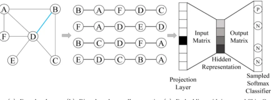
In this section, we describe the main steps of NEWEE model. The flow-graph of the proposed model is shown in Fig. 1. The NEWEE model is divided into three phases, which are described in the following procedure:
1. The edge sampling is used to optimize an objective function, and to learn a low-dimensional representation for each edge in the network. If the relation-ship type of two edges is similar, their vectors are similar as well;
2. By learning the edge vectors from the first phase, a biased random walk is adopted, which can increase the similarity of the two edge vectors before and after walking;
3. The node sequences are obtained from the second phase as the input of Skip-Gram. The original Skip-Gram model only indirectly preserves part of the first-order proximity. Therefore, the improvement of the original Skip-Gram model is made to enhance the similarity between directly connected nodes.
Fig. 1. Overview of NEWEE model: (a) Encode edge: Reconstruct the network and learn a low-dimensional representation for each edge in network. If the relationship type of two edges is similar, their vectors are similar as well; (b) The node sequences generated by biased random walk from the network; (c) Embedding with improved Skip-Gram.
3.2 Encode Edge
The purpose for encoding edges is to learn a low-dimensional representation for each edge of the network. If the relationship types between two edges are similar, their vectors are also similar. We have noticed that a node can be clustered with other nodes due to different relationship types, so the node neighbors can be divided into different neighbor clusters, and the relationship types among different neighbor clusters are different. That means we only need to train one model, which ensures the similarity of the inner edges of the same neighbor clusters, is higher than that of the outer edges of the clusters. Here, we first introduce the concept of self-centered network.
Definition 3(self-centered network)Given a network G = (E, V). For any node vi in G, its self-centered network is G
0
= (E0, V0). The node set V0 includes the node vi and its neighbors, and E
0
represents the set of edges between all nodes in V0.
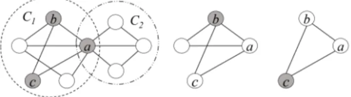
Each node has its own centered network. Fig. 2 (left) shows the self-centered networks of node a. The neighbors of node a are divided into two neighbor clusters of C1 and C2, b and c belong to C1. We have also noticed
that most of the edges in C1 also exist in the self-centered networks of b and
c, as shown in Fig. 2 (middle and right). In general, the closer the cluster is, the more edges exist simultaneously in the self-centered networks of the multiple nodes within the cluster; conversely, if multiple edges exist simultaneously in the self-centered networks of multiple nodes, the multiple edges should belong to the same cluster. Thus, we cannot only avoid explicitly calling clustering algorithm to cluster the node neighbors, but also use the nature of the network itself to implicit clustering.
Fig. 2.The self-centered networks of nodesa (left),b (middle) andc (right). In order to make the similarity of edge vectors of the same self-centered networks higher than that of the other self-centered networks, the objective function is defined as follows:
max X
v∈V0
X
e∈E0
logP(v|e) (1)
WhereP(v|e) is the probability that the network is the self-centered network of nodev when the edge ise. To achieve the purpose of making the edge vectors
of the same self-centered networks similar, we regard it as a binary classification problem, and use the logical regression as the classification method to reconstruct the probability function. The negative sampling technique [16] is used to speed up the training. For∀u ∈V, we first define the following indication function:
Iv(u) =
1, u=v
0, u6=v (2)
For a given nodev, the set of negative sampling isNST(v). The probability function (1) is reconstructed by using negative sampling technique as follows:
P(v|e) =Yu∈{v}∪N STe(v)P(u|e) P(u|e) = σ eTθu , Iv(u) = 1 1−σ eTθu , Iv(u) = 0 (3)
Where σ is the sigmoid function. The parameter θu is the vector of node
u. e is the vector of edge e, and is the final output. It is obtained by bitwise operations of the vectors of two ends of edge. In order to adapt to both the directed networks and the undirected networks, the average operation is used. That is, two ends of edge e are respectively vi and vj. The edge vector ei,j is
denoted as follows:
ei,j=
vi+vj
2 (4)
The final objective function is:
max X v∈V0 X ei,j∈E0 X u∈{v}∪N STei,j(v) L(v, e, u) L(v, e, u) =Iv(u)·log σ eTi,jθu + [1−Iv(u)]·log 1−σ eTi,jθu (5)
We use gradient descent method to optimize the formula (5). First, we con-sider the gradient ofL(v,e,u) onθu.
∂L(v, ei,j, u) ∂θu = ∂ ∂θu Iv(u)·log σ eTi,jθu + [1−Iv(u)]·log 1−σ eTi,jθu
=Iv(u)1−σ eTi,jθuei,j−[1−Iv(u)]σ eTi,jθ u
ei,j
=Iv(u)−σ eTi,jθuei,j
(6) The update formula ofθu is:
θu=θu+η
Iv(u)−σ eTi,jθu
ei,j (7)
Whereη is the learning rate. Then, we consider the gradient ofL(v, e, u) aboutei,j. Becauseei,jandθu are symmetrical inL(v,e,u), it is easy to obtain
∂L(v, ei,j, u)
∂ei,j
=
Iv(u)−σ eTi,jθu
θu (8)
According to the continuous derivation rule and the symmetry ofvi and vj
in ei,j. ∂L(v, ei,j, u) ∂vi =1 2 Iv(u)−σ eTi,jθu θu (9)
The update formula ofvi is:
vi=vi+ η 2 X u∈{v}∪N STei,j(v) Iv(u)−σ eTi,jθu θu (10)
The update formula ofviis same tovj. If inputting the self-centered networks
of multiple nodes, the following situations will occur:
– The similarity between the inner edges within the same self-centered net-work will be higher than that within the different clusters. For example, when inputting the self-centered networks of the nodesa,b,c, and the edges similarity in clustersC1 andC2 will be constantly strengthened;
– The similarity between edges within the different self-centered networks will be weaken. For example, when inputting the self-centered networks of the nodesa, b, c, and the similarity between edges in clustersC1 andC2
con-stantly weaken.
3.3 Learning node features
This section mainly describes how to use the edge vectors obtained in the first phase to train nodes. Like the article [1, 17], which first obtain a series of node sequences by random walk from the network, but we adopt a biased random walk. In particular, by learning the edge vectors from the first stage, the similarity of the two edge before and after walking can be increased, so that the preservation accuracy of the second-order proximity of the network structure can be improved. Then, the node sequences are as the input of Skip-Gram model.
Biased random walk. After the first phase, we get a network with edge vectors, which preserves the relationship types information. Then, a series of node sequences are obtained by a biased random walk from the network. If the started node is v0, the next walk node is randomly selected from its neighbors
asv1. If the current walk node isvk(k ≥1), the selection of the next walk node
vk+1follows the following probability distribution:
P(vk+1=x|vk =v, vk−1=t) =
π(t,v,x)
Z , ev,x∈E
0, otherwise (11)
WhereZ is a normalization constant.π(t,v,x) is a transition probability of walking from nodet to nodev and then walking from nodev to node x:
π(t, v, x) = µ, if x=t similarity(et,v, ev,x), if x6=t and ev,x∈E 0, otherwise (12)
Where µ is a return parameter and set to 0.5. In addition, we use cosine similarity to calculatesimilarity.
similarity(et,v, ev,x) =
et,v·ev,x
ket,vk · kev,xk
(13) Whereet,v and ev,x are the vectors of edgeet,v andev,x respectively. They
are learned from the first phase. Each node in the network is taken as the walk started node of the sequence in turn, and sampling the neighbors1according to
the selection probability distribution of neighbors. For each walk started node v0, we do biased random walk from the network to get a node sequence with
lengthl. After repeating the above operationr times, a series of node sequences are obtained.
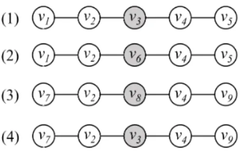
Example. There are two node sequences ofhv1,v2, v3, v4,v5iand hv1, v2,
v6, v4, v5i (Fig. 3). The nodes v3 and v6 have similar contexts, so they can
learn the similar learning representations. In order to get the node sequences of (1) and (2), the edge vector e1,2 should be similar to e2,3, and the edge
vector e2,6 should be similar to e1,2. That is, the edge vector e2,3 should be
similar to e2,6. If adopting the random walk method of DeepWalk, it may get
the node sequences of (2), (3), and (4).v3andv6may have similar left and right
neighborsv2 andv4, but due to the uncertain relationship type, it is difficult to
have the opportunity to reappear bothv1andv5in the nodes extending forward
and backward, which greatly reduce the context similarity ofv3and v6. On the
contrary, if the relationship types between nodes (v3andv8) and their neighbors
(v2andv4) are not similar, the conclusion ofv3similar tov8is not credible even
their contexts are similar.
According to the rule of NEWEE model for generating node sequences, any two connected edges have a high similarity in the sequence. If the two node se-quences are similar, the edges of the two sese-quences are also similar. Conversely, If the nodes have different relationship types with their neighbors. As shown (2) and (3), with the sequence extends the similarity of the learned vector represen-tation ofv6 andv8is decreased.
Improved Skip-Gram. As mentioned above, we have enhanced the utiliza-tion of first-order proximity. The objective funcutiliza-tion of Skip-Gram can achieve similar vectors from nodes with similar contexts. We make the improvement to it as follows: Y ˜ w∈C(w) p(w|w˜)→ Y ei,j∈E p(vi, vj) Y ˜ w∈C(w) p(w|w˜) (14)
Wherep(vi,vj) is used to preserve first-order proximity, and defined as: 1
The alias sampling algorithm [12] method can be used to complete the sampling process in the time complexity ofO(1).
Fig. 3.An example of the influence of relationship type information on the node se-quences (same type lines mean similarity relationship type).
p(vi, vj) =σ viTvj (15)
Whereviandvjare vector representations of nodeviandvjas context nodes
respectively. When the sequences are put into the improved Skip-Gram model, the nodes with similar contexts will be similar.
3.4 Complexity Analysis
In the first phase, the time complexity of training the edge vectors isO(|V|·kndi), where|V|is the number of nodes in the network,kis the average degree of nodes, n is the number of negative sampling,d is the dimension of edge vectors, andi is the number of iterations. The parameters n,d and i are constants. The time complexity of the first phase is linear correlation with the number of nodes|V|. The second phase includes random walk and training a Skip-Gram model. The time complexity of random walk isO(|V|·kdrl), wherer is walk times,l is the length of the node sequence, these parameters are all constants. The time complexity of the random walk is also linear correlation with the number of nodes|V|. As for training a Skip-Gram model, its time complexity isO(swndi), where s is the number of nodes in the input document andw is the size of the context window. The time complexity of training a Skip-Gram model is linear correlation with the number of nodes s. Therefore, the overall computational time complexity of NEWEE isO(|V|·kndi+|V|·kdrl+swndi).
4
Experiments
In this section, we mainly consider the method of quantitative analysis for the NEWEE model. In order to fully describe the effectiveness of our model, the experiments are conducted on the two tasks of link prediction and multi-label classification. For the sake of verifying the robustness and efficiency, the ex-periments are performed from the perspectives of parameters sensitivity and the running time for learning different size networks. Furthermore, we also ap-ply the same networks in the competing algorithms, including DeepWalk [17],
LINE [19], AANE [8], Stru2vec [6], GraphSAGE [7] and Node2Vec [1]. The pa-rameters of the six comparison algorithms are set in such a way that they either take advantage of the default settings suggested by the authors or adjust them experimentally to find the best Settings. After applying these network embed-ding algorithms, the representation of low-dimensional nodes can be obtained respectively.
4.1 Parameter Settings
The default settings of our parameters are mostly consistent with those in article [20]: the negative sampling parameters n1 andn2 are both set to 5. The vector
dimensionsd1andd2are both set to 128. The number of walks started per node
r is 10. Each sequence length l and the size of context window w is set to 80 and 10 respectively.
4.2 Evaluation Metrics
For link prediction, we useprecision@k andMean Average Precision (MAP) to evaluate the performance. Their definitions are listed as follows:
precision@k is a metric, which gives equal weight to the returned instance. It is defined as follows:
P recision@k=| {ei,j|vi, vj∈V, index(ei,j)< k,4i,j= 1} |
k (16)
Where E00 is a hidden edge set hidden in the network. ei,j represents an
edge between nodes vi andvj. index(ei,j) is the ranked index of an edgeei,j in
prediction results.4i,j = 1 indicates an edgeei,j exists inE
00 .
Mean Average Precision (MAP) is a metric with good discrimination and stability. Compared with Precision@k, MAP pays more attention to the instances of ranked ahead in prediction results. It is defined as follows:
AP = P|E 00 | i=1 P recision@i· 4i |E00| , M AP = PQ j=1AP(j) Q (17)
Where4i is an indicator function. When the i-th prediction result is hit, the value4i is 1, otherwise, it is zero.Q is query times.
For multi-label classification, we adoptMacro-F1andMicro-F1as evaluation indexes. Specifically, SupposeC is a label set andAis a label. We denoteTP(A), FP(A) and FN(A) as the number of true positives, false positives and false negatives in the instances which are predicted as A, respectively. F1(A) is the F1-measure for the labelA.Micro-F1 andMacro-F1 are defined as follows:
P r= P A∈CT P(A) P A∈C(T P(A) +F P(A)) , R= P A∈CT P(A) P A∈C(T P(A) +F N(A)) M acro−F1 = P A∈CF1 (A) |C| , M icro−F1 = 2·P r·R P r+R (18)
4.3 Multi-label Classification
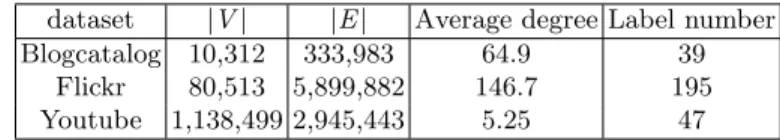
Multi-label classification is an important task to measure the effectiveness of network representation. We select three social networks to perform multi-label classification task in this experiment. The detailed statistics of datasets can be summarized in Table 1. For Blogcatalog, we randomly select 10% to 90% of nodes as training data. For Flickr and Youtube, we randomly select 1% to 10% of nodes as training data. We run 5 times for each algorithm and recorded the mean values in our results.
Table 1.Statistics of the dataset.
dataset |V| |E| Average degree Label number Blogcatalog 10,312 333,983 64.9 39
Flickr 80,513 5,899,882 146.7 195 Youtube 1,138,499 2,945,443 5.25 47
The results are shown in Fig. 4. For the Blogcatalog dataset, when the ratios of training data are 10% and 20%, the Micro-F1 value of NEWEE is slightly lower than the values of other models. For other ratios of training data, NEWEE and Stru2vec perform well, especially when setting 50% of nodes as training data, our model is 10% higher than Stru2vec onMacro-F1.
Node2Vec is superior to DeepWalk, but it has no advantage only on the Youtube dataset. The Micro-F1 value of Node2Vec is lower than DeepWalk. Because Youtube network is relatively sparse and the randomness of sampling neighbor nodes is reduced, therefore, the walk strategy of Node2Vec cannot bring obvious improvement. On the contrary, LINE performs well on the sparsest Youtube network, but not on other datasets. Because LINE preserves the first-order proximity well. Our model not only controls the way of walks, but also strengthens the utilization of first-order proximity. Therefore, the performance of NEWEE is superior to Node2Vec and LINE.
The performance of DeepWalk and GraphSAGE is the worst among the network embedding methods. The reason is that they do not well capture the network structure. Based on the above results, although the proposed method does not perform best on different types of networks, overall, compared with the other six algorithms, our model shows good performance.
4.4 Link Prediction
We conduct the link prediction task on arXiv GR-QC [11] to test our model. The dataset arXiv GR-QC is a collaboration network of papers. It has 5,242 nodes and 14,490 edges. Each node represents an author. If two authors cooperate to write a paper, there is an undirected edge between the two nodes. We randomly hide some edges from the network as test samples, and the remaining part of the network as training samples. The nodes vectors are obtained after training,
Fig. 4.Macro-F1 scores andMicro-F1 scores on Blogcatalog, Flickr, and Youtube. and the cosine similarity between the two nodes is calculated. We consider that there may be an edge between the two nodes with larger similarity. We conduct two experiments: The first evaluates the performance; the second evaluates the performance impact of different sparsity of networks on link prediction.
Table 2.precision@k values of arXiv GR-QC on link prediction task. Method P@10 P@100 P@200 P@300 P@500 P@800 P@1000 Node2vec 0.51 0.42 0.36 0.31 0.26 0.25 0.24 LINE 0.43 0.22 0.17 0.15 0.19 0.21 0.21 DeepWalk 0.42 0.27 0.31 0.31 0.26 0.24 0.25 AANE 0.65 0.48 0.31 0.37 0.31 0.27 0.30 Stru2vec 0.61 0.41 0.34 0.36 0.35 0.31 0.29 GraphSAGE 0.39 0.35 0.28 0.20 0.21 0.29 0.23 NEWEE 0.71 0.45 0.35 0.40 0.38 0.34 0.31
For the first experiment, we extract 15% of edges from the network, and use Precision@k as evaluation criterion. The valuek increased from 2 to 1,000. The results are shown in Table 2. NEWEE is slightly better than other models in most cases. For the second experiment, we change the ratio of edges extracted from the network and useMAPas evaluation criterion. The experimental results are shown in Fig. 5. The results show that NEWEE is always better than the other six models. The performance of LINE and GraphSAGE is poor, because
the LINE method relies more on first-order proximity. When the ratio of edges extracted reaches 80%, the damage to first-order proximity is more serious, so the effect of LINE has been greatly reduced. In addition, we find that with the increase of the ratio of edges extracted from the network, the effect of the seven models increases first and then decreases. This is because an increase in the ratio of edges extracted means an increase in the set of test samples. Therefore, the probability hitting the correct edge is decreased. On the other hand, as the ratio of edges extracted increases, the less information is provided for training. When the benefit of increasing the test samples can no longer offset the loss caused by the reduction of training samples, the effect of model begins to decline.
Fig. 5.Influence of ratio of removed links.
4.5 Parameter Sensitivity
In this section, the sensitivity of our model to parameters is tested. In addition to the parameters currently being tested, other parameters keep the default value. Multi-label classification task on Blogcatalog is performed to show the effect.
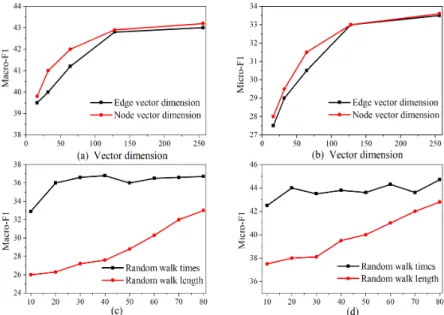
Firstly, the effect of the edge vector dimension and the node vector dimension on NEWEE model are evaluated respectively. The results are shown in Fig. 6 ((a) and (b)). Along with the increase of dimension, the performance of the model is slightly improved since the larger dimension can store more information. Especially for the edge vectors, they contain more information than node vectors. Therefore, the influence of edge vector dimension on NEWEE model is slightly more obvious than that of node vector dimension. In addition, the effect of random walk parameters (walk timesr and walk lengthl) on the model is tested. The results are shown in Fig. 6 ((c) and (d)). With the increase ofr andl value, the performance of the model is improved rapidly and then became relatively stable. The two parameters can also improve the performance of NEWEE model due to that the random walk can traverse more paths from the network to
provide more useful information. However, when the two values increase to a certain value, the provision of information becomes redundant.
Fig. 6.Effect of different parameters on performance of NEWEE model.
4.6 Scalability
This section mainly analyzes the test time of the NEWEE model on different scale networks. We use the Python package NetworkX2to generate Erdos-Renyi
random (ER) networks as the original data of the model. The number of nodes of the networks are set from 100 to 1,000,000, and the node degree is set to 10. Fig. 7 shows the run time of each phase of NEWEE model. It can be seen that the time consumption of NEWEE model has a linear correlation with the number of nodes. Among all the phases, the longest time-consuming part is the random walk of the second phase. This is principally because the NEWEE mod-el needs to calculate the transition probability matrix before random walking, which involves cosine similarity calculation, and is a relatively time-consuming operation. For training the edge vectors in the first stage and training the node vectors (Skip-gram) in the second phase, the model uses negative sampling and asynchronous random gradient descent method to improve efficiency respective-ly. Therefore, these two processes take very little time, especially for the first
2 NetworkX is a Python package for the creation, manipulation, and study of the
structure, dy-namics, and functions of complex networks, and the package can be found at https://networkx.github.io/documentation/stable/
Fig. 7.NEWEE: time vs. number of nodes.
phase, the training speed is very fast. To sum up, the NEWEE model can be applied to large scale real-world networks.
5
Conclusion
This paper presents an unsupervised network representation learning model, called NEWEE, which can not only preserve the information of neighbor n-odes, but also preserve the information of the relationship types between nodes and their neighbors. By performing multi-label classification and link prediction tasks on several real-world networks, our model can achieve excellent perfor-mance. Moreover, we provide a new way to distinguish relationship types with-out labeling data, and it is scalable, and can be applied to large-scale real-world networks.
References
1. Aditya Grover, J.L.: node2vec: Scalable feature learning for networks. In: ACM SIGKDD International Conference on Knowledge Discovery and Data Mining. pp. 855–864 (2016)
2. Bandyopadhyay, S., Kara, H., Biswas, A., Murty, M.N.: Sac2vec: Information net-work representation with structure and content (2018)
3. Belkin, M., Niyogi, P.: Laplacian eigenmaps and spectral techniques for embedding and clustering. Advances in Neural Information Processing Systems14(6), 585–591 (2001)
4. Bourigault, S., Lagnier, C., Lamprier, S., Denoyer, L., Gallinari, P.: Learning social network embeddings for predicting information diffusion pp. 393–402 (2014) 5. Cao, S., Lu, W., Xu, Q.: Grarep: Learning graph representations with global
structural information. In: ACM International on Conference on Information and Knowledge Management. pp. 891–900 (2015)
6. Figueiredo, D.R., Ribeiro, L.F.R., Saverese, P.H.P.: struc2vec: Learning node rep-resentations from structural identity pp. 385–394 (2017)
7. Hamilton, W.L., Ying, R., Leskovec, J.: Inductive representation learning on large graphs (2017)
8. Huang, X., Li, J., Hu, X.: Accelerated Attributed Network Embedding (2017) 9. Jacob, Y., Denoyer, L., Gallinari, P.: Learning latent representations of nodes for
classifying in heterogeneous social networks. pp. 373–382 (2014)
10. Le, T.M.V., Lauw, H.W.: Probabilistic latent document network embedding pp. 270–279 (2014)
11. Leskovec, J., Kleinberg, J., Faloutsos, C.: Graph evolution: Densification and shrinking diameters. Acm Transactions on Knowledge Discovery from Data1(1), 2 (2007)
12. Li, A.Q., Ahmed, A., Ravi, S., Smola, A.J.: Reducing the sampling complexity of topic models pp. 891–900 (2014)
13. Li, J.H., Wang, C.D., Huang, L., Huang, D., Lai, J.H., Chen, P.: Attributed network embedding with micro-meso structure. In: International Conference on Database Systems for Advanced Applications. pp. 20–36 (2018)
14. Mikolov, T., Chen, K., Corrado, G.S., Dean, J.: Efficient estimation of word rep-resentations in vector space. arXiv: Computation and Language (2013)
15. Nallapati, R.M., Ahmed, A., Xing, E.P., Cohen, W.W.: Joint latent topic models for text and citations. In: ACM SIGKDD International Conference on Knowledge Discovery and Data Mining, Las Vegas, Nevada, Usa, August. pp. 542–550 (2008) 16. Neelakantan, A., Shankar, J., Passos, A., Mccallum, A.: Efficient non-parametric estimation of multiple embeddings per word in vector space. Computer Science (2015)
17. Perozzi, B., Alrfou, R., Skiena, S.: Deepwalk: Online learning of social represen-tations. In: ACM SIGKDD International Conference on Knowledge Discovery and Data Mining. pp. 701–710 (2014)
18. Roweis, S.T., Saul, L.K.: Nonlinear dimensionality reduction by locally linear em-bedding. Science290(5500), 2323–2326 (2000)
19. Tang, J., Qu, M., Wang, M., Zhang, M., Yan, J., Mei, Q.: Line: Large-scale infor-mation network embedding2(2), 1067–1077 (2015)
20. Wang, D., Cui, P., Zhu, W.: Structural deep network embedding. In: ACM SIGKD-D International Conference on Knowledge SIGKD-Discovery and SIGKD-Data Mining. pp. 1225– 1234 (2016)
21. Wang, H., Wang, J., Wang, J., Zhao, M., Zhang, W., Zhang, F., Xie, X., Guo, M.: Graphgan: Graph representation learning with generative adversarial nets (2017) 22. Yoshua, B., Aaron, C., Pascal, V.: Representation learning: a review and new
perspectives. IEEE Transactions on Pattern Analysis & Machine Intelligence35(8), 1798–1828 (2013)
23. Zhang, A., Zhu, J., Zhang, B.: Sparse Relational Topic Models for Document Net-works (2013)