Optimal Order Processing Policies for
E-commerce Servers
Yong Tan • Vijay S Mookerjee • Kamran Moinzadeh
University of Washington Business School, Box 353200, Seattle, Washington 98195-3200, USA
University of Texas at Dallas, School of Management, PO Box 830688, JO44 Richardson, TX 75803-0688, USA
University of Washington Business School, Box 353200, Seattle, Washington 98195-3200, USA
[email protected] • [email protected] • [email protected]
The explosive growth in online shopping has provided online retailers impressive opportunities for revenue and profit. At the same time, retailers may lose considerable online business from slow response times at electronic shopping sites. Although increasing server capacity may improve response ti me, the resources and capital needed to do so are clearly not free. In this study, we propose a scheme that can improve a server’s performance under its current capacity. This scheme is based on priority order processing, where the priority of an order depends on the potential revenue that would be generated from the order. The results for single-period analysis show that the benefit from priority processing increases as the server becomes busier.
We have also modeled a multi-period version of the problem, where the demand in a period depends on the Quality of Service (QoS) that buyers receive in the previous period. In multi-period problem, both the server capacity and the order processing policy in each multi-period are determined optimally. Here, it may be optimal for the retailer to sacrifice profit and increase QoS in initial periods in order to increase demand (and revenue) in later periods. Thus, the order processing policy of the server evolves from an emphasis on QoS in initial periods, to one on profit in subsequent periods.
1. Introduction
The last few years have observed an explosive growth in online business. This growth is likely to sustain since the number of Internet users around the world is continues to grow. The Computer Industry Almanac has reported that by the year 2002, 490 million people around the world will have Internet access, that is, 79.4 per 1,000 people worldwide, and 118 people per 1,000 by year-end 2005.
More significantly, Jupiter Communications estimates that online shopping will grow to $78 billion by Year 2003. According to Jupiter Communications, retailers seeking to benefit from the huge online market must design the online experience with a view to establish long term relationships with new online buyers. This is because meeting and exceeding the expectations of new buyers has an effect far beyond the current season; a positive online experience with a specific retailer could go a long way toward securing a future stream of revenues.
In this study, we consider the problem of congestion in e-commerce servers. Our concern is specifically to do with slow response time. A significant statistic here is one provided by Forrester Research Inc. – 66% of all electronic shopping carts are abandoned before a sale is completed. While the abandoning of a cart may occur from reasons that are not related to response time, it is quite clear that slow response time is indeed a significant cause. One study entitled “The Web Is No Shopper’s Paradise,” published in the November 1999 issue of Fortune
magazine states that (Mardesich, 1999):
“Among the 200 Web consumers surveyed for Cognitiative’s (a Net strategy
consulting firm based in San Francisco) quarterly “Pulse of the Customer”
elsewhere was technical problems, including unacceptably slow response times.”
On similar lines, Green (1999) conducted a more detailed survey using 1000 online shoppers to study congestion problems in e-commerce servers. The survey revealed that 28% of the respondents found sites too slow and left, never to return.
An obvious solution to the above congestion problems is to increase server capacity. An interesting case in point here is the e-merchant “800.com,” that sells consumer electronics. After its launch in October 1998, the company tried launched a promotion that offered three movies or three CDs for $1. The promotion worked, perhaps too well. On November 27, 1998 the company’s site was swamped and virtually shut down as hundreds of thousands of customers flocked to the site to obtain cheap movies and CDs. Based on this experience, 800.com now relies on 50 rather than 16 main servers to handle site traffic! However, while adding more servers should clearly alleviate congestion problems; there is no easy formula to determine the optimal number of computers. Furthermore, adding capacity is obviously not free and should be done only if the additional capacity can be economically justified.
A resource neutral solution to the server congestion problem is to improve performance using priority order processing. There could be many dimensions of performance (e.g., average response time, throughput, maximum response time, revenue generated, etc.); our focus here is on two of these measures: profit per unit time and percentage of buyers lost. While profit is an obvious performance measure, the percentage of buyers lost is used to measure Quality of Service (QoS). A buyer’s satisfaction with the electronic shopping process should depend, in part, on whether or not the purchase transaction is successfully completed in a reasonable amount of time. Therefore, the percentage of buyers lost can be used as a measure of the quality of service achieved by a certain electronic site. When profit is the goal of the processing policy,
the amount of processing power assigned to an order depends on two considerations: (a) the potential revenue that would be generated from the order if it is successfully executed, and (b) the probability that the order will be lost because the customer’s delay tolerance is exceeded. On the other hand, when QoS is the goal, the amount of processing power assigned to an order depends only on the probability that the order will be lost.
In deriving the optimal policies, our study spans three research areas: time -shared systems, reneging in queuing theory, and differentiated (or prioritized) services. The concept of time -sharing has been widely adopted in scheduling computer processing (Kleinrock, 1964, 1967, 1976; Stallings, 1997). In time -sharing, processing power can be divided in two ways. The first method, often called “Round-Robin”, is a true time-sharing policy. Each process gets a slice (quantum) of time during which the full capacity of the processor is dedicated to the process. The second method is to divide processing power on a full-time but part-capacity basis. This method, referred to as “Processor-Sharing,” represents the continuous limit of time -sharing where the time slice approaches zero. Kleinrock (1964, 1967) obtained the expected response time (time spent in the system, waiting time plus required processing time) for exponentially distributed arrival and departure (time -shared M/M/1). The waiting time is proportional to the processing time attained; suggesting that round robin systems are more “fair” than sequential queues since the waiting time in sequential systems does not depend on the actual amount of processing incurred on a job. Coffman et al (1970) derived the expression for the waiting time distribution in time-shared systems that was found to deviate from the exponential form that describes the sequential M/M/1 queuing model. Morrison (1985) later found the response time (waiting plus required process time) distribution for M/M/1 processor-sharing systems. Sakata, Noguchi, and Oizumi (1971), and O’Donovan (1974) have extended the results of expected response time to
M/G/1 processor-sharing models.
Customer impatience is a direct source for loss of sales in online retailing; customers quit shopping if the waiting exceeds their tolerance. This phenomenon, termed as queuing with reneging (and balking), has been studied for about 40 years and is still an active research area. Barrer (1957) obtained the results for the queuing problem with impatient customers based on heuristics. Gnedenko and Kovalenko (1989) provided a more rigorous analysis that verifies Barrer’s results. In their studies, they assume a M/M/1 system with either a constant or exponentially distributed reneging time. More detailed studies on M/M/1 system with an exponentially distributed reneging time have been presented by Ancker and Gafarian (1962, 1963). Rao (1968) extended the results to the reneging in M/G/1 systems. In both studies, an exponentially distributed reneging time was assumed. Recent studies are focused on extending to more general queuing systems, for example a GI/G/1 model (Stanford, 1979). In addition, Whitt (1999) studied the reneging problem when customers are informed about anticipated delays. There has been no research to our knowledge that includes the reneging in the time -shared queuing systems. Assaf and Haviv (1990) have studied the strategy of reneging from processor sharing systems. However, the impact of reneging on the queues is not explicitly modeled.
Kleinrock (1967) introduced the notion of priority processing for computer processors and derived the expected waiting time for different priority classes with exponentially distributed processing time. O’Donovan (1974) showed that the result holds even for M/G/1 processor-sharing systems. Similarly in networking, the vision of providing differentiated services has been around for well over a decade (Turner, 1986). Future packet networks will likely support Quality of Service in order to provide a full array of services (Aiello et al, 2000). Research in this area is becoming increasingly popular, as new technology makes implementation possible. Other studies
have been focused on economic side, namely pricing for providing priority services in communication networks as well as in other settings (Marchand, 1974).
In this study, we propose and analyze optimal order processing policies that can be used by e-commerce servers to improve performance. We also provide a variety of analytical and numerical results that prescribe how E-retailers should best run their servers to achieve their performance goals. We also study a multi-period version of the server congestion problem, where both the server capacity and the processing policy in each period are optimally determined. In the multi-period problem, we consider QoS externalities; demand in a given period depends on the QoS achieved in the previous period. The multi-period problem is solved using dynamic programming. The results from the multi-period analysis can provide guidelines for e-retailers to adjust the order processing policy over time. For example, the analysis reveals that e-retailers should initially pay more attention to QoS. However, as the customer base of an e-retailer matures, profit-oriented order processing policies should be pursued.
The rest of the paper is organized as follows. Sections 2 and 3 are dedicated to the analysis of optimal server operating policies. A single period model is presented in Section 2 whereas Section 3 extends the single period model to a multi-period one. Numerical results are presented and practical implications are discussed. Section 4 provides a summary of results and offers directions for future research.
2. The Model
In this section, we set up the basic model where the demand is assumed to be stationary. This is a single period problem. E-retailers first determine and acquire the optimal capacity that remains unchanged for the rest of the planning horizon.
2.1 Assumptions and Preliminaries
We characterize orders arriving at an E-commerce server by their values. The predicted final purchase value of an order, h, follows a value distribution, f(h). One way to predict the final purchase value is to use the customer’s historic data, for example, an average value (or a moving average). After each purchase, the data can be modified and a new average value can be calculated for use for the next visit. For a first time buyer, a typical value, such as the market average for all new buyers can be used. This study assumes a “static” policy, i.e., each customer is assigned an estimated value that remains unchanged throughout the course of shopping. In a more sophisticated model, the predicted final value can vary “dynamically,” for example, by utilizing information about the value of items in the shopping cart. These and other methods (e.g., data mining techniques) can be applied. A dynamical policy offers more accurate value prediction, however with the cost of extra computational overhead. A static policy estimates the value “offline”, therefore does not consume online resources but may suffer from inaccuracy. We will attempt to address this tradeoff question in subsequent studies.
The total arrival rate of orders is λ, this is the number of orders per unit time. We assume that orders arrive according to a Poisson process, which represents real situation quite well (Moe and Fader, 2001). Each order requires certain amount of time to be processed. A typical online shopping process involves various activities, for example, browsing, searching, adding items to shopping cart, and checkout. For a static policy, we ignore the details of involved shopping activities (as these information are not used to update the predicted value), and instead define the required processing time as the total time that an order receives processing from the server including all shopping activities. The required processing time for orders with value h is assumed to be exponentially distributed with an average time τ(h), which is a function of the value.
Therefore the overall processing time distribution for all orders is described by the hyper-exponential distribution, or a linear combination of hyper-exponential distributions with different means. The assumption of exponential processing time simplifies policy analysis. We have not attempted to generalize this assumption; however, it is a good approximation for time -shared systems where it has been shown (Sakata, Noguchi, and Oizumi, 1971; O’Donovan, 1974) that several important results (such as mean delays) depend only on the mean processing time and not on the distribution. In general, average required processing time is a non-decreasing function of the value. In our model, any function form of τ(h) can be used.
Impatient customers may quit shopping if the time spent exceeds their tolerance for waiting. We define the tolerance level of a shopper in terms of average time in the server, w(h), that is, buyers with the value h are willing to wait for a random time that is exponentially distributed (Ancker and Gafarian, 1962) with a mean w(h). It is likely that customer impatience varies during the course of shopping. Similarly for a static policy, we suppress this variation and adopt an average level over various points of the shopping process. The impatience of an on-line shopper is modeled using an analogy from the “express lane” in a traditional grocery store. Typically store express lanes provide faster service to customers with relatively fewer items. The implicit assumption here is that customers with fewer items may be less tolerant of delays; more generally, the tolerance level of a customer is assumed to depend in some way on the number of items that the customer intends to purchase. In our model, the delay tolerance w(h) can be any function of h; however, it is plausible that w(h) is increasing in h.
Similar to the scheduling of a computer processor, server capacity is shared by orders in the server. The sharing scheme in a typical e-commerce server is based upon “Round-Robin” time-sharing. Specifically, an order is given a slice of processing time, say Q, when it enters the
processing unit of the server. It exits from the system if it finishes the desired processing during this allotted time. Otherwise, it goes back to the end of the queue and waits for its next turn. Round-Robin scheduling is better than a sequential scheduling (in which customers are served one at a time) because sequential scheduling may waste capacity while waiting for a client’s response.
We introduce the prioritized processing by assigning a weight gk (gk ≥ 0) for orders in
priority class-k so they receive processing time, gkQ. This scheme was first proposed by
Kleinrock (1967). The priority of an order is determined by the potential final value of the purchase that a buyer makes. In this study, we limit ourselves to the case where there are an infinite number of classes. This allows us to focus on the properties of priority scheme without involving complicated problem of assigning orders to classes. The processing weight gk becomes
continuous and is a function of value h, g(h). Offering discrete classes may be optimal if the cost of implementing the policy is considered. A model for discrete classes has been published elsewhere (Tan, 2000).
As mentioned earlier, customers will abandon their shopping cart (or renege) if they have been made to wait for too long. We have solved a queuing problem that incorporates reneging in a priority-based time-sharing system. The result is summarized in the following proposition. Proposition 1 The loss function density (defined as number of customers lost per unit time per unit value), l(h), for orders with value h, is
(
)
(
)
( ) ) ( ) ( 1 ) ( ) ( 1 ) ( ) ( ) ( f h h g h w h g h h g h h l λ τ τ + + + = ,where g(h) must satisfy,
(
)
(
( ) 1)
( ) ( ) ( ) 1 ) ( ) ( 1 ) ( ) ( ) ( = + + +∫
∈H h dh h f h g h w h g h h g h g h h w λ τ τ , (1)and H is the set of all possible values.
The proof is presented in the Appendix, where the proofs for all the propositions, corollaries and lemmas can be found.
In the next section, we introduce a multi-period version of this model where capacity choices can be made at the beginning of each period. In this section, however, we have assumed that capacity can be chosen once, at the beginning of the period. The effect of increasing server capacity is to reduce the required processing time of an order:
C h
h) ( )/
( τ0
τ = , (2)
where τ0(h) is the processing time for a standard unit of capacity, and C is the server capacity. A more powerful server has a larger value of C, and therefore orders can be processed faster. There is a cost associated with acquiring capacity. We assume a linear cost, γC, where γ is the unit cost (normalized to per unit time). The linear form can be justified as in most cases capacity can be additive, for example, if more servers are added. We ignore the fixed cost, as it does no t affect our results.
2.2 Profit-focused Policy
The total expected revenue (per unit time) can be written as,
(
)
∫
∈ − = H h dh h l h f h S λ ( ) ( ) . (3)A retailer’s objective is to choose capacity and processing weight such that the expected profit per unit time is maximized. Explicitly, we define an E-retailer’s problem:
(
)
(
)
f h dh C h Cg h w h g h h h Cg h w C h g H h C h g π =∫
τ + + λ −γ ∈ ) ( ) ( ) ( 1 ) ( ) ( ) ( ) ( ), ( max 0 ), ( , subject to(
)
(
)
∫
∈ + + + = H h dh h f h Cg h w h g h h g h g h h w ) ( ) ( ) ( 1 ) ( ) ( ) ( 1 ) ( ) ( ) ( 1 0 0 λ τ τ , (4) H h h g( )≥0, ∀ ∈ .Equation 4 is identical to Equation 1 with capacity C explicitly expressed. The solution to this problem is given in the following proposition:
Proposition 2The optimal processing weight allocation is
∉ ∈ − + − + + = ; , 0 ; , 1 ) ( ) ( 1 1 ) ( 1 1 ) ( / ) ( 1 1 ) ( 2 / 1 * S S H h H h h h w h h h h w h g τ ψ τ τ
where ψ is the Lagrange multiplier associated with Equation 4, and the serviceable set HS is
defined as, ≥ ∈ = h H h h h HS , ) ( : ψ τ .
The optimal capacity is,
(
)
(
)
∫
∈ + + + = H h dh h f h g h w h g h h g h g h h w C ( ) ) ( ) ( 1 ) ( ) ( ) ( 1 ) ( ) ( ) ( * * * 2 * * τ τ γ λψ .Proposition 2 indicates that there is a revenue realization threshold defined by hτ(h)≥ψ ; only orders with revenue realization above this threshold receive processing capacity. The revenue realization threshold is rate at which an order’s revenue is realized. The value of ψ can be obtained by substituting the expressions of g*(h) and C* in Equation 4. The problem is reduced to solving for ψ and C*. The following corollary provides bounds for numerical search. Corollary 1 The optimal capacity C* satisfies the following inequalities:
* * S C ≤ ≤γ ψ .
order will get processed if it can recover the cost of capacity. The system can also afford to admit some orders whose values are below the cost of capacity. The second inequality guarantees a non-negative profit; representing the individual rationality condition for the retailer.
We have shown the following comparative static results hold. Corollary 2 For the optimal processing weight allocation g(h),
i.
(
)
0 ) ( / ) ( * > ∂ ∂ h h h g τ ; ii.(
)
0 ) ( / ) ( ) ( * < ∂ ∂ h h w h g τ .Orders with higher rate of revenue realization (i.e., the h/τ(h) ratio) receive more processing time. The ratio w(h)/τ(h)measures a customer’s patience level. Orders with a higher value of this ratio (more patient buyers) can tolerate more delay and hence receive less processing time.
Figure 1 shows the optimal processing weight, g*(h), for linear processing time and waiting tolerance: τ(h)=0.7+0.3h, and w(h)=1+0.5h. Here we assume that capacity is fixed, so only the threshold ψ needs to be calculated. The value distribution is uniform, namely, f(h) = 1 for h∈
[0, 1]. g*(h) increases with value h as the ratio h/τ(h) is an increasing function of h while )
( / ) (h h
w τ decreases with h. However in Figure 2, with nonlinear forms of τ(h)=0.3+0.7h3, andw(h)=0.5+0.8h2, g*(h) is not monotonic. It turns out that the ratio h/τ(h) peaks around the value h ≈ 0.6. This example shows the importance of gathering information on customer purchasing behavior (e.g., the delay tolerance); a higher value (h) alone does not warrant higher priority.
0 0.2 0.4 0.6 0.8 0 0.2 0.4 0.6 0.8 1 h g * (h ) λ = 3 λ = 7
Figure 1. Optimal processing weight, g*(h), plotted as a function of value, h, for linear processing time and waiting tolerance.
0 0.1 0.2 0.3 0.4 0 0.2 0.4 0.6 0.8 1 h g * (h )
Figure 2. Optimal processing weight, g*(h), plotted as a function of value, h, for non-linear processing time and waiting tolerance.
Corollary 3 With the change of demand, λ,the following results hold:
i. 0 * > ∂ ∂ λ π ; ii. 0 * > ∂ ∂ λ C ; iii. *>0 ∂ ∂ C ψ λ , if * a0 C > ψ ,
where the expression for the coefficient a0 is given in the proof.
When the total demand increases, the expected profit (i) will also increase. This can be achieved by adding more capacity (ii). The server becomes more discriminating by raising the threshold (iii) when the threshold exceeds a certain level. The threshold ψ/C* translates to value threshold hc, * 0 ) (h C h c c ψ τ = .
Figure 3 shows the value threshold hc as a function of demand, with the same parameter setting
priority orders are more likely to complete. Otherwise, the capacity will be adjusted optimally with demand, without much increase in the degree of differentiation.
0 0.1 0.2 0.3 0.4 0.5 0 2 4 6 8 10 λ hc Optimal Capacity Constant Capacity
Figure 3. Value threshold for serviceable orders, hc, plotted as a function of demand,
λ for fixed capacity and capacity determined optimally. 0 0.1 0.2 0.3 0.4 0.5 0.6 0 0.2 0.4 0.6 0.8 1 h g * (h ) Profit-focused QoS-focused Uniform
Figure 4. Optimal processing weight, g*(h), plotted as a function of value, h, for profit-focused, QoS-oriented, and uniform (non-differentiated) policies.
Corollary 4 With the change of capacity cost, γ,the following results hold:
i. 0 * < ∂ ∂ γ π ; ii. 0 * < ∂ ∂ γ C ; iii. *>0 ∂ ∂ C ψ γ .
It is intuitive that when the cost of capacity increases, the expected profit (i) and capacity (ii) will drop. When the cost of capacity increases, the server becomes more discriminating (iii) by raising the threshold.
2.3 QoS-focused Policy
In this subsection, we consider a policy that focuses on the Quality of Service (QoS). We define the QoS as the number of lost orders per unit time, regardless of their order value. The
E-retailers’ problem becomes,
∫
∈ ≡ H h h g L l(h)dh min ) ( , (5)where l(h) is the loss function density, given in Proposition 1. The optimal processing allocation can be obtained similarly,
≥ < − + − + + = . ) ( , 0 ; ) ( , 1 ) ( ) ( 1 1 ) ( 1 ) ( / ) ( 1 1 ) ( 2 / 1 * c c c h h h h w h h h w h g τ τ τ τ τ τ τ τ
The processing time threshold τc can be found by substituting the above expression in
Equation 1. It is obvious from the above equation that orders more processing will be assigned less processing time. More patient buyers (with higher w(h)/τ(h) ratio) also receive less processing time. The value threshold hc is given by τ(hc)=τc. Assuming τ(h) increases with the
value h, orders with value above the threshold hc will not receive any processing capacity.
We next compare three policies: profit-focused, QoS-focused, and uniform. The uniform policy is a non-discriminating policy where g(h) is a constant. Here, linear forms of
h
h) 0.7 0.3
( = +
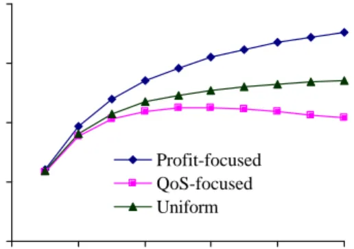
τ and w(h)=1+0.5h are used, and the capacity C is set to be 1. Figure 4 clearly shows the difference between profit-focused and QoS-oriented policies. QoS policies favor low value customers, as orders from such buyers consume less processing time. Figure 5 plots the expected revenue (or profit as the capacity is fixed). The QoS-focused policy is the worst performer as it favors low value orders (with shorter processing time). For the Profit-focused policy, the improvement in revenue increases when server becomes busier (higher λ). Figure 6 plots the loss ratio of customers, L/λ, a measure for the quality of service. The QoS-focused policy is most effective in the middle range of demand, since L/λ converges to 0 as λ → 0, and 1 as λ →∞, for all policies.
0 0.2 0.4 0.6 0.8 0 2 4 6 8 10 λ Revenue ( S * ) Profit-focused QoS-focused Uniform
Figure 5. Sales, plotted against demand, λ, for profit-focused, QoS-oriented, and uniform (non-differentiated) policies. 0.5 0.6 0.7 0.8 0.9 1.0 0 2 4 6 8 10 λ L/λ Profit-focused QoS-focused Uniform
Figure 6. QoS (percent lost customers, L/λ), against demand, λ, for profit-focused, QoS-oriented, and uniform policies.
3. Multi-Period Model
In Section 2, we presented various polices that attempt to optimize an E-retailer’s profit in a single period. However, retailers often value their customer base more than immediate profit. This consideration is not without merit since lost customers rarely come back. This suggests that during initial periods, the value of orders should be paid less importance so as to build a solid customer base. In this section, we propose a multi-period model that includes feedback on quality of service. Specifically, the quality of service that customers receive in a period affects the demand in the next period. E-retailers are allowed to vary capacity to match the demand.
We add an index, j for the period, to the notation used in the previous section. We start with the loss function density lj(h) in the j-th period. The expression for lj(h) is the same as the one
shown in Proposition 1 with subscripts for the period j wherever necessary. The expected number of buyers lost per unit time in the j-th period, Lj, is calculated using Equation 5 and lj(h).
We model the demand in the (j + 1)-th period in the following way:
(
j j)
jj j
j+ =L ⋅p + λ −L ⋅r
due to successful purchases, for example through “word of mouth”. Equation 6 can also be expressed in terms of the expected percentage of buyers lost, Lj/λj, a measure of QoS.
E-retailers are allowed to adjust capacity, both upwards and downwards; implying that we accommodate situations in which capacity can be rented. We assume that the cost of acquiring capacity is proportional to the capacity added, namely, γj(Cj −Cj−1), where Cj is the capacity in
the j-th period. Similarly as in Equation 2, we have τj(h)=τ0j(h)/Cj. Since hardware cost typically decreases with time, the coefficient γj is assumed to decrease from period to period.
Without loss of generality, we assume that the demand becomes stationary in the N-th period. E-retailers have N opportunities to adjust capacity, after which the capacity remains unchanged from the N-th period onwards. The discounted profit is,
(
)
N N j N j j j j j j j j C h g S C C δ S δ γ δ π δ − + − − =∑
∞∑
= = − − − 1 ) ( max 1 1 1 1 1 ), ( ,where δ is the discount factor; and g(h) and C are short hands for the processing weight and capacity vectors. The profit, πj = SN, for j ≥ N + 1, because the operating policy and capacity
remain unchanged from the N-th period onwards. The discounted profit can be represented by a finite horizon formulation,
∑
= − N j j j 1 1π
δ , where πNis redefined as,
) ( 1− − − −1 = N N N N N C C S γ δ π .
We can solve this multi-period problem using the method of dynamic programming (Dreyfus and Law, 1977), more specifically, backward induction. Let us define
(
l l l l)
N j l l j l C h g j j j C C g h C l l ), ( ; , max ) , ( 1 ), ( 1 − = − − ≡∑
Π λ δ π λ ,which can be obtained recursively using the demand generation model as specified by Equation 6. Πj(λj,Cj−1) is the maximum discounted profit starting from the j-th period. It depends on the demand arriving in this period, λj, and the capacity carried over, Cj−1. This allows us to write the
recursive relation,
(
, ; ( ),)
( , ) max ) , ( 1 1 1 ), ( 1 j j j j j j j j C h g j j j C C g h C C j j + + − − ≡ + ⋅Π Π λ π λ δ λ , (7)where Π0(λ0) is the objective function.
We first introduce the following lemma.
Lemma 1 The effect of carry-over capacity on the maximum discounted profit is described as below, j j j C =γ ∂ Π ∂ −1 .
This result is intuitive as more existing capacity reduces the cost of capacity in the current period, and consequently increases the discounted profit. Now we are in a position to characterize the optimal policies.
Proposition 3 The optimal processing weight allocation in the j-th period (j < N) is
∉ ∈ − + − + + = ; , 0 ; , 1 ) ( ) ( 1 1 ) ( 1 ) ( / ) ( 1 1 ) ( 2 / 1 * S j S j j j j j j j j H h H h h h w h h h w h g ψ τ κ τ
where the serviceable value set S
j H is defined as,
{
j j j}
S j h h h H H = :κ ( )≥ψ , ∈ , and 1 ) ( ) (h h j 1 r p τ λ δ τ κ − ∂ Π ∂ + = + . (8)The optimal capacity is,
(
)
(
)
∫
∈ + + + + − = j H h j j j j j j j j j j j j j j f h dh h g h w h g h h g h g h h w C ( ) ) ( ) ( 1 ) ( ) ( ) ( 1 ) ( ) ( ) ( * * * 2 * 1 * τ τ δγ γ ψ λ .For periods j ≥ N, the processing weight and capacity are given by Proposition 2 with the
effective unit capacity cost, (1− δ)γN.
As displayed in Equation 8, this policy seems to combine the profit-focused and QoS-oriented policies for the single period problem; the factor κj(h) is a linear combination of two
ratios, h/τ(h) and 1/τ(h). The relative weight of this combination is determined by the discount factor δ, and two parameters rj and pj that determine the demand growth. This controls the
evolution of the operating policy from a QoS-focus at the beginning to a profit focus when the demand is steady.
In the following, we present some numerical demonstrations. Given the results described in Proposition 3, in each period, we numerically evaluate ψj and C*j, and make use of Corollary 5.
Corollary 5 The following recursive relation holds,
1 1 2 * ) ( ) ( ) ( + + ∈ ∂ Π ∂ + = ∂ Π ∂
∫
j j j H h j j j j j j p dh h f h g h w j λ δ ψ λ .The computation procedure is as follows. We start from the N-th period where the policy in this period is described by Proposition 2. The recursion in Corollary 5 is then applied in the previous period to obtain the optimal policy in the (N-1)-th period, using Proposition 3.
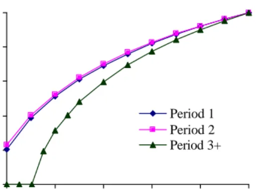
0 0.2 0.4 0.6 0.8 1 0 0.2 0.4 0.6 0.8 1 h gj * (h )/ gj * (1) Period 1 Period 2 Period 3+
Figure 7. Optimal processing weights (normalized), gj*(h)/gj*(1), plotted as a
function of value, h, for discounting factor δ = 0.3. 0 0.2 0.4 0.6 0.8 1 1.2 0 0.2 0.4 0.6 0.8 1 h gj * (h )/ gj * (1) Period 1 Period 2 Period 3+
Figure 8. Optimal processing weights (normalized), gj*(h)/gj*(1), plotted as a
function of value, h, for discounting factor δ = 0.6.
Figures 7 and 8 plot the optimal processing allocations for N = 3; rj = 2, pj = 0.2;
h h
j( ) 0.7 0.3
0 = +
τ ,wj(h)=1+0.5h; γ1= 0.4, γ2= 0.35, γ3= 0.3; and uniform value distribution
for 0 ≤h ≤ 1. The processing allocation is purely profit-focused from the third period onwards. E-retailers with higher δ are less discriminating as is evident from a lower value threshold hc. A
higher value of discount factor δ indicates that the E-retailer is more concerned about the long-term. There is heavier capacity investment in the initial period to accommodate more customers. As δ increases, the policies in the initial periods becoming less discriminating, or more QoS-oriented, due to the influence of future demand growth.
Figure 9 shows the optimal capacity increments in three periods. We assume the capacity remains unchanged from the third period onwards. E-retailers with low value of δ invest in capacity in the initial period and maintain a more or less a constant capacity level, even with the decreasing cost of capacity. They focus on profit making even in the initial periods. This results in poor QoS, and therefore there is no growth in demand. E-retailers with higher δ invest heavily
sees a small increase or even a decrease in capacity. Partly, the demand growth is yet to take full effect so the slightly increased or even decreased capacity can sustain the same level of QoS. Also, the acquiring of capacity can be postponed to the third period that has a lower capacity cost. Recall that the effective unit capacity cost is (1 − δ)γN. It decreases with discount factor δ,
therefore we expect the optimal capacity increment in the third period to increase with δ.
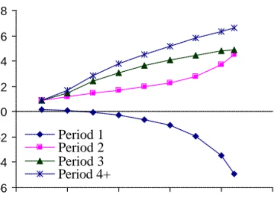
Figure 10 shows that the profits in the second, third, and fourth periods increase with discount factor. This is because of the increased customer base (or demand). In the second period, releasing of capacity gives a slightly faster increase of profit with higher δ. The difference between the third period and periods from the fourth onwards is the cost of capacity. It is apparent that E-retailers with longer horizons (higher δ) suffer more in the initial periods, from heavy investments in capacity that are aimed at improving QoS.
-6 0 6 12 18 0 0.2 0.4 0.6 0.8 1 δ ∆ Cj * Period 1 Period 2 Period 3
Figure 9. Optimal capacity increments, ∆Cj*,
plotted against discounting factor, δ.
-6 -4 -2 0 2 4 6 8 0 0.2 0.4 0.6 0.8 1 δ π j * Period 1 Period 2 Period 3 Period 4+
Figure 10. Profit in each period, πj*, plotted as
a function of discounting factor, δ.
4. Conclusions and Future Research
In this study, we propose an order processing scheme that improves the performance of an E-commerce site. This scheme is based on priority order processing, where the priority of an order
depends on the potential value of the order. We present the model and the results for a single-period. It is shown that the benefit from priority processing increases as the server becomes busier.
We have also modeled a multi-period problem, where the demand in a period depends on the Quality of Service (QoS) that buyers receive in the previous period. It is observed that the retailer usually loses money in the first period in order to provide better service and growth in future demand. The operating policy of the server evolves from a QoS-focused one in initial periods, to a profit-focused one in subsequent periods. In multi-period problem, the server capacity planning in each period is determined optimally.
The current study involves one server (or treats multiple servers as a single server). It is of practical importance to study the load-balancing problem. This is a two-level problem. Each server will be optimized using priority scheme, conditional on an optimal amount of traffic directed to the server. Another interesting extension is to control or influence the value distribution, f(h). This can be achieved using appropriate incentive schemes, such offering on the spot discount to buyers that may otherwise leave. Finally, we are working on the analysis of dynamic order processing policies that allow the priority of an order to vary during the course of shopping, especially in response to a more accurate prediction of the final value, and the delay tolerance.
References
Aiello, W. A., Mansour, Y., Rajagopolan, S., and Rosen, A., “Competitive Queue Policies for Differentiated Services,” Proceedings of INFOCOM, 2000.
Ancker, C. J. and Gafarian, A. V., “Queuing with Impatient Customers Who leave at Random,”
Operations Research, 11, pp. 88-100, 1963.
Ancker, C. J. and Gafarian, A. V., “Some Queuing Problems with Balking and Reneging – II,”
Operations Research, 11, pp. 928-937, 1963.
Assaf, D. and Haviv, M., “Reneging from Processor Sharing Systems and Random Queues,”
Mathematics of Operations Research, 15, 129-138, 1990.
Barrer, D. Y., “Queuing with Impatient Customers and Indifferent Clerks,” Operations
Research, 5, 644-649, 1957.
Barrer, D. Y., “Queuing with Impatient Customers and Ordered Service,” Operations Research, 5, 650-656, 1957.
Coffman, E. G., Muntz, R. R., and Trotter, H., “Waiting Time Distributions for
Processor-Sharing Systems,” Journal of the Association for Computing Machinery, 17(1), pp. 123-130, 1970.
Dreyfus, S. E. and Law, A. M., The Art And Theory Of Dynamic Programming, Academic Press, New York, 1977
Gnedenko, B. V. and Kovalenko, I. N., Introduction to Queuing Theory, Birkäuser, Boston, 1989.
Green, H., “The Great Yuletide Shakeout,” Business Week, pp. EB 18-28, November 1, 1999. Kleinrock, L., “Analysis of a Time -Shared Processor,” Naval Research Logistics Quarterly, 11,
59-73, 1964.
Kleinrock, L., “Time-shared Systems: A Theoretical Treatment,” Journal of the Association for
Computing Machinery, 14(2), pp. 242-261, 1967.
Kleinrock, L., Queueing Systems: Volume 2, Computer Applications, Wiley, New York, 1976. Marchand, M. G., “Priority Pricing,” Management Science, 20(7), pp. 1131-1140, July 1974. Mardesich, J., “The Web Is No Shopper’s Paradise,” Fortune, pp. 188-198, November 8, 1999. Moe, W. W. and P. S. Fader, “Modeling Online Store Visit Patterns as a Measure of Customer
Satisfaction,” Wharton School Working Paper, 2001.
Applied Mathematics, 45, 152-167, 1985.
O’Donovan, T. M., “Direct Solutions of M/G/1 Processor-Sharing Models,” Operations
Research, 22, pp. 1232-1235, 1974.
Rao, S. S., “Queuing with Balking and Reneging in M / G / 1 Systems,” Metrika, 12, pp. 173-188, 1968.
Sagan, H., Introduction to the Calculus of Variations, McGraw-Hill, New York, 1969.
Sakata, M., Noguchi, S., and Oizumi, J., “An analysis of the M/G/1 Queue under Round-Robin Scheduling,” Operations Research, 19, 371-385, 1971.
Stallings, W., Operating Systems: Internals and Design Principles, Prentice Hall, New Jersey, 1997.
Stanford, R. “Reneging Phenomena in Single Channel Queues,” Mathematics of Operations
Research, 4, 162-178, 1979.
Tan, Y., “Value-based Design of Electronic Commerce Servers,” Doctoral Dissertation, University of Washington, 2000.
Turner, J. S., “New Directions in Communications,” IEEE Communications Magazine, 10, 1986. Weinstock, R., Calculus of Variations, McGraw-Hill, New York, 1952.
Whitt, W., “Improving Service by Informing Customers about Anticipated Delays,”
Management Science, 45(2), pp. 192-207, 1999.
Appendix
Proof of Proposition 1
Discrete Classes. Let us first solve the discrete version of the problem. Assume that there are N
priority classes; class-k orders have arrival rate λk, processing rate µk and reneging rate νk. Let Ek
be the expected number of class-k orders in the system in the steady state.
We follow the method used by Kleinrock (1964). Introduce a tagged order (assume it is one of the priority class-k orders). Each order in class-k is given a time slice (quantum) of gkQ, where
Q is infinitesimal. The cycle time is the duration between two consecutive ejects of the tagged order from the server, namely
Q g QE g k N i i i +
∑
=1 .With a probability µkgkQ, an order of class-k will finish needed processing and exit from
the system during the processing time gkQ allocated to this order. After a cycle, expected number
of class-k orders will be
(
)
k k N i i i k k N i i i k k k kg Q E g QE g Q gQE g QE + − + + −∑
∑
= =1 1 1 µ λ ν .The first term is the expected number of class-k orders returning to the system. The second term is the expected number of class-k orders arriving during a cycle. The third term is the expected number of class-k orders reneging during a cycle.
In the steady state, the above expression should be the same as Ek. Therefore we get
k k N i i i k k N i i i k k k kg E g E g g E g E + − + =
∑
∑
= =1 1 ν λ µ , or ) ( ) ( G g g G g E k k k k k k k + + + = ν µ λ ,where the constant
∑
∑
= = + + + = = N i i i i i i i i N i i i G g g g G g E g G 1 1 ( ) ) ( ν µ λ . (A1)The above constant can be solved self-consistently. The expected loss function for class-k orders is then
) ( ) ( G g g G g E L k k k k k k k k k k + + + = = ν µ ν λ ν .
This is the expected number of class-k orders lost per unit time.
Existence of Unique Positive Value of G.Let’s rewrite Equation A1 as
∑
= = − + + + = N i i i i i i i i G G g g g G g G 1 0 ) ( ) ( ) ( ν µ λ ϕ .The function ϕ(G) has N negative poles at G =−(µi /νi +1)gi, and (N – 1) negative zeros (roots)
in between these poles. For the region where G≥0,
∑
= > + = N i i i i ig 1 0 ) 0 ( ν µ λ ϕ ,and ϕ(∞)→−∞. Its second derivative,
(
( ))
0 2 ) ( 1 3 2 2 2 < + + − =∑
= N i i i i i i i i i G g g g dG G d ν µ ν µ λ ϕ .Therefore ϕ(G) is a concave function over G ≥0, with ϕ(0) > 0 and ϕ(∞)→−∞. It must cross zero once and only once at a positive value of G.
Rescaling and Continuous Limits. The existence of a positive G allows us to rescale the weight vector, explicitly,
k
k G g
g → .
The rescaled gk must satisfy Equation A1 (where G is set to 1). With the continuous value
distribution f(h), required processing time τ(h) (inverse the service rate), and waiting time w(h), we can take continuous limit with respect to value, while retaining the discreteness of priority classes. For orders that have values in the interval [h, h + dh], if belonging to priority class-k, the loss function becomes,
dh h f g h w g h g h dh h l k k k k ( ) ) ( ) 1 )( ( ) 1 )( ( ) ( λ τ τ + + + = ,
Proof of Proposition 2
We adopt the method of calculus of variations (Sagan, 1969; Weinstock, 1952) that is widely used to find the functional form that will optimize a given objective function.
Optimal Processing Allocation. We start by writing the Lagrange of Problem 1,
∫
∈ = H h dh C h g( ), ) ( L L ,where, the integrand, or Lagrange density, is
(
)
(
)
(
( ) 1)
( ) ( ) ( ) ( ) ( ). ) ( ) ( 1 ) ( ) ( ) ( 1 ) ( ) ( ) ( 1 ) ( ) ( ) ( ) ( ) ), ( ( h g h h f h g h w h g h h g h g h h w h f h g h w h g h h h g h w h h g ξ λ τ τ λ ψ λ τ + + + + − + + + = Lψ is the Lagrange multiplier for constraint given by Equation 4. ξ(h) is the Lagrange multiplier density for constraints g(h)≥0 ,∀h∈H . It is positive if g(h) = 0, and zero if g(h) > 0. The first variation yields,
(
)
(
)
(
)
(
)
(
( ) ( ) 1 ( ) ( ))
( ). ) ( ) ( 1 ) ( ) ( ) ( ) ( ) ( ) ( ) ), ( ( 2 2 2 h h g h w h g h h h g h w h g h h f h h w h g h h g ξ τ ψ τ λ τ + + + − × + + = ∂ ∂L (A2)Setting the above equation to zero, we get, if g(h) > 0,
(
)
(
2 2)
) ( ) ( 1 ) ( ) (h g h w h g h h=ψ τ + + ; (A3) and if g(h) = 0, . ) ( ) ( ) ( ) ( − = h h h w h f h τ ψ λ ξ Obviously, if , ) ( ψ τ h ≥ hξ(h) becomes zero, therefore the corresponding constraints are non-binding. The above results are summarized in Proposition 2. The value of Lagrange multiplier ψ can be solved by substituting the expression of g*(h) into constraint given by Equation 4.
Second Variation and Concavity. Let’s perform the second variation around g*(h). This is done by differentiating Equation A2 with respect to g(h) and substituting in Equation A3. We have, for g*(h) > 0,
(
( ) 1)
( ) ( ) ) ( ) ( ) ( ) ( 2 ) ( ) ), ( ( * * ) ( * ) ( 2 2 h g h w h g h h f h h w h g h h g h g h g + + − = ∂ ∂ = τ λ τ ψ L .This is strictly negative as ψ > 0. Therefore, the solution g*(h) yields maximum value for the profit function π.
For the solution that lies on the boundary, i.e. g*(h) = 0, the profit will decrease, at a rate – ξ(h), if g(h) is increased from g*(h) = 0.
Optimal Capacity. The optimal capacity can be obtained by differentiating the Lagrange, explicitly,
(
)
(
)
(
)
(
)
( ) 0 ) ( ) ( 1 ) ( ) ( ) ( ) ( ) ( 1 ) ( ) ( ) ( 2 0 0 = − + + + + = ∂ ∂∫
∈ γ λ τ ψ τ H h dh h f h Cg h w h g h h g h w h h g h g h h w C L .Substituting in Equation A3, the above expression can be simplified to,
(
)
(
)
λ γ τ τ ψ = + + +∫
∈H h dh h f h g h w h g h h g h g h h w C ( ) ( ) 1 ( ) ( ) ( ) ) ( 1 ) ( ) ( ) ( * * * 2 * * . (A4)Solving Equations A3, A4, and constraint given by Equation 4, we can find the optimal policy described by g*(h), C*, and ψ.
In the following we show the capacity solved above is optimal. First, taking derivative of Equation 4, and combined with Equation A3, we have,
11 12 * * a a C C ψ ψ = ∂ ∂ .
The second derivative of Lagrange with respect to C is,
− = ∂ ∂ − = ∂ ∂ 11 2 12 22 2 * * * 12 22 2 * 2 2 a a a C C C a a C C ψ ψ ψ ψ L . (A5)
The coefficients are,
(
)
(
)
∫
∈ + + + + = H h fdh w g g w g g w a λ τ τ τ 3 * * 2 2 * 2 * 11 ) 1 ( 2 ) ( ) 1 ( ;(
)
(
)
∫
∈ + + + − + − + = H h fdh w g g w g g w g g g w a λ τ τ τ τ 3 * * 2 * 3 * 2 * 2 * 2 4 * 12 ) 1 ( 2 ) 1 ( ) ( 2 ) 1 ( ) ( ) 1 ( ;(
)
(
)
∫
∈ + + + − + − + = H h fdh w g g w g g w g g g w a λ τ τ τ τ 3 * * 2 2 * 3 * 3 * 2 * 2 4 * 22 ) 1 ( 2 ) 1 ( ) ( 4 ) 1 ( ) ( 4 ) 1 ( .We find that coefficients a11, a12, and a22 have the following properties:
1. a11>0;
2. a11>a12 >a22;
3. a11+a22 <2a12.
Then, it is straightforward to show that Equation A5 is negative. If a22 <0, it is obvious that 0 2 12 22 11a −a < a ; while if a22 ≥0, we have 2 a11a22 ≤a11+a22 <2a12.
Proof of Corollary 1
Since g*(h) is nonnegative, from Equation A4, we have,
(
)
(
)
γ ψ λ τ τ γ ψ = + + + ≥∫
∈H h dh h f h g h w h g h h g h g h h w C ( ) ) ( ) ( 1 ) ( ) ( ) ( 1 ) ( ) ( ) ( * * * * * .(
)
λ γ τ γ * * * * * ) ( ) ( ) ( 1 ) ( ) ( ) ( ) ( 1 S dh h f h g h w h g h h g h hw C H h = + + ≤∫
∈ .where S* is the expected revenue.
Proof of Corollary 2
Part i is straightforward, and,
(
)
( ) 0 ) ( 1 1 ) ( 1 1 2 ) ( ) ( / ) ( ) ( * 2 1/2 * < + − + − = ∂ ∂ − h h w h h h g h h w h g τ τ ψ τ .Proof of Corollary 3
Part i. The derivative of the expected profit with respect to the demand is, according to envelope theorem,
(
)
∫
(
(
)
(
)
)
∈ + + + − = ∂ ∂ = ∂ ∂ H h dh h f h g h w h g h h g h h h g h w C h g ( ) ) ( ) ( 1 ) ( ) ( 1 ) ( ) ( ) ( ) ( ), ( * * * * * * * τ ψτ π λ λ π .Substituting Equation A3, we have,
(
( ))
( ) 0 ) ( * 2 * > = ∂ ∂∫
∈H h dh h f h g h w ψ λ π .Parts ii and iii. Taking derivatives (with respect to λ) of Equations 4 and A4, and making using of Equation A3, we get,
λ λ λ ψ ψ 1 * * 12 11 = ∂ ∂ − ∂ ∂ C C a a ; ψ γ λ λ λ ψ ψ * * * 22 12 C 1 C C a a = ∂ ∂ − ∂ ∂ ;
Solving these equations, we obtain,
− − − − = ∂ ∂ γ λ ψ λ ψ λ * 11 12 22 12 2 * 1 a a C a a a a a C .
This becomes positive if 22 12 12 11 0 * a a a a a C − − = > γ ψ .
Corollary 2 and properties of coefficients a11, a12, and a22 immediately render,
0 12 * 11 22 11 2 12 * * > − − = ∂ ∂ λ ψ γ λ λ a C a a a a C C .
Proof of Corollary 4
Part i. To show that the expected profit decreases with the increased capacity cost, we find that,
(
*( ), *)
* 0 * < − = ∂ ∂ = ∂ ∂ C C h g π γ γ π .Parts ii and iii. Similarly we take derivatives (with respect to γ) of Equations 4 and A4, this yields, 0 * * 12 11 = ∂ ∂ − ∂ ∂ γ γ ψ ψ C C a a ; ψ γ γ ψ ψ * * * 22 12 C C C a a − = ∂ ∂ − ∂ ∂ .
Solving these two equations simultaneously, we have,
0 22 11 2 12 12 11 * − > − = ∂ ∂ a a a a a C ψ γ ; 0 * 22 11 2 12 * 11 * < − − = ∂ ∂ ψ γ C a a a C a C .
Proof of Lemma 1
Proof of Proposition 3
We follow Equation 7, and write the j-th period problem,
(
, ; ( ),)
( , ) max 1 1 1 ), (h C j j j j j j j j gj j C − g h C + + C Π ⋅ +δ λ λ π subject to:(
)
(
)
∫
∈ + + + = j H h j j j j j j j j j j j dh h f h g C h w h g h h g h g h h w ) ( ) ( ) ( 1 ) ( ) ( ) ( 1 ) ( ) ( ) ( 1 0 0 λ τ τ ;(
)
(
)
∫
∈ + + + + + = j H h j j j j j j j j j j j j j f h dh h g h w h g h p h g h r h g h w ) ( ) ( ) ( 1 ) ( ) ( 1 ) ( ) ( ) ( ) ( 1 λ τ τ λ ; h h gj( )≥0, ∀ .Similar to single period problem, we can define a Lagrange,
(
)
(
)
(
)
(
)
(
)
, ) ( ) ( ) ( ) ( ) ( 1 ) ( ) ( 1 ) ( ) ( ) ( ) ( ) ( ) ( ) ( 1 ) ( ) ( ) ( 1 ) ( ) ( ) ( 1 ) , ( ), ( ; , 1 0 0 0 0 1 1 1∫
∫
∫
∈ ∈ + ∈ + + − + − + + + + + + + + − + Π ⋅ + = j j j H h j j H h j j j j j j j j j j j j j j H h j j j j j j j j j j j j j j j j j j j dh h g h dh h f h g C h w h g h p h g h r h g C h w dh h f h g C h w h g h h g h g h h w C C h g C ξ λ λ τ τ χ λ τ τ ψ λ δ λ π Lwhere, ψ j, χj, and ξj(h) are Lagrange multipliers (or density). The first variation gives,
(
)
(
2 2)
) ( ) ( 1 ) ( ) ( ) (r p h g h w h g h h+χj j − j =ψ jτ j j + + j j , (A6) where, 1 1 + + ∂ Π ∂ = j j j λ δ χ .(
)
(
)
1 1 * * * 0 * 2 * 0 * ( ) ) ( ) ( 1 ) ( ) ( ) ( 1 ) ( ) ( ) ( + + ∈ − = ∂ Π ∂ − = + + +∫
j j j j j H h j j j j j j j j j j j C dh h f h g C h w h g h h g h g h h w C j δγ γ δ γ λ τ τ ψ .Similar to the single-period problem, the derivation of this result utilizes the solution *( )
h gj , given by Equation A6, and Lemma 1. Note that, if one requires that the capacity is non-decreasing, (namely, Cj ≥Cj−1), a positive number, εj, (the Lagrange multiplier) should be
subtracted from the right hand side of the above expression.
Proof of Corollary 5
Using the definition of Πj(λj,Cj−1), given by Equation 7, and the envelope theorem, we have,
(
)(
)
(
)
∫
∈ + + − + + + = ∂ Π ∂ j H h j j j j j j j j j j j j j j j j j j dh h f h g h w h g h h g h w p h g h r h h g h w ) ( ) ( ) ( 1 ) ( ) ( ) ( ) ( 1 ) ( ) ( ) )( ( ) ( * * * * * τ ψ χ τ χ λ .