Sharif University of Technology
Scientia IranicaTransactions E: Industrial Engineering www.scientiairanica.com
An evolutionary algorithm for supplier order allocation
with fuzzy parameters considering linear and volume
discount
M. Sou Neyestani
a, F. Jolai
b;and H.R. Golmakani
a a. Department of Industrial Engineering, University of Tafresh, Tafresh, Iran.b. Department of Industrial Engineering, College of Engineering, University of Tehran, Tehran, Iran. Received 30 May 2012; received in revised form 3 July 2013; accepted 19 May 2014
KEYWORDS Multi-period
multi-product supplier order allocation; Linear discount; Volume discount; Jimenez method; PSO;
GA.
Abstract. In this research, the supplier order allocation problem is investigated. The problem is when one buyer wants to allocate required products to pre-selected suppliers. Allocation is considered under some constraints, such as capacity, delivery rate, linear discount and volume discount. Objectives of the model are towards maximizing the total value of purchases, minimizing the total cost of purchases and minimizing the total number of defective products purchased. We propose a Multi-Objective Mixed Integer Non-Linear (MOMINL) model for multi-period supplier order allocation in situations where suppliers oer discounts. In practice, some information, such as buyer demand and supplier delivery rate, is uncertain, so, fuzzy sets are applied to handle uncertainty. Since PSO and GA are the most eective methods for nding a good solution to a dicult Multi-Objective Problem (MOP), a multi-objective optimization algorithm, based on PSO and GA (MOPSOGA), is developed to solve the model and give a set of Pareto optimal solutions. The eciency of the Pareto Archive obtained from the algorithm is evaluated based on spacing and diversity metrics.
c
2015 Sharif University of Technology. All rights reserved.
1. Introduction
Two of the most important decisions which should be made in the eld of purchasing management are sup-plier selection and order allocation [1]. Order allocation involves determining the amount of purchased items from each supplier in each planning period. According to the results of periodic evaluations, the manager allocates orders to pre-selected suppliers. In real situations, suppliers often oer discounts, a motivation for using discount schemes stemming from the fact
*. Corresponding author. Tel.: +98 21 88021067; Fax: +98 21 88013102
E-mail addresses: [email protected] (M. Sou Neyestani); [email protected] (F. Jolai);
[email protected] (H.R. Golmakani)
that it tends to encourage buyers to procure larger quantities. From a coordination perspective, it has been shown that both the buyer and the supplier can realize higher overall prots if discount schemes are used to set transfer prices [2,3]. Also, because some input information, such as buyer demand and supplier delivery rate, is uncertain, we use a procedure proposed by Jimenez et al. [4] for handling uncer-tainty.
This paper is organized as follows: In Section 2, the literature is reviewed. Multi-Objective Problems are noted in Section 3. In Section 4, a Multi-Objective Mixed Integer Non-Linear model (MOMINL) is con-structed. In Section 5, a MOPSOGA to solve the model is described, and, in Section 6, we analyze the performance criteria of this model. The specications of test problems used to compare the performance of
the proposed algorithm are explained in Section 7, and the results of the experiments are presented in Section 8. Conclusions and desired future research areas are presented in Section 9.
2. Literature review
Kawtummachai et al. [5] proposed an algorithm for the supplier order allocation problem. The objective of their model was minimizing the total purchasing cost, while maintaining a specied service level. Xia et al. [6] developed an integrated approach of ANP, improved by rough set theory and MOMI programming, for the problem to simultaneously determine the number of suppliers to employ and the order quantity allocated to these suppliers in cases of multiple sourcing and multi-product with multi-criteria, supplier capacity constraints, and regarding volume discount. Liao et al. [7] developed a MOP model for the problem in cases of single item, multi-period supplier selection and lot sizing with inconstant demand. They applied the genetic algorithm to solve the model. Ma et al. [8] presented an integrated MINL programming model for supplier selection under uncertain demand and a volume discount environment problem. The objective of their model was to maximize manufacturer expected prot, subject to both manufacturer and supplier capacities. Mohammad Ebrahim et al. [3] considered the supplier selection problem in the presence of three dierent discounts, all units, incremental, and total business volume, and introduced a mathematical model for a single item. In addition, constraints, such as purchasing supplier capacity and demand, were taken into consideration in the model. Due to the complexity of the problem, they proposed a Scatter Search Algorithm (SSA) to solve it. Demirtas and Ustun [9] combined ANP and MOMIL programming models to solve the order allocation problem, using the Reservation Level Driven Tchebyche Procedure. They minimized the total defect rate and the total cost of purchasing and maximized TVP. Jolai et al. [10], in continuation of the work by Demirtas and Ustun [9], considered a supplier selection problem for multi-products. Sawik [11] considered the order allocation problem for custom parts among suppliers in a make-to-order environment. He presented single objective and multi-objective mixed integer models, based on price, quality and reliability of on-time delivery in quantity, or a business volume discount oered by the suppliers, to solve the problem.
Order allocation decisions can be largely inu-enced by alternative supplier pricing schemes, and, to the best of our knowledge, the eect of discount on allocation strategy in multi-period and multi-product have not been considered in any previous research. So, the major contribution of this paper is in extending
prior research models and in considering the eect of linear and volume discount on an order allocation problem in multi-period and multi-product supplier selection. Because of the complexity of our model, we developed the MOPSOGA algorithm to solve it and nd a set of Pareto optimal solutions.
3. Multi-objective optimization
Most real world problems have several conicting objectives. The term Multi-Objective Optimization Problem (MOP) is used to broadly classify problems with more than one objective. A typical multi-objective minimization problem with decision variables and objectives is shown in Eq. (1):
Minz = f(x) = (f1(x); f2(x); :::; fm(x)) ; (1)
where x 2 Rnand z 2 Rm. A rather practical approach
to deal with multi-objective problems is to nd a set of solutions, called a Pareto set, instead of nding a single solution. A solution is said to be Pareto-optimal if it is not dominated by any other feasible solution. Denition 1. In a Pareto optimal solution, solution a is said to dominate solution b, if, and only if;
1. fi(a) fi(b) 8i = 1; 2; :::; m;
2. fi(a) < fi(b) 8i = 1; 2; :::; m:
Solutions that dominate other solutions, but do not dominate themselves, are called non-dominated solu-tions.
Denition 2. Vector a is a globally Pareto-optimal solution if vector b does not exist, such that b dominates a. The set of all Pareto-optimal solutions is called the Pareto-optimal set. The corresponding images of the Pareto-optimal set in the objective space are called the Pareto-optimal frontier [12,13].
4. Mathematical model
In the following section, we develop a Multi-Objective Mixed Integer Non-Linear model to allocate order be-tween pre-selected suppliers. The indices, parameters, and decision variables of the model are as follows: Notation:
Indices
i = 1; 2; :::; n Index of suppliers which oer linear discount discounts;
j = 1; 2; :::; n Index of products; t = 1; 2; :::; T Index of time periods; r = 1; 2; :::; R Index of discount interval.
Parameters
m1 Number of suppliers who oer linear
discount discounts;
m2 Number of suppliers who oer volume
discount discounts;
Djt Demand of the product j in period t;
Oit Order cost for supplier i in period t;
qijt Defect rate of supplier i for product j
in period t;
Qj Buyer's maximum acceptable defect
rate of product j;
Vijt Capacity of supplier i for product j in
period t;
hjt Holding cost of product j in period t;
Pijt Purchasing price of product j from
supplier i in period t (supplier i oer linear discount);
P P minijt Minimum purchasing price of product
j from supplier i in period t if Xijt
equals Vijt (supplier i oers volume
discount);
P P maxijt Maximum purchasing price of product
j from supplier i in period t if Xijt
equals L (supplier i oer volume discount);
CDirt Coecient of volume discount for
supplier i in interval r and period t; V P Pirt Volume of purchased products from
supplier i in interval r and period t; LBirt Lower bound of volume discount
supplier i in interval r and period t; UBirt Upper bound of volume discount
supplier i in interval r and period t; Aijt; Bijt Linear discount coecient for supplier
i in period t and for product j; DTijt On-time delivery rate of supplier i for
product j in period t;
DT Bj Buyer's minimum acceptable delivery
rate for product j;
Wit The overall score of supplier i in period
t;
L Minimum order quantity if an order is to be placed on supplier i for product j in period t.
Decision variables
Xijt Number of the product j ordered from
supplier i in period t;
Yit 1 if an order is placed on supplier j in
period t, 0 otherwise;
Ijt Inventory of product j carried over
from period t to t + 1(Ij0= 0);
XYirt 1 if an order is placed on supplier i
in discount interval r and period t, 0 otherwise.
4.1. Defuzzication of MOMINLP model for order allocation problem
In this model, there are three objectives: total cost of purchase, total value of purchase and total number of defective product purchases. The problem is to determine the amount of products allocated to each supplier in each period, in order to satisfy buyer demand. We assume that the buyer wants to allocate the demand of n products between m pre-selected suppliers in T periods. The assumptions used in constructing the model are as follows:
Demand of each product in each period is fuzzy.
Linear discount and volume discount are considered in making allocation decisions.
In order allocation, delivery rate is also considered a constraint.
On-time delivery rate of each supplier for each product in each period is fuzzy.
The buyer can purchase the required quantity from multiple suppliers.
The buyer is purchasing for multi-period.
The objective functions and constraints of this model are as follows:
4.2. Objective functions 4.2.1. Total cost of purchase
The sum of the periodic material cost, periodic order cost, and holding cost make up the Total Cost of Purchase. Instead of using a xed cost, a linear discount and volume discount are considered. Under volume discount assumption, each supplier oers price discounts on total business volume, not on the quantity or variety of products purchased from them. In addition, under a linear discount, each supplier, i, discloses a linearly declining per unit price for each product, j, in each period, t, in the quantity, Xijt,
dened as (Bijt+ AijtXijt). Therefore, the following
equation is proposed:
MinZ1= T
X
t=1
Xm1
i=1 n
X
j=1
(Bijt+ AijtXijt)Xijt
+ Xm
i=m1+1
R
X
r=1
(1 Cdirt)VPPirt
+Xm
i=1
OitYit+ n
X
j=1
hjtIit
4.2.2. Total value of purchase
Wit and Xijt denote the priority values of the
pre-selected suppliers and the number of purchased units from the ith supplier in period t, respectively. The supplier's priority values are used as coecients of the Total Value of Purchase to allocate order quantities among the pre-selected suppliers, such that the total value of the purchases becomes maximized. The following equation is presented to show the objective function:
MaxZ2= T
X
t=1 m
X
i=1 n
X
j=1
WitXijt: (3)
4.2.3. Total number of defective product purchase the buyer expects to minimize the number of defective products purchased at each period for improving the quality of purchased products. This need is shown as follows:
MinZ3= T
X
t=1 m
X
i=1 n
X
j=1
qijtXijt: (4)
4.3. Constraints
The important constraints of the supplier order alloca-tion problem are volume and linear discount, inventory control, material balance, demand, supplier capacity, minimum order quantity, and delivery rate.
4.3.1. Volume discount constraints
In this type of discount, suppliers oer price discounts, which depend on the total value of sales volume over a given period of time. The volume, VPPirt, from
supplier i in period t, should be in an appropriate discount interval, r, of the discount pricing schedule and only in one interval. This is formulated in the following:
R
X
r=1
V P Pirt= n
X
j=1
PijtXijt
i = m1+ 1; :::; m; t = 1; 2; :::; T; (5)
LBirtxyirt V P Pirt< UBirtxyirt
i = m1+ 1; :::; m; r = 1; 2; :::; R;
t = 1; 2; :::; T; (6)
R
X
r=1
xyirt 1
i = m1+ 1; :::; m; t = 1; 2; :::; T: (7)
4.3.2. Linear discount constraint
Each supplier, i = 1; 2; :::; m1, discloses a linearly
declining per unit price for each product, j, in each period, t, in quantity Xijt. Prices between P P minijt
and P P maxijt are gained by solving Constraints 8
and 9.
Aijt= P P minijtV P P maxijt ijt L
i = 1; 2; :::; m1; j = 1; 2; :::n; t = 1; 2; :::; T; (8)
Bijt= P P maxijt L
P P minijt P P maxijt
Vijt L
i = 1; 2; :::; m1; j = 1; 2; :::; n; t = 1; 2; :::; T:
(9) 4.3.3. Demand constraint
The sum of the acceptable products of type, j, received from all suppliers in each period, t, plus carried quantities from the preceding period should satisfy buyer demand for that product in that period. This is formulated as follows:
Jj(t 1)+ m
X
i=1
(1 qijt)Xijt ~Djt
j = 1; 2; :::; n; t = 1; 2; :::; T: (10) 4.3.4. Material balance equation
This constraint is to make sure that the material balance for each product, j, in the period, t, is equal to the material balance of the product in the previous period, plus the wholesale purchase of the product subtracts from the demand of the product.
Jj(t 1)+ m
X
i=1
(1 qijt)Xijt ~Djt
j = 1; 2; :::; n; t = 1; 2; :::; T: (11) 4.3.5. Capacity constraint
Considering that supplier i can produce up to Vijt
units of product, j, in period, t, and that, in its order quantity of product, j, in period, t, Xijt should be
less than or equal to its capacity, which is shown in Relations (12) and (13).
Xijt YitVijt i = 1; 2; :::; m;
j = 1; 2; :::; n; t = 1; 2; :::; T; (12) Xijt LYit i = 1; 2; :::; m;
4.3.6. Delivery rate constraint
According to Dickson [14], delivery rate is an important factor in supplier selection and is considered in many papers, so, we have considered it a constraint in the model in the following formulation:
m
X
i=1
1 DT~ ijt
Xijt ~Djt(1 DT Bj)
j = 1; 2; :::; n; t = 1; 2; :::; T: (14) 4.3.7. Non-negatively and binary constraints
the following decision variable, Xijt, is a non-negative
variable, and Yitand XYirtare binary variables:
Xijt 0 i = 1; 2; :::; m; j = 1; 2; :::; n;
t = 1; 2; :::; T; (15) Yit2 f0; 1g i = 1; 2; :::; m; t = 1; 2; :::; T; (16)
XYirt2 f0; 1g
i = m1+ 1; :::; m; j = 1; 2; :::; n;
t = 1; 2; :::; T: (17) 4.4. Defuzzication of fuzzy MOMINL model If we suppose demand and delivery time to be fuzzy triangular numbers, ~Djt = (D1; D2; D3) ~DTijt =
(DT1; DT2; DT3), the crisp model, according to the
model of Jimenez et al. [4], can be written by the following:
MinZ1= T
X
t=1
Xm1
i=1 n
X
j=1
(Bijt+ AijtXijt)Xijt
+
m
X
i=m1+1
R
X
r=1
(1 Cdirt)V P Pirt
+Xm
i=1
OitYit+ n
X
j=1
hjtIit
; (18)
MaxZ2= T X t=1 m X i=1 n X j=1
WitXijt; (19)
MinZ3= T X t=1 m X i=1 n X j=1
qijtXijt; (20)
R
X
r=1
V P Pirt= n
X
j=1
PijtXijt
i = m1+ 1; :::; m; t = 1; 2; :::; T; (21)
LBirtxyirt V P Pirt< UBirtxyirt
i = m1+ 1; :::; m; r = 1; 2; :::; R;
t = 1; 2; :::; T; (22)
R
X
r=1
xyirt 1 i = m1+ 1; :::; m; t = 1; 2; :::; T;
(23)
Aijt= P P minVijt P P maxijt ijt L
i = 1; 2; :::; m1; j = 1; 2; :::; n; t = 1; 2; :::; T;
(24)
Bijt= P P maxijt L
P P minijt P P maxijt
Vijt L
i = 1; 2; :::; m1; j = 1; 2; :::; n; t = 1; 2; :::; T;
(25)
Jj(t 1)+ m
X
i=1
(1 qijt) Xijt
ED~jt
2 + (1 )E ~ Djt
1
j = 1; 2; :::; n; t = 1; 2; :::; T; (26)
Ijt= Ij(t 1)+ m
X
i=1
(1 qijt) Xijt
ED~jt
2 + (1 )E ~ Djt
1
j = 1; 2; :::; n; t = 1; 2; :::; T; (27) Xijt YitVijt
i = 1; 2; :::; m; j = 1; 2; :::; n; t = 1; 2; :::; T; (28) Xijt LYit
i = 1; 2; :::; m; j = 1; 2; :::; n; t = 1; 2; :::; T; (29)
m
X
i=1
((1 )EDT~ ijt
2 + E
~ DTijt
1 ) 1
Xijt
ED~jt
2 + (1 )E1D~jt
(DT Bj 1)
i = 1; 2; :::; m; t = 1; 2; :::; T; (30) Xijt 0 i = 1; 2; :::; m; j = 1; 2; :::; n;
Yit2 f0; 1g i = 1; 2; :::; m; t = 1; 2; :::; T; (32)
XYirt2 f0; 1g i = m1+ 1; :::; m;
j = 1; 2; :::; n; t = 1; 2; :::; T: (33) In the above model, denotes the minimum acceptable feasibility degree of the decision vector and belongs to [0,1], according to [4]. In this research, we assume that = 0:35.
5. Applying MOPSOGA to solve the problem As mentioned before, in MOP, it is better to nd a set of solutions, called a Pareto set, instead of nding a single solution, which is as diverse as possible in an objective space [12].
5.1. GA and PSO
GA is a population-based heuristic search algorithm that starts with an initial set of solutions (individuals) which are then evolved toward better solutions via certain genetic operators, such as selection, mutation and crossover. Selection is a fundamental operator by which individual genomes are chosen from a population for later breeding. The crossover operator combines in-formation from two solutions of the current population in such a way that the two solutions for the next pop-ulation resemble each parent. The mutation operator alters or mutates one chromosome by changing one or more variables in some way or by some random amount to form one ospring [12,15].
PSO is also a most recent evolutionary tech-nique inspired by the ocking behavior of birds. It is initialized with a population of random solutions and searches for an optimal by updating generations. The potential solutions, or particles, move through the problem space by following the current optimum particles. The position of particle i is presented as Xi = (Xi1; Xi2; :::; XiD); each particle keeps a memory
of its previous best position, P best, represented as Pi = (Pi1; Pi2; :::; PiD), and a velocity along each
dimension represented as Vi = (Vi1; Vi2; :::; ViD). The
position of the particle with the best tness value in the search space, designated as g, and the p vector of the current particle, are combined to ad-just the velocity along each dimension. That ve-locity is then used to compute a new position for the particle. In other words, the particle swarm optimizer keeps track of the overall best value, and its location, obtained thus far by any particle in the population, which is called pbest(Pid), and each particle
keeps track of the best solution, called gbest(Pgd),
attained within a local topological neighborhood of particles:
Vid=! Vid+ c1 r1 (Pid Xid)
+ c2 r2 (Pgd Xid); (34)
Xid = Xid 1+ Vid; (35)
where Vidis the velocity of the particle, Xid is the
cur-rent position of the particle, ! is the inertia factor, c1
determines the relative inuence of the cognitive com-ponent, c2determines the relative inuence of the social
component, r1 and r2 are random numbers uniformly
distributed in the interval [0,1], ! controls the inuence of the previous velocity on the new velocity, and c1
and c2are positive constants, determining the relative
inuence of the social and cognitive components [16]. 5.2. MOPSOGA
We developed a multi-objective optimization algo-rithm based on PSO and GA to solve the model. The algorithm uses a xed-sized population (P opsize)
and starts with a randomly generated population. At each iteration of the algorithm, the population is divided into two parts and developed with the PSO and GA separately. First, the population is evolved over a certain number of generations by PSO (KeepPercent). Second, (P opsize KeepPercent)
indi-viduals are generated by implementing GA operators, such as selection, crossover and mutation. Finally, the (P opsize KeepPercent) individuals are combined with
the (KeepPercent) particles to form a new population for the next iteration.
To update the position and velocity of particles in MOPSO, we use Eqs. (34) and (35), as mentioned above. We also use NSGA-II, described by Deb et al. [17], to select parents in MOGA. In NSGA-II, crowding distance measure is used as a tiebreaker in a selection technique, called the crowded tournament selection operator, which randomly selects two chro-mosomes from the population. If the chrochro-mosomes are in the same non-dominated front, the chromosome with a higher crowding distance is the winner [7,18]. In MO, a Pareto based approach is used to check two solutions, so, after each iteration of MOPSO and MOGA, we should update the Pareto solution archives. We use the contents of this archive as a nal report of MOPSOGA. The steps of the MOPSOGA algorithm are briey shown as a Pseudo code in Table 1, and a ow chart of this algorithm is shown in Figure 1.
6. Performance metrics
Several performance metrics are available for testing the quality of multi-objective solutions in the liter-ature. Most of these metrics are concentrated on two issues: First, maximizing the distance between the Pareto frontier and the actual Pareto frontier generated by an algorithm; the distance is called the
Table 1. Pseudo code used for MOPSOGA. Begin
Initialize parameters: KeepPercent, c1; c2; !, Crossoverpercent, Mutationpercentand Popsize;
i = 1; j = 1;
while j <= Max itera do //Iteration loop starts here Generate popsizerandom solutions;
Calculate objectives function; Update Pareto solution;
while i <= KeepPercentdo //MOPSO evolution
Update position and velocity of the particles; Calculate objectives function;
Update Pareto solution; i = i + 1;
end //end of MOPSO evolution i = KeepPercent;
while i <= Popsize do //MOGA evolution Parent selection (using crowded distance); Implement crossover and mutation operators; Calculate objectives function;
Update Pareto solution; i = i + 1;
end //end of MOGA evolution
Combine particles obtained by MOPSO and individuals obtained by MOGA and form Popsize particles;
j = j + 1;
end // Iteration loop ends here End
diversity metric. Secondly, minimizing the smoothness of solution distribution; the smoothness is called the spacing metric.
6.1. Diversity
The diversity metric was introduced by Van Veldhuisen and Lamont [19]. It evaluates the distance between the obtained non-dominated solutions by an algorithm and the actual Pareto optimal solutions (assuming we know these solutions). This distance is calculated by the following equation:
Diversity = pPn
i=1d2i
n ; (36)
where n is the number of non-dominated solutions and di is the Euclidian distance (depending on the
number and actual value of objectives) between each non-dominated solution and the nearest one in the Pareto optimal set. It is clear that Diversity=0 means all solutions are in the Pareto frontier. The values greater than zero indicate the relative distance between
the obtained solutions and actual Pareto frontier. Based on the literature, more diversity leads to better solutions.
6.2. Spacing
The spacing metric was introduced by Schott [20]. It is a tool to measure the uniformity of the spread of solutions. The distance variance of each point in the current solution set to its closest neighbor is calculated by the following equation:
SP = v u u t 1
n 1
n
X
i=1
(d di)2; (37)
where n, the number of non-dominated solutions, is obtained by the MOPSOGA algorithm, and d is the mean value of all di. Note that SP = 0 means all
non-dominated solutions are spaced equally from each other. Based on the literature, less spacing leads to better solutions.
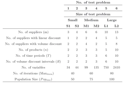
Table 2. Specication of 6 test problems; number of iteration and population size. No. of test problem
1 2 3 4 5 6
Size of test problem
Small Medium Large
S1 S2 M1 M2 L1 L2
No. of suppliers (m) 3 4 6 6 10 13
No. of suppliers with linear discount 1 2 2 4 5 5 No. of suppliers with volume discount 2 2 4 2 5 8
No. of products (n) 2 2 3 3 5 10
No. of time periods (T ) 2 2 3 3 6 10
No. of volume discount intervals (R) 2 2 2 3 6 10 No. of variables 34 44 99 135 750 2410 No. of iterations (Maxitera) 40 60 80
Population Size (P opsize) 50 75 100
Figure 1. Flow-chart of the MOPSOGA.
7. Test problem specications
Based on our knowledge, the proposed model has not been considered so far, and we have not found another solution method to compare its performance with the proposed MOPSOGA. In order to evaluate the performance of the proposed model, we have surveyed the model in six test problems. The specications of each test problem are described in detail in Table 2.
For all test problems, the following assumptions hold:
1. We have three segments of customers, S = 3.
2. We have solved all problems based on two values for k, k = 0:2; 0:14.
3. All problems are solved based on three dier-ent values of s, 1 = (0:4; 0:35; 0:25), 2 =
(0:45; 0:33; 0:22), and 3= (0:5; 0:30; 0:20).
4. Holding cost is constant and is equal to 20.
8. Experimental evaluations
The proposed model is applied to six test problems (small, medium and large size). In order to evalu-ate the eciency of the proposed model, sensitivity analysis is done on PSO and GA parameters. Four dierent input value combinations for six PSO and GA parameters are set, including c1; c2; !, keep percent,
mutation percent and crossover percent. Random test problems with dierent size type are generated and solved by MOPSOGA for each combination of parameters.
The proposed algorithm is coded in Matlab pro-gramming language and all the test problems are solved by it with dierent parameter values. The acquired
Table 3. Result of MOPSOGA and sensitivity analysis on 6 test problems.
Algorithm parameters setting GA: crossover percent=60%, mutation percent=10% PSO: C1 = 1:5, C2= 2:5, W = 0:999, keep percent =30%
No. of test problem Problem size Pareto Diversity Spacing Elapsed time
1 S1 498 4.0331e+004 0.8753 255.445719
2 S2 317 3.6458e+004 1.3652 123.557192
3 M1 448 3.6186e+004 1.1691 691.498439
4 M2 680 4.8651e+004 0.6989 1096.913247
5 L1 673 7.9582e+004 0.8990 1529.621017
6 L2 569 1.2249e+005 0.7775 1936.027078
Algorithm parameters setting GA: crossover percent=40%, mutation percent=20% PSO: C1 = 2, C2= 2, W = 0:7, keep percent =40%
No. of test problem Problem size Pareto Diversity Spacing Elapsed time
1 S1 435 3.3194e+004 0.8113 379.243945
2 S2 298 2.9305e+004 1.1422 99.216689
3 M1 440 3.4815e+004 1.2671 382.296274
4 M2 520 4.5768e+004 0.8171 719.657635
5 L1 759 7.6406e+004 0.7997 1957.886543
6 L2 900 1.6673e+005 0.8621 2160.341653
Algorithm parameters setting GA: crossover percent=50%, mutation percent=0% PSO: C1= 2:5, C2= 1:5, W = 0:2, keep percent =50%
No. of test problem Problem size Pareto Diversity Spacing Elapsed time
1 S1 368 3.4253e+004 0.8390 181.225394
2 S2 298 3.5734e+004 1.1825 139.112256
3 M1 339 3.0170e+004 1.1751 258.183892
4 M2 574 3.5649e+004 0.7848 604.069026
5 L1 442 5.8436e+004 0.8314 455.769588
6 L2 367 1.0606e+005 0.7579 656.037240
Algorithm parameters setting GA: crossover percent=20%, mutation percent=20% PSO: C1= 3, C2= 1, W = 0:85, keep percent =60%
No. of test problem Problem size Pareto Diversity Spacing Elapsed time
1 S1 266 2.5244e+004 0.8296 113.292985
2 S2 491 4.2870e+004 1.1460 243.701100
3 M1 393 3.2501e+004 1.0359 251.528521
4 M2 397 3.5333e+004 0.7545 225.536679
5 L1 433 6.5011e+004 0.9412 490.530861
6 L2 630 1.3169e+005 0.8271 1679.733900
Pareto, spacing, diversity and elapsed time values for each test problem are shown in Table 3.
The numbers of Pareto solutions found by MOP-SOGA in small, medium, large and very large size problems are represented in Figures 2 to 5. Three axes, X, Y and Z, exist, which show the objective functions 1, 2 and 3, respectively. As observed, Pareto solutions
move to maximize objective function 2 and minimize objective functions 1 and 3.
The numbers of Pareto solution obtained for each test problems are presented in Figure 6; the horizontal axis shows the number of variables and the vertical axis shows the number of Pareto solution. The average complexity time for dierent test problems is also
Figure 2. Pareto solutions for problem with 4 suppliers, 2 products and 2 periods.
Figure 3. Pareto solutions for problem with 6 suppliers, 3 products and 3 periods.
Figure 4. Pareto solutions for problem with 13 suppliers, 10 products and 10 periods.
presented in Figure 7; the horizontal axis shows the number of variables, and the vertical axis shows the elapsed time. As can be observed, an increase in the size of the problem increases the solution time of the MOPSOGA algorithm.
Figure 5. Pareto solutions for problem with 10 suppliers, 5 products and 6 periods.
Figure 6. Pareto-optimal solutions found by algorithm for a 4-sensivity analysis and 6-test problems.
Figure 7. Average computational times for dierent problems.
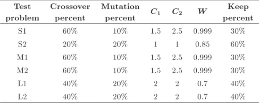
Based on the results, there is no signicant dierence among the results for the spacing metrics and it could be ignored. On the contrary, diversity metrics show a signicant dierence among the results. Since the number of Pareto solutions is supposed to be the response variable, the following conclusions are obtained. The best results yield for the problems where the parameters crossover percent, mutation percent c1; c2; !, and keep percent are set as shown in
Table 4. Best parameters setting for each test problem. Test
problem
Crossover percent
Mutation
percent C1 C2 W
Keep percent
S1 60% 10% 1.5 2.5 0.999 30%
S2 20% 20% 1 1 0.85 60%
M1 60% 10% 1.5 2.5 0.999 30%
M2 60% 10% 1.5 2.5 0.999 30%
L1 40% 20% 2 2 0.7 40%
L2 40% 20% 2 2 0.7 40%
9. Conclusion
The problem of allocating orders among suppliers properly, in multiple supplier environments, is more complicated than the supplier selection problem. Split-ting orders to the selected suppliers has become a major challenge for buying rms, especially when suppliers oer multiple products and discounts.
Very little attention has been paid in the lit-erature to decisions on assigning order quantities to suppliers in cases of discounted costs. So, in this research, a MOMINL model is proposed to nd the optimum quantities among the qualied suppliers. Our model considers a multi-period, multi-product supplier order allocation problem under fuzzy demand, fuzzy delivery rate, and linear and volume discounts. In this model, we seek to maximize the total value of purchase, minimize the total cost of purchase, and minimize the total number of defective products purchased, simultaneously.
Due to the complexity of the problem, and since PSO and GA algorithms are the most eective methods for nding a good solution to a dicult Multi-Objective Problem (MOP), a multi-objective optimization al-gorithm, based on PSO and GA (MOPSOGA), has been developed to solve the model and obtain a set of Pareto optimal solutions. The performance of the proposed method was evaluated by six test problems, and sensitivity analysis was undertaken on PSO and GA parameters. The eciency of the Pareto Archive obtained from the algorithm is evaluated based on diversity and spacing metrics. The calculated diversity and spacing show the good performance of the solution. It was observed that algorithm parameters values have more eect on the number of the Pareto solution and diversity, and a lower eect on spacing. The experimental results have indicated that by an increase in the size of the problem, the MOPSOGA algorithm takes more time to solve it. So, for future research, other evolutionary algorithms could also be applied, and comparisons with the proposed algorithm could be carried out. Furthermore, instead of fuzzy demand and delivery rate, stochastic or time dependent demand and delivery rate could be considered.
Acknowledgments
The authors would like to thank the reviewers of this paper whose constructive comments were helpful in its revision.
References
1. Ghodsypour, S.H. and O'Brien, C. \A decision sup-port system for supplier selection using an integrated analytic hierarchy process and linear programming", Int. J. of Production Economics, 56-57, pp. 199-212 (1998).
2. Burke, G.J., Carrillo, J. and Vakharia, A.J. \Heuristics for sourcing from multiple suppliers with alternative quantity discounts", European Journal of Operational research, 186(1), pp. 317-329 (2008).
3. Mohammad Ebrahim, R., Razmi, J. and Haleh, H. \Scatter search algorithm for supplier selection and order lot sizing under multiple price discount environ-ment", Advances in Engineering Software, 40(9), pp. 766-776 (2009).
4. Jimenez, M., Arenas, M., Bilbao, A. and Victoria Ro-driguez, M. \Linear programming with fuzzy param-eters: An interactive method resolution", European Journal of Operation Research, 177, pp. 1599-1609 (2007).
5. Kawtummachai, R. and Van Hop, N. \Order allocation in a multiple-supplier environment", Int. J. of Produc-tion Economics, 93-94, pp. 231-238 (2005).
6. Xia, W. and Wu, Z. \Supplier selection with multiple criteria in volume discount environments", Omega, 35(5), pp. 494-504 (2007).
7. Liao, Z. and Rittscher, J. \Integration of supplier selec-tion, procurement lot sizing and carrier selection under dynamic demand conditions", Int. J. of Production Economics, 107, pp. 502-510 (2007).
8. Ma, L. and Zhang, G. \Conguration a supply network in the presence of volume discounts", Journal of Manufacturing Systems, 27(2), pp. 77-83 (2008). 9. Demirtas, E., Ustun, O. \An integrated
multi-objective decision making process for supplier selection and order allocation", Omega, 3(1), pp. 76-90 (2008).
10. Jolai, F., Yazdian, A., Shahanaghi, K. and Azari Khojasteh, M. \Integrating fuzzy TOPSIS and multi-period goal programming for purchasing multiple prod-ucts from multiple suppliers", Journal of Purchasing & Supply Management, 17(1), pp. 42-53 (2011).
11. Sawik, T. \Single vs. multiple objective supplier selec-tion in a make to order environment", Omega, 38, pp. 203-212 (2010).
12. Deb, K., Multi-Objective Optimization Using Evolu-tionary Algorithms, Chichester, U.K. Wiley (2001). 13. Coello Coello, C.A. \Comprehensive survey of
evolutionary-based multi-objective optimization tech-niques", Int. J. of Knowledge and Information Sys-tems, 1(3), pp. 269-308 (1999).
14. Dickson, G.W. \An analysis of vendor selection sys-tems and decisions", Journal of Purchasing, 2(1), pp. 5-17 (1966).
15. Goldberg, D.E., Genetic Algorithms in Search, Op-timization, and Machine Learning, Addison-Wesley Longman Publishing Corporation, Inc., Boston, MA, USA (1989).
16. Kennedy, J. and Eberhart, R.C. \A new optimizer using particle swarm theory", in Proceedings of the Sixth International Symposium on Micro Machine and Human Science, Nagoya, Japan, pp. 39-43. Piscataway, NJ: IEEE Service Center (1995).
17. Deb, K., Pratap, A., Agarwal, S. and Meyarivan, T. \A fast and elitist multi-objective genetic algorithm: NSGA-II", Evolutionary Computation, IEEE Transac-tion on, 6(2), pp. 182-197 (2002).
18. Rezaei, J. and Davoodi, M. \Multi-objective models for lot-sizing with supplier selection", Int. J. of Pro-duction Economics, 130(1), pp. 77-86 (2011).
19. Van Veldhuisen, D.A. and Lamont, G.B. \Multi-objective evolutionary algorithm research: A history and analysis", Department of Electronics and Com-puter Engineering, Graduate School of Engineering, Air Force Institute of Technology, Wright-Patterson, AFB, OH. Technical Report TR-98-03 (1998).
20. Schott, J.R. \Fault tolerant design using single and multi-criteria genetic algorithm optimization", Thesis (MS), Department of Aeronautics and Astronautics, Massachusetts Institute of Technology, Cambridge, MA (1995).
Biographies
Mahsa Sou Neyestani received a BS degree in Computer Engineering and an MS degree in Industrial Engineering from Arak Azad University, Iran, and Tafresh University, Iran, in 2006 and 2011, respectively. Her current research interests include supply chain, marketing, human resource management and customer relationship management.
Fariborz Jolai received BS and MS degrees in In-dustrial Engineering from Amirkabir University of Technology, Tehran, Iran, in 1986 and 1989, respec-tively, and a PhD degree in Industrial Engineering from the Institute National Polytechnique de Grenoble, Grenoble, France, in 1998. He is currently Professor in the Industrial Engineering Department at Tehran University, Tehran, Iran. His research interests include scheduling, supply chain management, inventory con-trol and facility location.
Hamid Reza Golmakani received BS and MS de-grees in Industrial Engineering from Amirkabir versity of Technology, Tehran, Iran, and Sharif Uni-versity of Technology, Tehran, Iran, in 1988 and 1991, respectively. He subsequently obtained a PhD degree in Mechanical and Industrial Engineering from the University of Toronto, Toronto, Canada in 2004.
From 1991 to 2000, he was Faculty Member in the Department of Industrial Engineering at Amirk-abir University of Technology, Tehran, Iran, and is currently Faculty Member in the Department of Indus-trial Engineering in Tafresh University, Tafresh, Iran. His research interests include maintenance, production planning, and scheduling.