Institute of Parallel and Distributed Systems Department of Distributed Systems Universität Stuttgart
Universitätsstraße 38 D – 70569 Stuttgart
High-Performance Complex Event
Processing to Detect Anomalies
in Streaming RDF Data.
………
Majd Abdo
Course of Study: Master of Science InformationTechnology
Examiner: Prof. Dr. Kurt Rothermel Supervisor: Dipl.-Inf. Christian Mayer
Dipl.-Inf. Ruben Mayer
Commenced: 16.01.2017
Acknowledgements
I would like to express my gratitude to my parents, my brother and my sister for their love, support and encouragement along the way to complete the Master degree.
I would like to thank also my supervisors Christian and Ruben Mayer for their valuable inputs and precious support throughout my work on this thesis/challenge, they were wonderful!
My special thanks and gratitude to Prof. Dr. Kurt Rothermel for the opportunity to write the thesis at the Institute of Parallel and Distributed Systems.
Abstract
. . . A lot of sensors nowadays are embedded in smart factories which generate massive real-time data about the functional conditions of the manufacturing equipments. Com-plex Event Processing(CEP) systems are involved to analyze continuous behavior of these machines, detect undesired patterns and give alerts in case of anomalies. In this thesis, we introduce an architectural design and concrete implementation of high-performance system which is able to solve this problem raised by DEBS Grand Challenge 2017. The thesis goes through the details of analyzing RDF streaming events to detect potential anomalies using Markov Model technique. In addition, we conducted experiments that showed promising results regarding low-latency anomaly detection and an ability to scale up and out the system.
Contents
1 Introduction 9
2 Literature Background 11
2.1 Event-Based Systems . . . 11
2.1.1 The concept of Event . . . 11
2.1.2 Event complexity . . . 12
2.2 Event-based system Components . . . 14
2.2.1 Designing Event-Based Systems . . . 14
2.3 Anomaly Detection Techniques . . . 18
2.3.1 Definition . . . 18
2.3.2 Machine Learning Approaches to detect anomalies . . . 19
3 Challenge Description 21 3.1 Query Phases . . . 21
3.2 Data Description . . . 23
3.2.1 Metadata . . . 23
3.2.2 Observation Groups (Events) . . . 24
3.2.3 Output . . . 27
4 System Design 29 4.1 System Components . . . 29
4.2 UML Diagrams of the system . . . 31
4.2.1 Context Diagram . . . 31 4.2.2 Sequence Diagram . . . 33 4.2.3 Class Diagram . . . 33 4.3 Distribution Possibilities . . . 34 5 System Implementation 39 5.1 RDF Processing . . . 39 5.1.1 RDF Stream Parsing . . . 39 5.1.2 Metadata Parsing . . . 41
Contents
5.1.3 Pros and Cons of our approach . . . 41
5.2 Sliding Window . . . 42
5.2.1 Eviction and Trigger Policies . . . 43
5.2.2 Implementation Details . . . 44
5.3 Clustering using K-means . . . 45
5.3.1 General description . . . 45
5.3.2 Clustering in the context of the Challenge . . . 46
5.3.3 Implementation . . . 47
5.3.4 Proposed optimization : Confined Influence . . . 48
5.4 Anomalies detection . . . 49
5.4.1 Types of Anomaly . . . 49
5.4.2 Anomaly detection in the challenge: Markov Model . . . 50
5.4.3 Implementation . . . 52
5.4.4 An example . . . 53
6 Deployment and Experimental Results 55 6.1 Deployment . . . 55
6.1.1 System Adapter developing . . . 55
6.1.2 Containerization . . . 58
6.2 Experiment Results . . . 59
6.2.1 System evaluation locally . . . 59
6.2.2 System evaluation under Hobbit . . . 63
7 Conclusion and Future Work 65
Appendices 67
A Sliding Window Method 69
B Sub-Methods of K-means Algorithm 71
1
|
Introduction
Event processing has become in the last decade the favorable paradigm of choice in wide spectrum of critical and daily applications which demand monitoring and reacting to external events occurrence. A huge number of events occur each second around us, especially if we consider the increasing tendency to integrate Internet-connected sensors in all life aspects such smart cities and homes. Thus, the need for such paradigm to extract the necessary information from distributed and heterogeneous sources has become a very vital problem. By applying this paradigm, users are capable to specify kind of events they are interested in among a flood of data, and to choose the appropriate reaction upon it.
One discipline which takes recently wide attention is internet-connected machines in smart factories(industry 4.0 (r)evolution) . In this environment, sensors readings come in a huge scale. Thus, there is a necessity to analyze data content and react swiftly to any inter-message orders or even failures.
In one aspect, the thesis deals with the problem of anomalies detection in manu-facturer equipments by analyzing machines senors’ readings over time and give alerts if any suspious pattern discovered. A reaction to such alerts can give attention to potential failures thus save resources.
The proposed system in this thesis has been designed and implemented to fulfill the requirements proposed by DEBS Grand Challenge 2017 which provided accurate data from running manufacturer.
The thesis covers the different phases of data processing and anomalies detection to tackle the challenge’s problem. But also we give a general overview of Event-based Systems and anomaly detection approaches in chapter [2] in order to give the reader basic fundamentals in the domain. In chapter ChallengeDescription[3], we explain in details the challenge requirements such the query to apply, the structure of incoming event-data as well as machines metadata. We introduce then our system design in chapter [4], providing several UML diagrams and the parallelization possibilities. Chapter [5] goes through the implementation details of different phases through the way to discover
1 Introduction
anomalies. Therefore, we present our efficient approach to parse incoming event data in RDF format, then applying clustering and finally modeling the behavior of each sensor of each manufacturer machine to compare its historical data pattern with a pre-defined model. This would help discover an anomalous behavior.
In the last chapter [6], we explain how we integrated our system into the evaluation platform provided by DEBS organizers, basically to check the correctness and measure the performance metrics of the system. We present the message patterns that are needed to be exchanged in order to trigger the evaluation platform. Finally, We include our experimental results that are collected by running the system on multiple machines separately with(out) variant number of threads. We suggested in the last chapter some future goals to improve the system and to produce a systematic model which works in wider disciplines of anomalies detection.
2
|
Literature Background
In this chapter, we cover the fundamentals of event-based systems starting from event’s definition which constitutes the atomic block in this kind of systems. Also we explain the different components of event-based systems and the different interaction modes in communicating between these components. In addition, we introduce quickly variant approaches to detect anomalies apart of Markov chain model in order to give a wider prospective on this field.
2.1 Event-Based Systems
2.1.1 The concept of Event
An event was defined by Chandy [2] as a significant change in the state of the Universe. Chandy’s definition refers only to significant changes which occur and effect the state of the universe. Hence, limiting the infinite number of events associated with time increasing change to those events which are relevant to an application context. For instance, it may be relevant that an object changes its position by a few meters (change events) or to learn about the new reading of a temperature sensor (Status event) [1]. Moreover, a significant change might still be considered an ambiguous term. Therefore, Chandy clarified that a significant state change is one for which an optimal response by the system is to take an action. Vise versa, an insignificant state change is one for which the system need take no action [2].
Basically, events of both types observe a specific instance of time taken form ( possibly continuous) signal. This timestamp might cover only one point of time(point semantic of time) or an interval (interval semantic of time) depending on the event type and application domain of capturing [2].
2 Literature Background
2.1.2 Event complexity
The events is categorized based on its complexity feature. So far Events could be simple(primitive) or composite events.
Simple(Primitive) event: The primitive events are isolated and without causal or temporal relationship with other events. Typically it contains the timestamp, the com-mon digital values. The primitive event covers a narrow scope of the system, but can’t suggest the situation around it.[3] As an example, simple events may be individual sensor reading like temperature.
Complex event: The complex event has temporal or causal relationship with one or many other events. A complex event definition includes not only the semantic of the event but also the relationships which constrain this event.
By having a complex event, more information can be captured about the environment parameters. It can transform the basic meaning into high-level semantic [3]. For example, a combination of primitive events like high waves, speedy winds, rainfall, low temperature at the same time composes a complex event of potential hurricane occurrence.
Building complex events from its constituent events are usually done through event algebra operators that defines certain event constructors. Some of them are mentioned by [11] such: (1) negation, (2) disjunction, (3) conjunction, (4) sequential order of two events, (5) History of an event.
Last constructor implies that event2 is raised if event1 occurs a given number of times during a specified interval) As an example, five failed logins with the wrong password in the last 2 minutes causes an intrusion attempt event to be signaled. This kind of events is called Derived eventssince they are caused by other events and often are at a different level of abstraction [1] .
Hierarchical Abstraction
One commonly-used approach applied to organize composite events is building an event tree consisting of simple events at the leaves incoming from different sources whereas the inner nodes are the operators of an event algebra [1].
Two processing elements are needed to construct composite events:
Filters: ’Filters take posets of events as input and output some of the input events’ [9] . Filters are defined by event patterns. Their effect is to reduce the number of events, hopefully to those of interest or importance(e.g. surpassing a given threshold).
2.1 Event-Based Systems
defined by pairs of input and output event patterns. Maps are also called aggregators. Their purpose is to bind high level events with its primitive blocks [9] .
A relevant concept of the Hierarchical Abstraction of the system isViewwhich contains only a subset of the events at a given level and relationships between the these events. They may be needed in case we would like to capture different level prospectives.
Figure 2.1 depicts two level Hierarchical abstraction and shows how filters and maps output their events for the next set of filters and maps in the network.
The basic events in the lower level might be values coming from heterogeneous and distributed sources. They input into a network of processing elements(filters and maps) and turn to be hidden and complex as far as we move up to the target system.Event rates decrease rapidly as it goes higher in the tree.
For example, Sensors may make readings every minute but generate events once a day when their readings cross its thresholds(filters).
Figure 2.1: Abstract Event Layering
Another approach used to combine several events together is having a sliding window[1]. In such approach continuous queries might be either relational algebra
2 Literature Background
operators or advanced analysis phases (e.g. machine learning algorithms) applied to subsets of streams’ tuples. Further details will be given in section [5.2], since this approach is part of the pipeline phases of the Grand Challenge 2017.
2.2 Event-based system Components
Each distributed sense and respond system must consist of four following compo-nents[2]:
1. Sensors: which are responsible to capture the state of the environment.
2. Processing agents: do the required computations that change the state of the system itself.
3. Responders: carry out the actions that result in changes to the state of the environ-ment(actuators).
4. Information dissemination network: takes part in between sensors, processing agents and responders in order to transmit the information.
Other authors [1] consider that the reactive components hold the application logic and takes care of the computations. Thus, no need to separate Responders component out from Processing agents.
2.2.1 Designing Event-Based Systems
Authors in [2] provide two main concepts which affect significantly on the design of any sense-and-respond system:
1. Shared Models for specifying interaction between agents.
2. representing sense-and-respond systems asConstrained Optimizations.
1. Shared Models
The shared-model describes the information that should be exchanged between sensors and relevant components. It answers the question: what information should be propa-gated from a producer to a consumer?
To introduce the concept, we would like to draw the following scenario: Consider a production manager who would like to control machines behavior of a production line. For this purpose, s/he expects to be informed immediately if any failure is likely to
2.2 Event-based system Components
happen. Workers in the manufacturer are in charge of direct observing the machines parameters(overheating,false output,throughput inconsistency and many others ).
The expectations of the manager can be formulated as models shared between the manager and workers. Whenever the reality—as observed by the workers—matches the model, this would imply a probable failure in the production line, the worker would pro-actively alert the manager.
The alert is considered valuable to the manager, if and only if, it helps avoiding undesirable consequences and taking further precautionary decisions. This piece of information may be as small as a single bit indicating that reality matches the model (i.e. failed machine). More preferable, the message can include additional information such as Machine ID, the observations history.
Typically, the model is learned and described based on former experience and tuned over time to help distinguish normal from abnormal patterns. However, some undesired cases are likely to happen even when we define the shared model, which are:
A False Positive commonly called a "false alarm", is a result that indicates a given condition has been fulfilled, when it has not [12] . In the context of previous scenario, taking an action by the manager in response to a reported failure which did not not occur essentially in the production line.
A False negative when a result indicates that a condition failed, while it was suc-cessful [12] . For instance, NO alert is issued from workers side, even though some machines endure from having overheating. Thus, the absence of an alert leads to an absence of responses to the state change which could lead to undesirable consequences.
The simplest shared model is having no model at all. Every observation is pushed to responders, because any value would be evaluated true based on the empty model. This approach causes a significant overhead on the processing agents in order to filter irrelevant events.
A sophisticated shared model: Sensors tree evaluates locally the readings to determine if any activity fulfills the model, or might even assign probabilities to different possibilities, especially in a vague situation.
As an example,a sense-and-respond system, which observes weather conditions and gives an alert in case of probable rainy day, has a sophisticated shared model since rainfall cases would not be measured always as an absolute yes or no, but as a probability surpassing a predefined threshold or not.
2 Literature Background
2. Constrained Optimization
In ideal world where there are no limits on resources such as communication bandwidth, computational power, and energy consumption, sensors(e.g. information sources) can send all their captures all the time to information sinks (e.g. Processing agents), and leave the filtering task of significant information to a central processor. But when there are constrains, both the problems of designing and running Event-based Systems is considered as constrained optimization problems.
The system should not waste unnecessary resources by sending information which would not make any difference as if they had not been sent to responders (i.e. not significant events). Therefore, a design task is to build, maintain or modify sense-and respond system in order to maximize its benefits subject to constraints(overall cost). In this context, An objective function can by reformulated, from sensors’ point of view, by minimizing a combination of the costs of false positives and false negatives over a system’s lifetime. [2].
Therefore, It is important here to emphasis the role of having a specific description of a shared model in reducing the amount of computation and communication thus the overall costs. And as long as the alert(failure) is accurate as long as the cost of reaction decreases.
Modes of interaction between components
As it is clear in the previous example, communication isn’t initiated by the manager but by any observer worker, only when reality matches the pre-agreed model(shared model).
However, this in not the only mode of interaction between components of Event-based Systems [2]
• Schedule-based: Groups of components interact at scheduled times.
• Pull-based: A component requests information from other components, which then reply to the requests.
• Pushbased: A component sends information to other components when it discov-ers state changes relevant to its listendiscov-ers.
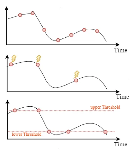
The figure 2.2 depicts values of a parameter over time and when events might occur based on different interaction patterns [2]. The upper curve has circular dots which represent the communication events spaced regularly by time delays scheduled in advance.
2.2 Event-based system Components
Figure 2.2: the Three communication patterns: scheduled-based, pull-based, and push-based
The middle curve has multiple pointing bolts represents the instance when external requests are triggered.
The lower curve has multiple circular dots which shows the time instances of when the values of the parameter value surpass given thresholds. So, events have been triggered accordingly.
Scheduled-based interaction requires synchronization between all the partic-ipants’ clock, otherwise it doesn’t work out effectively. Nevertheless, this kind of interaction does not suit scenarios where urgent reactions are needed because it makes restriction on the time slots available to transfer information(alerts).
On the other hand,Pull modeallows responders to initiate the interaction and ask for the current status observed by sensors. but when should Responders do so? Responders can’t predicate this failures time (i.e. failures could happen any time). Therefore, many communication rounds between components would be created even though there are
2 Literature Background
no useful information to share at the time of initiation. Moreover, This mode would consume much more resources.
This kind of interaction is useful when there are some limited periods, failures are more likely to happen (e.g. deployment of a new machine), but long term interaction, using this mode, costs high because of the frequent responses.
An alternate pattern is push information from sensors.The sensors implanted in
a production line or any other system might be organized in a hierarchical graph such as a tree. Each sensor sends messages when its measurements exceed a predefined thresh-old. Push technology requires precise shared models to determine what information to push [2].
Many systems combine advantages of poll and pull-based communication pat-terns by getting warning based on information pushed by sensors, and then acquisi-tion(request) of additional relevant information based on information pull [2].
2.3 Anomaly Detection Techniques
As the thesis concerns in detection of anomalies, we would like to conclude some common Machine Learning techniques which gives a wider sight over the field of anomaly detection.
2.3.1 Definition
Anomaly detection refers to the problem of finding patterns in data that do not conform to expected(normal) behavior [18].
Many challenges are implied within this definition as presented in [18] :
1. Defining the boundaries of every possible normal behavior is not an easy task. Especially, if we consider domains where normal behavior keeps evolving and the current definition might not be steady in the future.
2. Another issue is when anomalies are the result of malicious actions.These actions adapt themselves to be appeared as a normal or when data contains noise that tends to be similar to the actual anomalies.
3. Availability of labeled data which are needed to train and validate models used in anomaly detection. These models can be defined through long-run experience and might be alway tuned to reflect the normal/abnormal behavior. In our solution,
2.3 Anomaly Detection Techniques
the given probability threshold and number of transitions(N) to be considered serves this aspect.
2.3.2 Machine Learning Approaches to detect anomalies
Machine Learning techniques require an explicit or implicit model to establish. This model enables patterns under analyzing to be categorized into normal/abnormal. Apply-ing Machine LearnApply-ing(ML) principles intersect in many aspects with statistical techniques. However, ML includes building an adaptive model which improves performance and execution strategy depending on the previous results and any acquired information, but in the other side it consumes much more computation resources [17].
Bayesian Network
It is a probabilistic graphical model that represents a set of variables as nodes and their conditional dependencies as edges in a directed acyclic graph(DAG) 1. It is generally used in intrusion detection and sensor network along with statistical schemes to en-code interdependencies between variables and gives the probability of a future event occurrences[17].
Neural Network
It is a flexible approach and adaptive to environmental changes which enables creating behavioral profile and predicts a potential anomaly from a sequence of previous ones. It is applicable in domains such fault detection of mechanical units and performance monitoring of industrial components using sensor data [17].
This approach requires a training phase to build the neural connections properly based on variant normal classes provided as input data [18].
Rule-Based
Similar to neural network, Rule-based approach has two steps. the first step(training): is to learn rules from labeled data using rule learning algorithm such Decision tree.Thereby each rule is attached with confidence factor. The second step is to find the rule which captures the test instance[18].Thus, a test instance which is not covered by any of these
2 Literature Background
rules is considered as an anomaly. Rule-based technique covers multi-class and one basic class (e.g. association rule algorithm which generates rules in an unsupervised manner).
Clustering and Outlier detection
Clustering algorithms can be used to group data instances into clusters. According to similarity or proximity criteria(Euclidean or Mahalanobis distance), each new data point not classified to any cluster is considered as an anomaly. Furthermore, detection decision might be attached with certain degree of being an outlier[17].
3
|
Challenge Description
The focus of Grand Challenge 20171was on the analysis of RDF streaming data generated by digital and analogue sensors which embedded within manufacturing equipment. The ultimate goal of the challenge was to implement a solution which is capable of detecting abnormal behavior of hundreds of real manufacturing machines using stream of measurements provided by each machine. The Challenge consisted of two scenarios that relate to the problem of automatic detection of anomalies. The difference between the first and the second scenario is that in the first one the number of machines to observe is fixed, while in the second scenario new machines can dynamically join and leave the set of observable machines [16].
In addition to the correctness criteria which the solution should ensure, the per-formance and efficiency aspect takes an importance during the benchmark process. Therefore, the evaluation process was done using an online platform called Hobbit2 which provides automated test of the correctness, in addition it measures the throughput rate and the latency time of the solution.
In the following, we provide a description of the query that will be applied to detect anomalies in the behavior of the machines. Afterwards, we introduce the input and output data format.
3.1 Query Phases
DEBS Grand Challenge 2017(GC2017) addresses the problem of anomaly detection of machine behavior via Markov models technique. The intuition behind this technique usage is to model normal operations of a given machine. Then incoming event sequences
1This challenge is organized by Distributed Event-Based Systems(DEBS) conference 2Holistic Benchmarking of Big Linked Data: https://project-hobbit.eu/
3 Challenge Description
are compared continuously against models to determine the probability of their occur-rence. This mechanism considers event sequences as anomalies if they have - according to the model - a low probability of occurrence comparing to a probability of normal behavior [15].
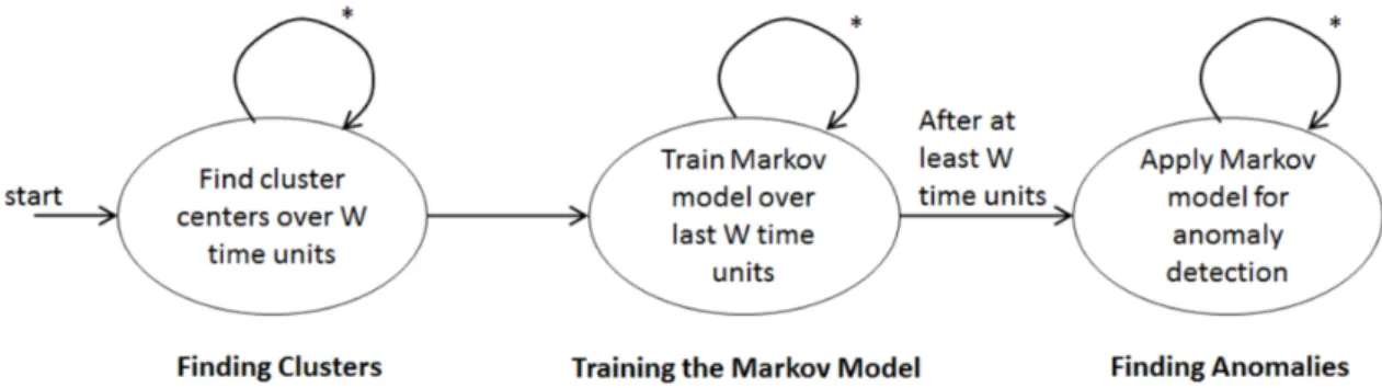
Overall, the anomaly detection comprises three steps which are depicted as [15]: (1) Finding Clusters using K-means algorithm.
(2) Training a Markov Model. (3) Finding Anomalies.
Finding clusters is a preprocessing step for mapping event values to discrete states. This is a prerequisite for training a Markov model in step two, that reflects transition probabilities between the observed states(clusters).
A requirement of the challenge is to execute the previous three stages only for events which falls under the last W time units. This is to account of incremental update of events and consider subset of incoming events in order to build Markov chain model. Step three uses the updated model to compute the probability of observing the last N received events. The mechanism reports an anomaly if the resulting value is below a given threshold [15].
Machine data have many sensors and the previous three steps must be executed for each sensor’s dimension separately.
Figure 3.1 provides an overview of the three described query steps as Nondeter-ministic finite automaton (NFA).
Figure 3.1:Three stages of the Grand Challenge Query - [16]
An event passes the sketched stages in sequence. Once the stream has started, the activities for each stage are executed continuously. This means, an incoming event (produced by each machine) makes a change on clusters that would be reflected on Markov model [16].
3.2 Data Description
It is important to notice that anomaly detection phase does not begin before receiving an adequate number of input values. In the challenge’s context, we refer to the required input set to start executing the query as window size which defines the time period between the first and the last event. Thus, several internal buffers are used to maintain historical events data until the window becomes full; only then, the subsequent phases can be triggered.
In Chapter [5], we introduce variant types of window policies used in event-based systems and provide our implementation details upon it.
3.2 Data Description
The input data has two parts: (1) metadata and (2) measurements. Both are represented in RDF and formatted using N-triples. Basically RDF is simple and well expressive data model. The primitive unit of information is defined as a triple (Subject, Predicate, Object). N-Triples triples are separated by white space or tabs. Each sequence of its components is terminated by a ’.’ and a new line. [6].
3.2.1 Metadata
Metadata is given as a static file which includes information about the machine type, the number of sensors per machine, max number of clusters that must be used in order to detect anomalies during K-means stage and a probability threshold which the multiplicative probability of last N-sequence should be compared with during anomaly detection stage.
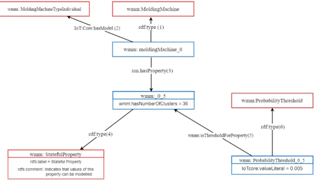
Below is a sample of RDF Metadata which provides information about one machine (machine_0) and one of its dimensions (dimension_5). Associations in figure 3.2 are defined by predicate component of each triple. These associations are enumerated in the figure to ease tracking the following triples.
Machine_IDis unique through all Metadata file. Machine_0object is derived from class MoldingMachinevia Link(1).
wmm:Machine_0 rdf:type wmm:MoldingMachine .
wmm:Machine_0 IoTCore:hasModel wmm:MoldingMachineTypeIndividual .link(2)
dimension_0_5of the molding machine is depicted through link(3).
3 Challenge Description
Property _0_5has a numerical value. Thus, it is linked to wmm:statefulProperty node via link(4).
wmm:_0_5 rdf:type wmm:StatefulProperty .
Number of clusters is a property indimension_0_5 node.
wmm:_0_5 wmm:hasNumberOfClusters "36"8sd:int .
There is a threshold for each dimension. It can be obtained via link(5).
wmm:ProbabilityThreshold_0_5 wmm:isThresholdForProperty wmm:_0_5 .
ValueLiteralis a property inwmm:ProbabilityThreshold_0_5node.
wmm:ProbabilityThreshold_0_5 IoTCore:valueLiteral "0.005"8sd:double> .
ProbabilityThreshold_0_5is an object derived fromwmm:ProbabilityThresholdtype via link(6).
wmm:ProbabilityThreshold_0_5 rdf:type wmm:ProbabilityThreshold .
Figure 3.2: MetaData structure. Red rectangles represent user-defined classes whereas blue ones represent object instances.
3.2.2 Observation Groups (Events)
Injection molding machines are equipped with sensors that measure various parameters of a production process: distance, pressure, time, frequency, volume, temperature, time, speed and force.
3.2 Data Description
Each machine produces at a particular timestamp oneObservationGroup(event) which constitutes of 120 dimensional vector. These dimension’s values are, in principle, sensor readings which are given in different types either textual (string) or numerical (integer or double). All measurements are provided as RDF triples or more precisely as instances of an OWL ontology which is available via HOBBIT CKAN site3[16].
For the challenge purpose, we only deal with dimensions which hold numerical values(stateful properties), since they are only applicable for K-means clustering phase. Therefore, receiving any textual value should be filtered for the subsequent phases during stream processing.
Each Observation Group has a timestamp which refers to the time when the event has been produced by the machine. However for the sake of the challenge, the generation of events stream by evaluation platform does not necessarily reflect timestamp differences between subsequent events. Which means, higher throughput speed might be applied irrespectively of the timestamp’s values that ObservationGroups hold.
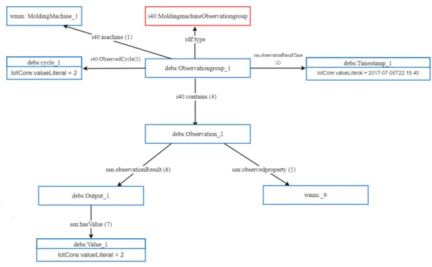
Below is an example of N-Triples format forObservationGroup_1. Obviously, Each observation group has a unique identifier that associates with a particularMachine_ID (link 1) that is bound, in turn, with machine information provided already in metadata.
In addtion Each observation group has a timestamp(link 2), cycle (link 3) and many Observations.
debs:ObservationGroup_1 rdf:type i40:MoldingMachineObservationGroup. debs:ObservationGroup_1 ssn:observationResultTime debs:Timestamp_1. debs:ObservationGroup_1 i40:contains debs:Observation_2.
debs:ObservationGroup_1 i40:observedCycle debs:Cycle_1. debs:ObservationGroup_1 i40:machine wmm:MoldingMachine_1.
Injection cycle value is a property of Cycle type.
debs:Cycle_2 rdf:type i40:Cycle.
debs:Cycle_2 IoTCore:valueLiteral "2"xsd:int.
debs:Timestamp_1 rdf:type IoTCore:Timestamp.
debs:Timestamp_1 IoTCore:valueLiteral "2016-07-18T23:59:58"xsd:dateTime.
Here we include only Observation_2 via link(4) which is an object of
i40:MoldingMachineObservation type. It is connected via link (5) to dimension_9
and via link(6) to output_1
debs:Observation_2 rdf:type i40:MoldingMachineObservation.
3 Challenge Description
debs:Observation_2 ssn:observedProperty wmm:_9.
debs:Observation_2 ssn:observationResult debs:Output_1.
Output_1 is an object of ssn:SensorOutput type4. it is connected via link (7) to Value_1.
debs:Output_1 rdf:type ssn:SensorOutput. debs:Output_1 ssn:hasValue debs:Value_1.
Value_1 is an object of i40:NumberValue type which has the actual value as a property.
debs:Value_1 rdf:type i40:NumberValue.
debs:Value_1 IoTCore:valueLiteral "-0.01"xsd:float.
Figure 3.3 depicts associations structure between the previous triples.
Figure 3.3: Events Data structure
As we can notice the actual sensors’ values can be obtained by traversing the graph through this property path:
i40:contains/ssn:observationResult/ssn:hasValue/IoTCore:valueLiteral.
4SSN (semantic sensor network) an ontology derived from the OWL describes sensors and observations,
3.2 Data Description
3.2.3 Output
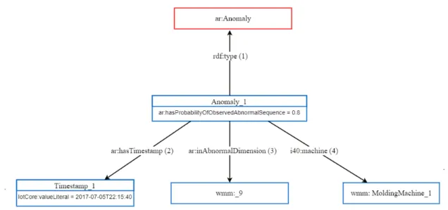
The output provides information about any detected anomalies. Anomaly Output contains a unique ID generated by the system, sensor(dimension)_ID and Machine_ID whose the anomaly belong to. In addition, it includes timestamp of the Observation group which is located at the beginning of anomaly sequence(see 5.4.3).
The output data stream should be ordered based on the timestamp which Observa-tionGroup has. Moreover, if one observation group produces many anomalies, then the output data are sorted in ascending order based on thedimension_ID.
The figure3.4 depicts output structure and the following N-triples is a serialization format.
UserNamespace:Anomaly_1 rdf:type ar:Anomaly. link1
UserNamespace:Anomaly_1 ar:hasProbabilityOfObservedAbnormalSequence "0.8"8sd:float.
Anomaly_1is connected withdebs:Timestamp_4via link (2).
UserNamespace:Anomaly_1 ar:hasTimestamp debs:Timestamp_1. UserNamespace:Timestamp_1 rdf:type IoTCore:Timestamp.
UserNamespace:Timestamp_1 IoTCore:valueLiteral "2017-01-17T00:15:00".
UserNamespace:Anomaly_1 ar:inAbnormalDimension wmm:_9. link3
UserNamespace:Anomaly_1 i40:machine wmm:MoldingMachine_1. link4
3 Challenge Description
Query Parameters
There are several parameters used through execution’s phases of anomaly detection [16], These parameters are:
N: number of transitions to be used for combined state transition probability. M: number of maximum iterations for the clustering algorithm.
Td: the maximum probability for a sequence of N transitions to be considered an anomaly. The value of Td is specified for each dimension d for which the clustering is performed. This value is read from Meta data.
W: window size for finding cluster centers with k-means clustering and for training transition probabilities in Markov model.
Applying different parameters values affects significantly on the executions perfor-mance as well as the results accuracy. As an example, having a big value of M (number of iterations) might yield to a long execution time. But on the other side, it makes the points assignments more precise.
4
|
System Design
The system is designed to fulfill the challenge’s requirements explained in the previous chapter. The system is built using C#.net (version 4.5) under Visual studio IDE. Basically the execution takes place in the background, with a possibility to adapt the parameters’ values interactively.
The program is able to receive events stream either from a message bus service (e.g. RabbitMQ) or directly from a local RDF file. As well as the possibility to interact with Hobbit platform using a special adapter 1. The solution reacts based on event receiving (Push-based interaction) on its input queue.´This means, the system is idle until it receives any valid message (see [6.1]), upon then it processes the message’s content. In case an anomaly is detected, a message is sent to the platform using an output queue (further details are given in chapter [6])).
4.1 System Components
The execution core of the solution comprises of 6 main components which are categorized here based on the section’s purpose. Thus, the section might be part of a class (methods) or several classes. These sections are:
1. The Coordinator. 2. System Adapter. 3. Metadata Reader. 4. Observations Reader. 5. Event Distributer.
1The platform is provided by Challenge organizers as a mean to benchmark participants’ solutions
4 System Design
6. Pipeline phases (a) Sliding Window. (b) K-means.
(c) Markov Model building. (d) Anomaly Detection.
We introduce here briefly the purpose of each component.
The Coordinator: assigns parameter values, initiates objects of System Adapter, Metadata Reader.
System Adapter: This singleton component works as a communication moderator between the benchmarked system and the evaluation platform. It interacts with Hobbit platform through three channels (queues), mainly to receive commands and stream data and to send the output results.
However, before start receiving any events (Observations stream) some coordination messages must be exchanged. More details about Hobbit platform API and how our system adapter comply with will be elaborated in Chapter 6.
Metadata reader: has the task of reading Metadata file which is included as an embed-ded resource within the system. Mainly the object has to extract only the necessary information and maintain them in a designed data structure to aim of further processing. The resource is provided in advance internally since the evaluation platform sends only observations events.
Observations Reader: receives the Observation Group, as one event, from the system adapter. Each observation group describes sensors readings of a machine at a specific time. The reader splits each observation Group into its containing triples to extract and maintain what it is relevant to the challenge context(further details see 5). Event Distributer: each dimension (property) of each machine has its own pipeline path used to execute the main three phases (window shifting, k-means, Markov model, Anomaly detection).
Thus, distributing the work occurs whenever reading of one observation group is finished in order to forward the event’s data over the appropriate pipeline’s path. Moreover, variant approaches to parallelize the execution (e.g. threads) takes place here (further details in section4.3).
4.2 UML Diagrams of the system
Pipeline phases: is held concurrently for each dimension of each machine. This means, in case of an event consists of 55 stateful dimensions, this would lead to 55 pipeline paths to work either in a parallel or in a sequence.
Unlike the previous singleton objects which work on all incoming data, here k-means and Markov-model objects are fully dedicated to only one dimension’s data. (a) Sliding Window: newly received value must be added into the window. It Shifts
the window respectively(If needed) and drops the earliest event (further details in chapter 5).
(b) K-means: once we have an adequate number of data points within the window, K-means is applied on the respective dimension. Some requirements has been set on K-means implementation by organizers will be introduced in chapter [5]. (c) Markov Model building: used to maintain the transactions history between clusters’
centers resulted in from K-means phase. As well to produce the probability’s array of movement between any state to any other.
(d) Anomaly detection: calculates the multiplicative probability of transitions for the last N states using probability array from the previous phase. Then the result is compared with a special threshold maintained for this dimension.
If an anomaly is detected, this would trigger an alert immediately and would attach all the anomaly’s information.
The output should be provided as bytes (UTF-8 encoding) and sent to System Adapter again which held the responsibility of forwarding the results to Hobbit platform.
4.2 UML Diagrams of the system
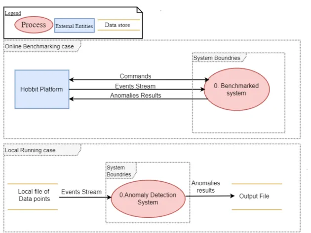
4.2.1 Context Diagram
Figure 4.1 depicts the context diagram of the system which is represented as a single high-level process. In addition, it shows input/output messages exchanged between the system and other external entities (Hobbit platform, external data stores, etc.).
4 System Design
Figure 4.1:Context Diagram-Level-0
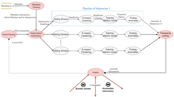
Figure [4.2] depicts data flow diagram of process 0 (Benchmarked System) from context diagram figure. Figure [4.2] shows how data flow between sub-processes and memories. Here we replicated pipeline processes to indicate that we have similar behavior for each dimension data. The number of replications equals to the number of stateful dimensions in the corresponding machine.
4.2 UML Diagrams of the system
Figure 4.2:Data Flow Diagram of process 0.Benchmarked System
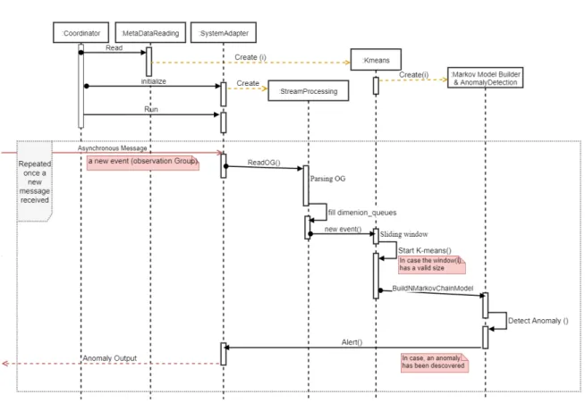
4.2.2 Sequence Diagram
Figure 4.3 provides the sequence diagram which depicts clearly the overall interactions among those divisions over time. Note that red arrows indicates to messages from/to outside the boundary of the solution.
Also the big rectangle encircles the respond part of the event-based system since the solution listens always to its external queues and reacts upon it.
Create(i) messages: indicate to the initiation’s calls of pipelines objects for all dimensions(properties) of all machines.
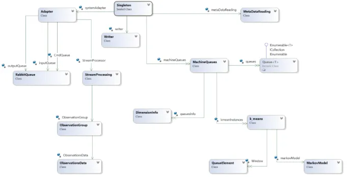
4.2.3 Class Diagram
Figure 4.4 depicts the class diagram of our system which describes the structure of the system (i.e. the classes and the relationships among them)
Note thatSingletonis static class that contributes in initiating several unique (only one) objects such systemAdapter, MetaDataReading and one List of MachineQueues.
4 System Design
Figure 4.3: UML:Sequence Diagram of the system
EachMachineQueueselement maintains, in its turn, list of several queues (one for each dimension).
Also K-means objects are connected to those queues through the list of Ma-chineQueues becasue each object of k-means algorithm is specialized to work on one dimension and not intervene with other dimensions data. Furthermore, MarkovModel object is created along with the creation of its related k-means object (one to one relationship).
4.3 Distribution Possibilities
Although there are multiple potentials to parallelize the tasks within the solution in order to elevate the performance and decrease the overall latency, but in the other hand, there are some dependency constrains set by requirements which limit the advantages of having a distributed version.
4.3 Distribution Possibilities
Figure 4.4:Class Diagram of the system I would like to enlighten here some of those constrains:
First constraint: The anomalies output(if there any) should be sorted based on the same time order which the input events were pushed.
Therefore, in case we want to distribute events over multiple nodes or threads. This would require a synchronization in outputting the anomalies to respect the same order.
In other terms:
Two subsequent events: et < et+1 if event etcauses Anomalyi
if event et+1 causesAnomalyj
then outputAnomalyi beforeAnomalyj
Second constraint: In case we detect more than one anomaly within the same observa-tion group, then these anomalies should be sorted based on the dimension ID order. In other terms:
Event etcauses Anomalyi
Event etcauses Anomalyj also
if (dimension[Anomalyi] < dimension[Anomalyj])
then Alert(Anomalyi) before (Anomalyj)
To tackle those issues and make the solution distributed as possible, we focused on the system’s sections which might benefit from having multiple threads. Here we propose various approaches to enable distribution option.
4 System Design
First of all, we would like to clarify some expressions which we will use to avoid misunderstanding.
Event preparing: refers to all the steps needed before pipeline execution. This includes receiving the events from the platform, reading the content, splitting the work over corresponding dimensions and triggers the respective pipeline.
Pipeline execution: refers to a complete execution of all phases starting from K-means building Markov-Model and then anomaly detector for all dimensions of one observation group.
First option:
To avoid having a synchronization issue which might be caused by the second constrain. One might choose a simple but effective scenario by choosing one thread fully dedicated to events preparing and another thread for pipeline execution.
Once event preparing is over, the second gets active. In meanwhile of pipeline executions, if a new event has been received from the platform, it will be prepared immediately.
Figure 4.5:One thread for preparation, one thread for pipelines’ execution
Second option:
Empirically, The time taken for event preparing is relatively small comparing to the execution time of all relevant pipelines (i.e. especially if the window size is relatively
4.3 Distribution Possibilities
large).
Tpreparing << Tpipelineexecution
In this context, it is better to assign a fixed number of threads to take control of the pipeline executions. which means, each thread executes several dimensions’ pipeline. But eventually all threads need to wait until the other threads dimension output to finish (to respect the second condition).
However, detecting whether other threads have finished their pipeline’s exe-cution (in sake of correctly order the anomalies) is not also an easy task, since it requires a periodically check. In meanwhile of pipeline executions, a new event can be prepared by the specialized thread. The following figure [4.6] shows this scenario
Figure 4.6:One thread for preparation, multiple threads for pipelines’ execution If we assumed that event preparing consumes much time than the pipeline executions (i.e. a small window size or small value of M). Then assigning more than one thread for reading a single observation group might accelerate the overall execution time. Hence, ensuring that reading part does not make any bottleneck.
4 System Design
Third option:
Up now we have only scaled up, however scaling out means adding more ma-chines(nodes) to run the same process (event preparing + pipeline execution). The hardest part then would be to split and synchronize properly.
One splitting criteria is distribute the incoming events over machines in a fair scheme and apply one of the previous options internally. By doing so, collection all of anomalies from all machines into one location need to be done, to make sure the order of the events is respected (the first constrain).
This synchronization operation might lead to an extra pay-off, if one machine takes accidentally long time to output its event (its event precedes the others) or if the communication channels suffers from latency.
As a conclusion, there is no 100% correct option to apply which ensures effectiveness in all aspects (high performance, low latency, valid for all window sizes and respect constrains). Therefore, we have run several tests for multiple scenarios using different parameter’s values (e.g. W,M).
5
|
System Implementation
5.1 RDF Processing
5.1.1 RDF Stream Parsing
The system should parse RDF content and extract the necessary information in an efficient and fast manner to reduce the overall latency and achieve high performance results. Each event is a single observation Group(OG) which follows the data scheme explained in Challenge Description Chapter. OG contains approximately 950 triples encoded as UTF-8 bytes.The steps to parse streaming RDF are:
1. Convert bytes to string type, split each OG into its containing triples by using period(.) as a splitting character.
2. Split each triple into its components (S,P,O) by using (white space) as a splitting character.
3. Make comparisons between string constants and all triples’ predicates resulted in from previous step. Such comparisons is achieved usingSwitch Casestatements. Hence, immediate discard of the triples which are not relevant for further process-ing while maintainprocess-ing object/subject values of necessary triples.
In the following, we drew lines under those predicates whose subject/object’s values are interesting, therefore they would be maintained.
First partof an OG is the header which consists of triples to define OG_ID,Timestamp, Cycle and Machine_ID:
debs:ObservationGroup_1 rdf:type i40:MoldingMachineObservationGroup. debs:ObservationGroup_1 ssn:observationResultTime debs:Timestamp_1. debs:Timestamp_1 rdf:type IoTCore:Timestamp.
debs:Timestamp_1 IoTCore:valueLiteral "2016-07-18T23:59:58"xsd:dateTime. debs:ObservationGroup_1 i40:observedCycle debs:Cycle_1.
5 System Implementation
debs:Cycle_2 rdf:type i40:Cycle.
debs:Cycle_2 IoTCore:valueLiteral "2"xsd:int.
debs:ObservationGroup_1 i40:machine wmm:MoldingMachine_1.
Second Part is for observations definition (here we provide only one) which con-tains triples of Dimension_ID, Observation_ID, Output_ID and Value_ID:
debs:ObservationGroup_1 i40:contains debs:Observation_2. debs:Observation_2 rdf:type i40:MoldingMachineObservation. debs:Observation_2 ssn:observedProperty wmm:_9.
debs:Observation_2 ssn:observationResult debs:Output_2. debs:Output_2 rdf:type ssn:SensorOutput.
debs:Output_2 ssn:hasValue debs:Value_2. debs:Value_2 rdf:type i40:NumberValue.
debs:Value_2 IoTCore:valueLiteral "-0.01"xsd:float.
For each observation, we are ultimately interested in the float value(the object node of IoTCore:valueLiteral predicate), although, we still maintain Observation_ID, Output_IDandValue_ID. This because we need to keep the reference of each value to its related Observation_IDand hence its related dimension. Especially, in cases where these IDs are not all equal (e.g. Observation_1, Output_3, Value_5) then it would not be feasible to determine which value belongs to which dimension.
Figure 5.1 shows ObservationGroupand ObservationsData classes in the system whose their attributes should be filled while reading a single event(OG).Both classes are initiated once. However, they are initialized each time a new event is received after moving their content to another data structure(see 5.2). In other words, these classes’ objects serve as a data container of incoming events to match the event data with corresponding information from metadata.
5.1 RDF Processing
5.1.2 Metadata Parsing
Metadata are provided as a file embedded within the system. The file has string type(i.e. no need for type conversion). Each triple comes typically in one line(i.e. no need for triples separation). Using StreamReaderclass provided by C#, one can iterate over the file to filter unnecessary triples and keep object/Subject values which belong to specific predicates.
In he following, we provide one machine definition, interesting predicates are under-lined:
wmm:Machine_0 rdf:type wmm:MoldingMachine .
wmm:Machine_0 IoTCore:hasModel wmm:MoldingMachineTypeIndividual . wmm:MachineModel_0 ssn:hasProperty wmm:_0_5 .
wmm:_0_5 rdf:type wmm:StatefulProperty .
wmm:_0_5 wmm:hasNumberOfClusters "36"8sd:int .
wmm:ProbabilityThreshold_0_5 wmm:isThresholdForProperty wmm:_0_5 . wmm:ProbabilityThreshold_0_5 IoTCore:valueLiteral "0.005"8sd:double> . wmm:ProbabilityThreshold_0_5 rdf:type wmm:ProbabilityThreshold .
For each machine definition given in metadata file, we initiate a new object of each class shown in figure 5.2. Moreover, red-colored attributes are filled during Metadata parsing. MachineQueuescontains number of internal queues equal to the number of the machine’s dimensions.
In the other hand,QueueElementdefines element’s type of the queue. it has sensor reading taken from ObservationsDataobject (presented above). whenMachine_IDare identical.
5.1.3 Pros and Cons of our approach
Advantages:1. No need to allocate extra memory for representing event’s triples in a graph which is the basis of common RDF processing libraries (e.g. DotNetRDF1).
2. Provides a high-performance and customized approach to parse RDF data and extract information out.
3. Discard unnecessary, keep the relevant information: this approach fits well with streaming fashion; Once we extract information from a triple we don’t parse it
5 System Implementation
Figure 5.2:MachineQueues class and its associations
later; whereas RDF libraries builds triples graph and then start traversing the desired value through edges and nodes of the graph.
4. Support arbitrary order of triples, this means no need to have a pre-defined order of triples within each event.
Disadvantages:
1. It requires a high number of string comparisons and string trims to extract the desired information out.
2. It is not generic approach: It needs to be re-customized in case of any change regarding data scheme or RDF serialization.
5.2 Sliding Window
Pipeline phases ae not applied on individual event, but on subset of streaming events. This subset is denoted asSliding Windowand it is updated continuously based on variant policies. We would like to give, in this part, a quick overview of those policies and then
5.2 Sliding Window
dive in details with our approach properties and how it was realized for the sake of challenge scenario.
5.2.1 Eviction and Trigger Policies
The sliding window has two policies of update: anEviction policyand a Trigger pol-icy.The eviction policy defines when window’s event should be excluded out. Sliding window drops only those events which are expired, Unlike tumbling kind of window where the whole window is emptied and refilled from scratch. In the other side, Trigger policy defines the criteria of inserting new events into the window [7].
There are three types of eviction/triggering policy for sliding window explained : 1. Count eviction policy: this policy allows the sliding window to maintain up to N
events then it is considered full [7]. Any new arriving event would enforce the oldest event to be expelled out; except of that existing N events stay in the window for forever.As an example, Count(5)specifies 5 events as a maximum size of data to maintain.
Count trigger policy: states that the sliding window is triggered for every new N tuples that arrive [7]. In another term, these events would wait outside the window until they become N events, only then they trigger a sliding action. For instance, Count(1)triggers the window for each new input event.
2. Time eviction policy: An event must be evicted, if it has been in the window for more than T time units [7]. As an example, Time(10 seconds) policy would let events stay within the window for 10 seconds. This means the window would always contain the last 10 sec events. This kind of policy is expensive and requires a continuous monitoring to ensure the window’s correctness since time is always increasing and can be seen as a permanent trigger.
Time trigger policy: time(T) states ’that the sliding window is triggered every T seconds, regardless of event arrival’ [7].
3. Delta eviction policy: this policy has two parameters: attributeto evaluate a condition based on its values and atime delta value. In the other words, when a new event e arrives, we compare its attribute’s value with those in the window. If the difference is larger than Threshold, then we expelled the event out of the window we express this condition as follows [7]:
5 System Implementation
If the attribute to consider has always an increasing value (e.g. timestamp )the previous condition is valid. However, if an incoming event holds an attribute’s value smaller than any value in the window, this would make the condition always satisfied irrespectively of the threshold. Therefore, we update the condition, as follows:
|valueincoming_event−valueevents_of_window|>=T hreshold
Delta trigger policy: When an event earrives at the window, the difference for attribute is calculated between (e) and the last event that triggered the window [7]. If the difference fulfills the condition, the window is triggered. For example Delta(ts, 3), where ts is a timestamp attribute, the window will be triggered every 3 seconds according to timestamps of the data.
To ease the comparison for this policy type, It is recommended to keep the events in the window sorted according to the attribute values.
One should keep in mind that these policies can be applied as eviction or triggering in an independent way and in any combination.
5.2.2 Implementation Details
In the context of the challenge, the system responds to each and every incoming event and pushes relevant event’s data into the window. This means the system should apply count trigger policycount(1).
In the other side, the window includes events whose timestamps belong to the lastW time units. Therefore, we have to compare the new incoming event’s timestamp with the window event’s timestamp. if the difference is larger than W, we evict the related events out of the window. This means the system should apply a Delta eviction policy Delta(Timestamp,W).
In general,time eviction policycan do the same work as Delta eviction policy e.g. Time(W), if the attribute is an increasing timestamp. However, the time intervals of streaming events do not reflect the real timestamps difference. therefore we can’t rely on time as an eviction criterium for the challenge’s purpose. Moreover, applying time eviction is much more expensive.
Figure 5.3 shows sliding window example that clarifies eviction and trigger policies followed in our system.
5.3 Clustering using K-means
Figure 5.3:Sliding Window example
5.3 Clustering using K-means
5.3.1 General description
K-Means is one of the most popular "clustering" algorithms. The input of the algorithm is set of numerical data that composed of number of dimensions >= 1.
No labels are given to the algorithm since it is unsupervised kind. Labels are an essential ingredient for supervised algorithms which have predefined categories[14].
The output of the algorithm is groups of data called clusters. These clusters contain points which are closer to the center of the cluster, whose they belong, than any other cluster.
K-Means finds the best centroids by alternating between [14]: (1) assigning data points to clusters depending on the distance.
(2) calculating cluster centers (centroids) based on the assignment of data points occurred in the first phase.
5 System Implementation
The purpose of clustering within the Challenge scenario: As we have many data points in each window, modeling all distinct values directly using Markov chain would not be effective. Therefore, we group all the datapoints whose their value are close to each other under one cluster. This helps representing each cluster(set of values) as one single state later in Markov model chain.
5.3.2 Clustering in the context of the Challenge
We are given a training setx1,...,xw (w: size of the window). We want to group data into a few cohesive "clusters." Each Datapoint represents one sensor reading. Hence, it forms one dimensional numerical dataxi ∈
R; but without labelsyi. Our goal is to label each datapoint within a cluster ci.
GC’s Special Requirements
K-means must be applied on each dimension of each individual machine. This implies having hundreds of k-means instances and enables designing a parallel/distributed approach since there is no information intersection between these instances.
In order to make the results of the algorithm deterministic and make the correctness evaluation more accurate, many requirements were given by organizers to clear the ambiguity of special cases such:
1. Each Dimension of each machine has its own value of (K) which is taken form Metadata file. K represents the number of clusters in the normal case (The special case see req.3).
2. To determine the initial cluster centers(centroids) after sliding the window, we use the first K distinct values, in the stream of that dimension, as seeds.
3. If a given window contains less than K distinct values. Then the number of clusters would be equal to the number of distinct values that we received so far. Nevertheless, in the following iterations, we use all events within last W time units to find the final cluster centers.
4. If a data point has the exact same distance to more than one cluster center, it must be associated with the cluster that has the highest center value.
k-means execution comes to an end when one of the following criteria fulfills: (a) Iteration counter reaches a given parameter(M: Maximal number of iterations). (b) Convergence condition: All centroids’ values of two subsequent iterations get equal.
5.3 Clustering using K-means
To specify the equivalence accuracy,especially that values are float. We take on Cluster precision (P) parameter: which determines if the distance between an old centroid and a new candidate is considered equal or not. Thus, if the distance was less or equal the clustering precision, we don’t take into account the new candidate as a distinct centroid.
5.3.3 Implementation
The main procedure of K-means algorithm is provided below [K-means algo.] as pseudo-code.
Algorithmus 5.1K-means algorithm Input: set of data points (DPs). Output: K Clusters. Begin: 1. InitialAssigningofClusterCenters(); do { 2. iteration := iteration + 1; 3. DatapointsAssigning(DPs); 4. UpdateCentroid(); }
5. while (not K-meansFininshed());
6. BuildMarkovChain(DPs,Number of Cluster(K), DataPointCluster); End.
All other methods which are called by this procedure are attached within appendix section[Appendix B] at the end of the thesis such:
1. InitialAssigningOfClusterCenters: is called at the beginning of K-means execution in order to assign the initial centroids(seeds).
2. UpdateCentroid: calculates the centroids’ location once each iteration.
3. DatapointsAssigning: iterates through datapoints of the window and assigns each point to the cluster whose its centroid location is the nearest.
4. K-meansFininshed: checks if any termination’s condition is met at the end of each iteration. Based on, it returns a boolean decision.
5 System Implementation
5.3.4 Proposed optimization : Confined Influence
we propose an improvement for k-means algorithm specified for one-dimensional data. By applying this optimization, we consider only the points of clusters which are directly adjacent to updated clusters in the previous iteration, rather than checking all point’s distance to all clusters in each iteration (classical k-means algorithm). The principle is to measure the influence of the updated clusters on their neighbors, before propagating and calculate distances for farther points. Thus, we make sure that the effect is confined only to neighbors.
Next we provide next pseudo-code of k-means which includes the proposed optimization.
Algorithmus 5.2K-means algorithm including the optimization Input: set of data points (DPs).
Output: K Clusters. Begin:
1. Repeat until convergence {
2. Labelci whereci clusters that had a change in the last iteration.
3. For each datapointxawhich belongs to clusterca(adjacent toci)
4. if|xa−ua|>|xa−uj|//uj anduacentroid ofci, caaccordingly
5. Assignxatoc i
6. Update Centroids }
End.
Therefore, In each iteration, we label the clusters that had a change in cluster center’s location in the previous round (i.e. points are added or deleted to/from this cluster). We consideronlydatapoints which are directly adjacent to the labeled clusters. We calculate the distance of these datapoints to the labeled neighbor. If the absolute distance of any datapoint is less than its current distance, we allocate the point to the marked cluster. This optimization requires having an ordered list of cluster centers at the first iteration, so we can indicate neighbors easily by list index.
Figure [5.4] shows six clusters, only two clusters(4 and 5) are updated in the last iteration(i-1), therefore they are labeled. In the current iteration(i), datapoints of 3,4,5 and 6 clusters (the neighbors of marked clusters) need to be reconsidered. But farther points(those belong to cluster 1 and 2) are not affected. Therefore, their datapoints don’t get touched.
5.4 Anomalies detection
Figure 5.4:Clusters of one dimensional data, clusters 4,5 are labeled
5.4 Anomalies detection
5.4.1 Types of Anomaly
Anomalies can be categorized into three types based on their nature [18]:
1. Point Anomalies: if an individual data instance is considered as an anomaly always compared to the rest of data. For instance, a product weights more than the normal standard weight. it can be immediately detected.
2. Contextual Anomalies:if an individual data instance is considered anomaly in a specific context(situation), but outside this context it might represent a normal case. The context is affected by the nature of the data set which imposes two attributes:
(a) Contextual attributes: are used to determine the context itself. For instance, in time series data, time forms a contextual attribute to determine the position of the data instance comparing to its neighbors (the entire sequence).
(b) Behavioral Attributes: are used to determine non-contextual aspects of an instance. An example, minus zero temperature is normal during the winter, but considered outliers during the summer.
The anomalous behavior is detected based on the values of behavioral attribute but within the contextual attribute.
3. Collective anomalies:if acollectionof data instance is anomalous with respect to the entire data set. As an example, if a sequence(collection) of sensor readings causes an anomaly within a window.
Nevertheless, A point or a collective anomaly can be a contextual anomaly if it is analyzed based on its context.
5 System Implementation
Output of Anomaly Detection
the output results could be typically either as ScoresorLabelsbased on the algorithm and data nature[18]. Scores: a score is attached to each data instance to refer to its degree of being anomaly. Based on score order, one might select subset of anomalies which are listed at the top. Labels: a binary categorization in which data instance is labeled as anomaly or not.
Based on the previous concepts, we can categorize anomalies,in the context of Grand Challenge, undercollective type because we consider the last N transitions within a window that covers W time units. In addition they arecontextual because anomalies are attributed with a temporal context and they have Behavioral Attributes (sensor values). In the other side we output anomalies when a transitive probability is below a predefined threshold, otherwise we consider the data sequence normal(e.g. Labels type).
5.4.2 Anomaly detection in the challenge: Markov Model
Markov chain is built out from a sequence of directed edges between nodes (states) These edges are associated with a probability calculated based on the historical transitions between a source and a destination node. As soon as we determine all the states of Markov Chain Model, we can start interpret the sequence of events into transitive probabilities along edges.
Typically, the normal behavior would be more frequent to happen than the abnormal one. This means a high transitive probability over the edges between the frequent states. Whereas the abnormal behavior would be associated with a low probability (relatively).
In the context of Grand Challenge, nodes of Markov Chain model are the clusters(from K-means phase) that contain similar sensor readings. Sequence of values which are rare to occur within a time window would imply to a defect in machine behavior. Thus, an alert should be outputted.
Once time window is shifted, new Markov model is rebuilt since clusters(nodes) would be different and accordingly transitions must reflect the new event sequence.
5.4 Anomalies detection
Markov Model : Mathematical Aspect
A stationary Markov chain is a special type of discrete time stochastic process2. It is a sequence of random variables X1,X2„X3„ ... having theMarkov propertywhich sates that the probability of moving to the next state at t+ 1depends only on the present state at tand not on the previous states leading to the state at timet[8].
the probabilities which label the edges of Markov chains can be represented asTransition Probability Matrix(a square matrix of size k) If the system has a finite number of states, 1, 2, . . . ,K [13]. P = P11 P12 ... P1k P21 P22 ... P2k ... ..