Portfolio Optimization with PCC-GARCH-CVaR model

Portfolio Optimization with PCC-GARCH-CVaR

model

Master’s Thesis in Statistics

Financial Theory and Insurance Mathematics

June 2 2014

Linda Mon Xi

UNIVERSITY OF BERGEN

Abstract

This thesis investigates the Conditional Value-at-Risk (CVaR) portfolio optimization ap-proach combined with a univariate GARCH model and pair-copula constructions (PCC) to determine the optimal asset allocation for a portfolio.

The methodology focuses on minimizing CVaR as the risk measure in replacement of vari-ance used in the traditional optimization framework of Markowitz. GARCH model provides a tool for predicting and analyzing the time-varying volatility financial assets are exposed to, while copulas allow us to model the non-linear dependence structure and margins separately. We compare the performance of the CVaR optimized portfolio with other investment strategies such as Constant-Mix and Buy-and-Hold. Although the selection of strategy de-pends on the investor risk profile, it is empirically shown that the proposed CVaR optimized portfolio outperforms the other two investment strategies based on the accumulated wealth in the long run.

Acknowledgements

First and foremost, I would like to thank Prof. Kjersti Aas, for her great guidance on finding the topic and excellent supervision during the writing of this thesis.

Furthermore, I would also like to express my gratitude to both my fellow Master’s Degree students for interesting discussions during lunch breaks, and the faculty members and staff at the Department of Mathematics, for making the study period enjoyable and smooth.

Finally, I would like to thank family and friends for their moral support and words of encouragement throughout the study period.

Contents

Abstract i

Acknowledgements iii

List of Figures vii

List of Tables x 1 Introduction 1 2 Portfolio Optimization 5 2.1 Risk Concepts. . . 6 2.2 Risk Measures . . . 7 2.2.1 Conditional Value-at-Risk . . . 8 2.3 Efficient frontier . . . 10

2.4 Mean-CVaR Portfolio Optimization. . . 11

2.5 Compared to Mean-Variance Portfolio Optimization . . . 12

3 GARCH 13 3.1 Volatility . . . 13

3.2 GARCH process . . . 15

3.2.1 GARCH(1,1) . . . 16

3.3 Non-Gaussian Error Distributions. . . 17

3.3.1 Generalized Error Distribution . . . 18

3.3.2 Student’s t-distribution . . . 18

3.3.3 Skew Student’s t-distribution . . . 19

3.4 Parameter Estimation . . . 19

3.5 Simulation. . . 20 v

vi CONTENTS 4 Copulas 21 4.1 Definition . . . 22 4.2 Elliptical copulas . . . 23 4.2.1 Gaussian copula . . . 23 4.2.2 Student’s t-copula . . . 24 4.3 Archimedean copulas . . . 25 4.3.1 Clayton copula . . . 26 4.3.2 Gumbel copula . . . 27 4.4 Dependence measures . . . 28 4.4.1 Concordance . . . 29 4.4.2 Tail dependence . . . 30 5 Vine-Copula 33 5.1 Pair-Copula Constructions. . . 34 5.2 Regular Vines . . . 35 5.2.1 C-vine . . . 36 5.3 Simulation. . . 38

5.4 Selection of Regular Vine Tree Structure . . . 39

5.5 Selection of Copula Family . . . 40

5.6 Parameter Estimation . . . 41

6 PCC-GARCH-CVaR model 43 6.1 Estimation . . . 43

6.2 Simulation. . . 44

6.3 CVaR Optimization . . . 45

7 Empirical studies and analysis 47 7.1 Data and descriptive statistics. . . 49

7.2 GARCH application . . . 52

7.3 Pair-copula-construction . . . 58

7.4 CVaR portfolio optimization. . . 62

8 Conclusion and future work 69 Bibliography 74 Appendix A:h-function 75 A.1 The bivariate Gaussian copula . . . 75

CONTENTS vii

A.2 The bivariate Student’s t-copula . . . 77 A.3 The bivariate Clayton copula . . . 78 A.4 The bivariate Gumbel copula . . . 78

Appendix B:Portfolio weights 79

B.1 CVaR optimized portfolio weights for Scenario 1 . . . 79 B.2 CVaR optimized portfolio weights for Scenario 2 . . . 91

Appendix C:R code 103

List of Figures

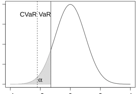
2.1 Graphical representation of VaR and CVaR at confidence levelα . . . 9

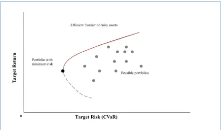
2.2 Efficient frontier of risky assets . . . 10

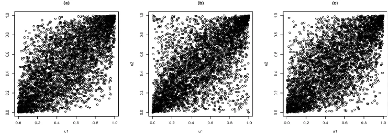
4.1 4000 simulated points from (a) Gaussian copula with ρ = 0.7, (b) t-copula withρ= 0.7,ν=3 and (c) t-copula withρ=0.7,ν=30 respectively. . . 25

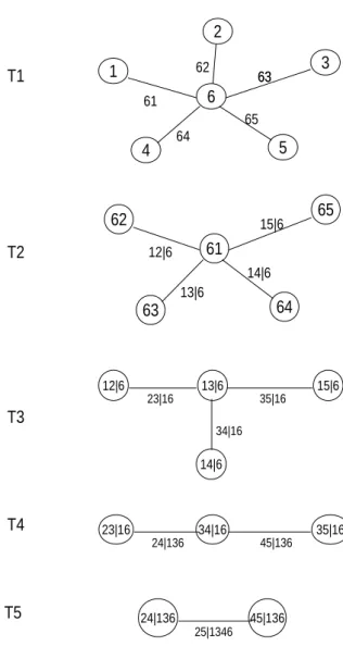
4.2 4000 simulated points from Clayton copula with (a)δ =0.5, (b)δ= 2,(c)δ= 100. 26 4.3 4000 simulated points from Gumbel copula with (a)δ= 1, (b)δ =2,(c)δ =100 28 5.1 A C-vine representation with 6 variables, 5 trees and 15 edges. . . 37

7.1 Optimization with respect to time horizon . . . 48

7.2 Daily log return series of the 6 indices during the period from from 27.03.2005 to 26.03.2008. . . 49

7.3 Normal QQ-plots of the daily log returns of all indices . . . 50

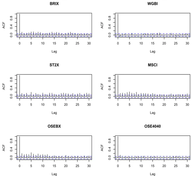
7.4 ACF of the absolute values of the daily log returns of all indices . . . 51

7.5 Selected plots from GARCH(1,1) model fitted for BRIX . . . 55

7.6 Selected plots from GARCH(1,1) model fitted for WGBI . . . 55

7.7 Selected plots from GARCH(1,1) model fitted for ST2X . . . 56

7.8 Selected plots from GARCH(1,1) model fitted for MSCI . . . 56

7.9 Selected plots from GARCH(1,1) model fitted for OSEBX . . . 57

7.10 Selected plots from GARCH(1,1) model fitted for OSE4040 . . . 57

7.11 Canonical vine structure for the sample data for estimation period [200-949] . . 60

7.12 Canonical vine structure for the sample data for estimation period [358-1107] . 61 7.13 Efficient frontier Scenario 1 . . . 63

7.14 Portfolio weights of each assets . . . 64

7.15 Efficient frontier Scenario 2 . . . 65 ix

x LIST OF FIGURES

7.16 The accumulation of wealth if 100 NOK is invested using the asset positions resulted from CVaR optimization Scenario 1, Constant-Mix strategy or Buy-and-Hold strategy. . . 67 7.17 The accumulation of wealth if 100 NOK is invested using the asset positions

resulted from CVaR optimization Scenario 2, Constant-Mix strategy or Buy-and-Hold strategy. . . 68

List of Tables

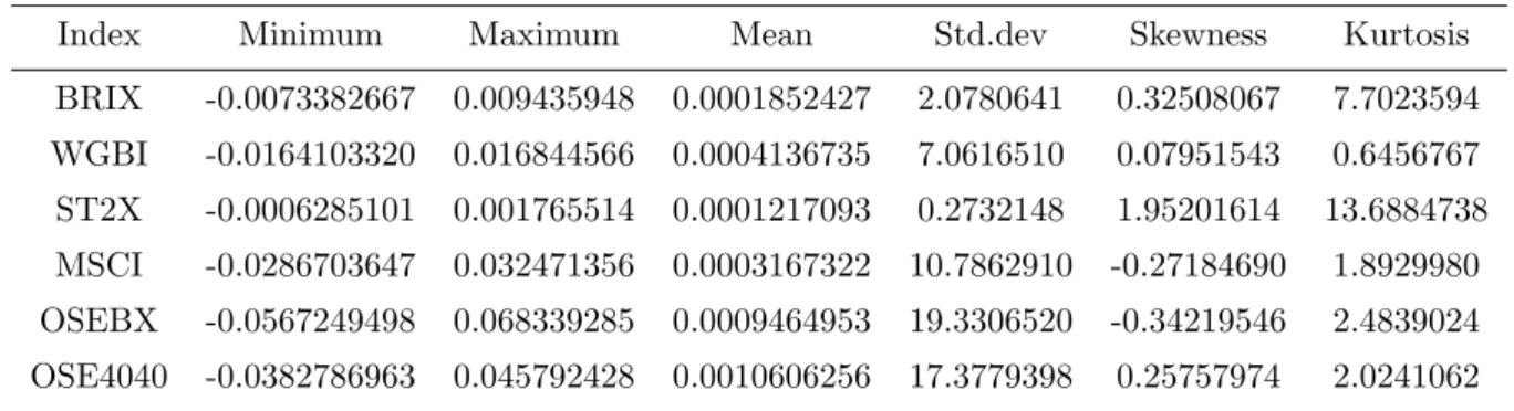
7.1 Preliminary descriptive statistics of the daily log-returns . . . 50 7.2 Estimated parameters for the Norwegian bond index (BRIX) using the GED

as error distribution in the GARCH (1,1) model . . . 52 7.3 Estimated parameters for the World citigroup bond index (WGBI) using the

GED as error distribution in the GARCH (1,1) model . . . 52 7.4 Estimated parameters for the Government Bond Index (ST2X) using the Skew

Student’s t as error distribution in the GARCH (1,1) model.. . . 53 7.5 Estimated parameters for the Morgan Stanley World Index (MSCI) using the

Student’s t as error distribution in the GARCH (1,1) model . . . 53 7.6 Estimated parameters for the Oslo Stock Exchange main index (OSEBX) using

the Student’s t as error distribution in the GARCH (1,1) model . . . 54 7.7 Estimated parameters for the Oslo Stock Excange Real estate index (OSE4040)

using the Student’s t as error distribution in the GARCH (1,1) model . . . 54 7.8 Empirical Kendall’s tau computed pairwise for estimation period [1-750] . . . . 58 7.9 Empirical Kendall’s tau computed pairwise for estimation period [200-949]. . . 58 7.10 Empirical Kendall’s tau computed pairwise for estimation period [358-1107] . . 59 7.11 Sums of the absolute values of empirical Kendall’s taus for selected estimation

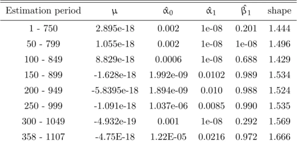
periods. . . 59 7.12 Estimated parameters for PCC C-vine structure for estimation period [200-949] 62 1 Complete list of Portfolio weights for Scenario 1. . . 79 2 Complete list of Portfolio weights for Scenario 2. . . 91

Chapter 1

Introduction

In investment decision making portfolio optimization is an important process of diversification of which proportions of financial instruments held in a portfolio are determined to achieve a maximum expected return contingent on a desired level of risk. The classical approach, known as modern portfolio theory (MPT) started by Markowitz [1952] aim to optimize a portfolio’s expected return with respect to variance as risk measure. This Mean-Variance framework is the foundation for later developments in portfolio optimization. As investors are most concerned about potential losses and its extent, the risk measure of interest is not necessarily the one that regards the overall market price dispersion on average like variance, but rather specifically the negative divergence. Hence alternative risk measures other than variance are introduced and researched subsequently.

Value-at-Risk (VaR) is a very popular risk measure first proposed by Baumol [1963]. It gives an indication of the worst scenario of loss for a given time horizon at a given confidence level. VaR has been widely used as the acceptable risk measure by many financial institutions and regulators, such as the Basel Committee on Banking Supervision. However, as financial return series are often not well presented by a elliptical or normal distribution, VaR is not a coherent risk measure according toArtzner et al.[1999] due to its undesirable mathematical properties such as non-subadditivity and non-convexity. R.McKay and T.E.Keefer[1996] also points out that VaR can be ill-behaved as a function of portfolio posistion as it can display multiple local extrema, creating difficulty for determining the optimal combination of risk factors. Taking such shortcomings into account,Rockafellar and Uryasev [2000] proposed a new approach to portfolio optimization using Conditional Value-at-Risk (CVaR) as the risk measure. CVaR quantifies the mean loss exceeding VaR and is proved to be a coherent risk measure inPflug[2000]. Moreover,Rockafellar and Uryasev[2002] points out that it provides optimization short-cuts when dealing large-scale calculations through linear programming1

1_{Technical background of linear programming is outside the scope of thesis, for details see for exampleKall}

2 CHAPTER 1. INTRODUCTION

techniques, that otherwise could be non-feasible in practice.

This thesis employs the Mean-CVaR methodology introduced by Rockafellar and Urya-sev [2000] to optimize a typical portfolio for a Norwegian life-insurance company. As the topic concerns investment choices and asset allocation we primarily aims at optimizing the portfolio’s expected return by evaluating market risk with CVaR.

As the CVaR optimization procedure uses return scenarios as input, we carry out simu-lations generated from a model fitted to historical data. This requires therefore appropriate modeling of financial return series and their interdependence structure. It is commonly ac-knowledged that return series in financial markets are not independently identically normal distributed but leptokurtotic and subject to volatility clustering. These are important factors to be considered when calculating the risk a portfolio faces. It is a well known phenomenon that volatility varies over time and that it tends to come in clusters; appearing periods of low volatility and periods of high volatility. It is also shown that the volatility of financial time series are autocorrelated; that is, current volatility depends on past volatility. Since the volatility is not directly observable, it is essential to have an adequately good model for estimation and forecast. We will apply the most widely used model, GARCH(1,1) introduced byBollerslev [1986] to model the volatility of univariate return series.

Additionally, in order to accurately estimate the CVaR of the portfolio, we need to ef-fectively capture the dependence structure between the asset returns, especially in the tails where extreme events may occur concurrently. Copulas allow one to model the dependence structure and margins separately, and therefore provide more flexibility. This thesis will use the general theoretical framework of copula and apply the pair-copula construction (PCC) and vine structure introduced by Bedford and Cooke [2002] to model the interdependence between the residuals of the return series.

Since the introduction of CVaR as alternative risk measure, there has been extensive research comparing the CVaR portfolio optimization and Markowitz [1952]’s Mean-Variance approach such asAas and Low[2012] and Deng et al.[2011]’s work. We, on the other hand, investigate the performance of the CVaR optimized portfolio in terms of rebalancing strategy by comparing other asset allocation strategies such as Constant-Mix and Buy-and-Hold.

This thesis is structured as follows. In Chapter 2 we present a summary of the CVaR optimization methodology. Chapter 3 describes the univariate GARCH model in the context of volatility clustering in the financial market. Chapter 4 introduces the general theoreti-cal framework of copulas while Chapter 5 details the pair-copula composition (PCC) and canonical vine structure of a general multivariate distribution and its parameter estimation. In Chapter 6 we outline the portfolio optimization problem by combining the PCC-GARCH and Mayer [2011]

3

model with CVaR optimization, while we carry out the empirical analysis in Chapter 7. Fi-nally, the conclusion and suggestions for future work are presented in Chapter 8.

Chapter 2

Portfolio Optimization

The concepts of modern portfolio theory dates back to Markowitz [1952]’s introduction of risk management through portfolio diversification and selection based upon efficient frontier. The traditional framework of optimization is based on the use of variance as the measure of financial risk. The return of a portfolio is considered as a random variableRand modeled as a weighted sum of asset returnsr1, ...,rn,

R =

n

∑

i=1

wiri,

wherewirepresents the weights of each asset in the portfolio subject to the constraint n

∑

i=1

wi =

1. As the Markowitz framework uses the sample mean and variance as estimates for return and risk, minimizing the variance-covariance of the assets yields a set of feasible portfolios bounded by a curved line called the efficient frontier. The efficient frontier represents the set of optimal portfolios that generate the highest expected return for a given level of risk, or the lowest expected risk for a given return. As a result, one can construct at least one optimal portfolio from the available instruments with the expected return and risk corresponding to the point along the efficient frontier.

However, the Mean-Variance portfolio optimization has several drawbacks as the resulting efficient frontier relies on the sample estimates that are computed under the assumption of multivariate normality. Hence, unless the asset returns are normally distributed, which is highly improbable in practice, it is inappropriate to estimate risk by sample variance as it does not capture fat tails and skewness in the underlying distribution. Moreover, the variance accounts for both downside and upside movements in asset returns equally whilst the intention of risk management is to capture downside risk, that is, the risk of loss.

More recently, other risk measures such as at-Risk (VaR) and conditional Value-at-risk (CVaR) have been used in portfolio optimization. This thesis employs the approach

6 CHAPTER 2. PORTFOLIO OPTIMIZATION

introduced byRockafellar and Uryasev[2000] where the expected portfolio return is optimized by minimizing CVaR. The following sections give an overview of the basic concepts in risk management prior to illustrating the CVaR optimization problem.

The main references in this chapter areMarkowitz[1952],Artzner et al.[1999],Rockafellar and Uryasev[2000], Krokhmal et al. [2002],McNeil et al. [2005],Morgan[1996],W¨urtz et al. [2009],G.Cornuejols and Tutuncu[2006] and Aas and Low[2012].

2.1

Risk Concepts

Morgan [1996] defines risk as the degree of uncertainty of future net returns. In the context of finance and insurance there are three main risk categories to be considered, namely,credit risk;market risk andoperational risk. Credit risk is the risk of loss of financial capital such as loan repayments due to the failure of a borrower to meet contractual obligations, commonly known as thedefault. Credit risk arises from situations where a current debt or investment is expected to receive future cash payments. Consequently, investors or lenders require interest payment to compensate such risk of default of the borrower. The greater the credit risk, the higher the interest rate. Credit risk is therefore closely related to interest rate as a way of evaluating a borrower’s ability to meet scheduled payment obligations. Market risk is the risk of losses in financial positions due to adverse movements in market prices affected by factors such as economic recession, political unrest and events that have substantial impact on the overall performance of the financial markets. This type of risk is omnipresent in various financial sectors and cannot be eliminated, it is however, possible to hedge against market risk by diversification. It is now a common practice to diversify a portfolio across different industries as opposed to financial markets since they have become increasingly correlated as a result of globalization. Operational risk refers to the risk of operational failures due to inadequate internal processes, systems and human errors.

Although insurance companies are certainly exposed to insurance risk that arises from a policyholder’s mortality and morbidity status, the most critical risk associated with asset allocation and portfolio management is market risk. Notably, comprehensive market risk management involves techniques such as stress testing, worst scenario analysis combined with careful use of statistical risk measures. In the context of portfolio optimization, the scope of this thesis covers only the statistical approach to risk measurement.

2.2. RISK MEASURES 7

2.2

Risk Measures

Selection of appropriate risk measures is central to optimization problem. A good risk mea-sure should therefore have a list of desirable properties. This leads to the concept of so-called coherent risk measures presented by Artzner et al. [1999]. Letρ(·) be the risk measure and letR1 and R2 be two random variables representing for example, two assets in a portfolio. A risk measure is coherent if it satisfies the following axioms:

Axiom T - Translation invariance

ρ(R1+l) =ρ(R1)−l (2.1)

Axiom S - Subaddivity

ρ(R1+R2)≤ρ(R1) +ρ(R2) (2.2) Axiom PH - Positive homogeneity

ρ(lR1) =lρ(R1) (2.3)

Axiom M - Monotonicity

ρ(R1)≤ρ(R2),R2≤ R1 (2.4) Axiom T states that adding a quantitylto an asset reduces the risk by the equivalent amount. Axiom S reflects the idea that risk can be reduced by diversification. The total risk faced by a portfolio is less than or equal to the sum of the risks of its individual assets. Axiom PH says that if one increases the amount invested in one asset one increases the risk with the same factor. Axiom M means that if the value ofR1in general is larger than that ofR2, then the risk of R1 is less than or equal to that of R2. Note that Axiom S and Axiom PH together ensures the convexity of a risk measure, which implies that if there exists a local minimum, it is also the global minimum. Convexity and subadditivity are important properties of risk measures used for solving optimization problems. In particular, convex and continuously differentiable functions are easy to minimize numerically as addressed in Rockafellar and Uryasev[2000].

Banking laws and regulations issued by current financial regulators formulate risk measures as percentiles of the loss distribution, such as Value-at-Risk (VaR). Basel II for examples, con-siders Value-at-Risk (VaR) as the preferred risk measure. However, VaR has its shortcomings as it is only a coherent risk measure when the underlying assets follow normal or lognormal distributions. It is otherwise unstable and difficult to handle numerically when dealing with

8 CHAPTER 2. PORTFOLIO OPTIMIZATION

heavy tailed distributions as stressed by Rockafellar and Uryasev [2002]. The following sec-tion introduces the concept ofConditional Value-at-Risk (CVaR) as an alternative statistical measure of market risk.

2.2.1 Conditional Value-at-Risk

Often considered as an upper bound for Value-at-Risk (VaR), CVaR estimates the extent of loss on average given a loss occur. In order to understand the concept of CVaR, we first need to define VaR, a measure of the maximum potential change in portfolio value for a given probability over a fixed time horizon ∆. Generally, CVaR is the weighted average of loss exceeding VaR at some confidence level. In the case of a continuous distribution it is simply the expected loss that exceeds VaR. CVaR is thus also known asexpected shortfall. Consider a portfolio ofn instruments over a time period ∆. Then, the loss function is the negative of the return of the portfolio, where portfolio return is given as the sum of returns on individual instrumentsr scaled by weightsw

fL(w,r) =−(w1r1+· · ·+wnrn) =−wTr (2.5)

We define then the probability of the loss fL(w,r)not exceedingl as

Φ(w,l) =

Z

fL(w,r)≤l

p(r)dr, (2.6)

where p(r)is the joint density function of the random returns and Φ(w,l)is the cumulative distribution loss function associated withwand is continuous and non-decreasing with respect to l.

The idea behind Value-at-Risk (VaR) is to consider the worst case scenario. Investors are interested in odds of large losses. VaR is an estimate of the maximum expected loss at a given confidence level over a fixed time period ∆. For instance, for an investment of 100$ daily, a 95%-VaR of −6% can be interpreted as we are 95% confident that the daily loss will not exceed6$. Formally, VaR with respect to the portfolio weightswfor a given confidence level

α ∈(0, 1)is given by the smallest lsuch that the probability of the loss fL(w,r)exceedingl

is at most 1−α

VaRα(w) =min{l:Φ(r,l)≥α}. (2.7)

Although VaR is widely used for measuring downside risk, it does not account for scenarios exceeding VaR. In other words, VaR does not distinguish the extent of losses beyond the threshold. Furthermore, it does not satisfy all Axioms in (2.1)-(2.4), the criterion for coher-ence. It has undesirable properties such as non-subadditivity and non-convexity which fails to support the idea of diversification. With non-subadditivity we mean that the VaR of a

2.2. RISK MEASURES 9

portfolio is not necessarily bounded above by the sum of the VaR of the the individual assets. In other words, a diversified portfolio could be exposed to more risk and hence higher capital requirement than a less diversified one. Furthermore, the non-convex characteristic of VaR means that a local minimizer of VaR does not necessarily imply a global minimum. Conse-quently, VaR has its limitation as a risk measure for the portfolio optimization problem. An illustration of VaR and CVaR is given in figure 2.1.

−4

−2

0

2

4

0.0

0.1

0.2

0.3

0.4

X

Density

VaR

CVaR

α

Figure 2.1: Graphical representation of VaR and CVaR at confidence levelα

Formally, the CVaR associated with the portfolio weights wfor a given confidence level

α ∈[0, 1] is defined as CVaRα(w) = 1 1−α Z fL(w,r)≥VaRα(w) fL(w,r)p(r)dr (2.8)

Notably, the probability of fL(w,r) exceeding or equal to VaRα(w) accumulates to 1−α.

The definition of CVaR also ensures that VaR≤ CVaR, hence minimizing CVaR of a port-folio naturally implies a low VaR as well. Besides the properties mentioned above, the value

CVaRα(w) also behaves continuously with respect toα ∈ [0, 1]. This is another feature of

CVaR that makes it advantageous to VaR, itsstability in the event of fat-tailed loss distribu-tions. (for detailed proof see Rockafellar and Uryasev [2002]).

10 CHAPTER 2. PORTFOLIO OPTIMIZATION

2.3

Efficient frontier

In the event of portfolio selection, we are faced with all possible combinations of assets in a risk-return space. The efficient frontier, in the shape of hyperbola, highlights a set of optimal portfolios with the greatest expected return given a risk level, or those with lowest risk level for a given expected return. In other words, the efficient frontier pinpoints the intersection between the portfolios with maximum return and those with minimum risk.

Figure 2.2 illustrates an example of the efficient frontier. The region on the right-hand side of the curve shows the set of all attainable portfolio combinations. The black dot is identified as portfolio with minimum risk. For the same level of risk, investors would always prefer the portfolio with higher expected return; given the different expected return investors would also prefer the portfolio with a higher return and a lower level of risk. Therefore, the efficient frontier is represented by the solid red curve starting from the portfolio with minimum risk and along the upward slope.

0

Efficient frontier of risky assets

Target Risk (CVaR)

Ta rg et Re tu rn Feasible portfolios Portfolio with minimum risk

2.4. MEAN-CVAR PORTFOLIO OPTIMIZATION 11

2.4

Mean-CVaR Portfolio Optimization

Rockafellar and Uryasev[2000] introduces their approach to portfolio optimization that com-putes VaR and optimizes CVaR in terms of the following function:

Fα(w,l) =l+ 1 1−α Z fL(w,r)≥l (fL(w,r)−l)p(r)dr. (2.9)

Alternatively, it can also be formulated as following:

Fα(w,l) =l+

1

1−αE{[fL(w,r)−l]

+_{} (2.10)}

where[fL(w,rs)−l]+= max[fL(w,rs)−l, 0]. This function Fα(w,l)oflis a convex function

that has the following crucial properties:

VaRα(w)∈arg min

l Fα(w,l), (2.11)

CVaRα(w) =min

l Fα(w,l). (2.12)

In other words,CVaRα(w)is the minimum value of Fα(w,l)and VaRα(w), belonging to the

non-empty, closed and bounded set of l for which the minimum is attained, is a minimizer of

Fα(w,l).

Note that the joint density p(r)is often not known. Hence historical values of returns or simulated return scenarios r1, ...,rs using the volatility and correlation estimates for the

un-derlying portfolio assets are instead used. Therefore, Rockafellar and Uryasev[2000] approx-imate the integral in equation (2.10) by sampling the probability distribution of r according to density p(r). As a result, the corresponding approximation to Fα(w,l)based on scenarios

s=1, ...,S is then ˜ Fα(w,l) =l+ 1 (1−α)S S

∑

The functionF˜α(w,l)can then be transformed into a linear expression by replacing(fL(w,rs)− l)+ with a dummy variable Zs. We can hence solve the optimization problem by minimizing

the following l + 1 (1−α)S S

∑

subject to the following set of linear constraints:

Zs ≥ fL(w,rs)−l. (2.15)

Zs ≥0, (2.16)

12 CHAPTER 2. PORTFOLIO OPTIMIZATION

wT_{1=1 (2.18)}

w≥0. (2.19)

W¨urtz et al. [2009] stress that constraints (2.15) and (2.16) alone cannot ensure Zs = (fL(w,rs)−l)+. However, it is justified that since the function to be minimized involves

a positive multiplier of Zs, an optimal solution can only be found whenZsis the maximum of fL(w,rs)−l and 0. Constraint (2.17) implies that the expected return on a portfolio should

be bounded below by an arbitrary value R. Constraint (2.18) simply says that the sum of the weights of a portfolio should be 1. Constraint (2.19) ensures that all assets in the portfolio take long position, that is no short-selling. This constraint can modified according to portfolio strategy.

2.5

Compared to Mean-Variance Portfolio Optimization

Rockafellar and Uryasev [2000] has shown that the Mean-Variance (MV) and CVaR ap-proaches to selecting optimal portfolio generates the same efficient frontier in case of a nor-mally distributed loss function. However, differences arise when the underlying loss distribu-tion is characterised by non-normality and asymmetry.

Consider the same portfolio of n instruments, the MV optimization problem aims to minimize the portfolio variance

wTΣˆw (2.20)

subject to the constraints

wTE(r) =R (2.21)

wT1= 1. (2.22)

Here, the vector w denotes portfolio weights of each instrument, matrix Σˆ represents an estimate of the covariance between returns of the instruments, and Ris the target return.

For a given return,Krokhmal et al.[2002] has shown that the CVaR optimal portfolio has a higher standard deviation than that of the efficient MV portfolio. Whilst the MV optimal portfolio has higher CVaR than that of CVaR portfolio. As the confidence level increases the discrepancy between the two approaches also increases.

Chapter 3

GARCH

In finance, volatility is an important concept that measures the movements in market prices. It is therefore an important factor for investors to take into account when calculating the risks they face. It is a well known phenomenon that volatility varies over time, and that it tends cluster in periods of low volatility and periods of high volatility. It is also shown that the volatility of financial time series is autocorrelated, that is, current volatility is dependent on the past.

Since volatility is not directly observable, it is therefore essential to be able to estimate and predict volatility with a good model. Much literature has been written about the model-ing of univariate volatility. This chapter presents thegeneralized autoregressive conditionally heteroscedastic (GARCH) model introduced by Bollerslev [1986] as a practical tool for fore-castingvolatility of a financial time series that varies over time. We concentrate on univariate GARCH models. Multivariate GARCH models are not considered in the context of this thesis as we will use copula instead for modeling time-varying dependencies.

The main references in this chapter areAas and Dimakos[2004],Bollerslev[1986],McNeil et al.[2005],Zivot and Wang[2006],Posedel [2005],Bradley and Taqqu[2003] andFernandez and Steel [1998].

3.1

Volatility

In times of stress market prices tend to fluctuate to a great extent and the magnitude of successive price movements are increasingly correlated over time. Note that when studying the magnitude of consecutive price movements we consider the logarithmic differences of market prices or indices, known as log-returns. The advantage of log-scaling is that compounded log-returns can be conveniently computed by summation. For example, annual log-returns are simply given as the sum of daily log-returns. Formally, a time series of daily log-returns

14 CHAPTER 3. GARCH

{Xt}t∈Z is expressed as

Xt= ln(Pt)−ln(Pt−1) (3.1) where{Pt}t∈Z are observed market prices. Unless otherwise specified, the use of termreturns all refers to log-returns.

For a stochastic process {Xt}t∈Z representing returns from financial market variables, its variance conditioned on the history{Ft−1}t∈Z,1

Var(X_t|F_t−1),

is not constant over time due to the presence of volatility clustering. Formally, volatility is defined as

σ_t= pVar(Xt|Ft−1). (3.2)

Volatility clustering can be detected by computing the autocorrelation function of the absolute and/or squared values of returns defined as follows,

ρ_abs(h) = p Cov(|Xt|,|Xt−h|) Var(|Xt|)Var(|Xt−h|) = γabs(h) γ_abs(0), (3.3) ρ_squared(h) = Cov(X 2 t,Xt2−h) q Var(X_t2)Var(X_t2_−h) = γsquared(h) γ_squared(0). (3.4)

Here, h ≥0 denotes the lag in time and ρ(h) =ρ(−h), which means that autocorrelation is an even function. An autocorrelation function with positive values for a large amount of lags implies volatility clustering.

In general, characteristics of log-returns on indices, interest rates, commodity prices and other financial instruments are characterized by the following so-called stylized facts:

1. Return series are not independently identically distributed.

2. Return series are heavy, fat-tailed and asymmetric, hence, not Gaussian. 3. Absolute or squared values of return series display strong serial correlation. 4. Volatility is time varying and extreme values appear in clusters.

5. Volatility is mean-reverting, that is, in the long run it will settle down to a certain level. The following sections focus on the technique used for modeling financial returns with time-varying volatility: GARCH-models, in particular, the widely used GARCH(1,1) model.

1_{Conditioning overF}

3.2. GARCH PROCESS 15

3.2

GARCH process

The method of modeling time-varying conditional variance (squared volatility) was first intro-duced byEngle[1982] with the ARCH (Autoregressive Conditional Heteroskedastic) process. This model separates unconditional and conditional variance, where the latter is allowed to vary over time as a function of historical errors, also known as residuals. To illustrate, let {Xt}t∈Z be a stochastic process of asset daily returns in terms of sample expected returns and residuals:

Xt =µ+t

(3.5)

An ARCH(p)process is given by

_t=σ_tzt, σ_t2=α₀+ p

∑

where zt is iid W N(0, 1) 2 and α0 > 0,αi ≥ 0,i = 1, ...,p. Given accruals of information

Ft−1,σt is known at time t and this ensures that

E[_t|F_t−1] =E[σtzt|Ft−1] =σtE[zt|Ft−1] =σtE[zt] =0 (3.7)

Var[_t|F_t−1] =E[σ_t2z2_t|Ft−1] =σ_t2E[zt|Ft−1] =σ_t2E[zt] =σt2 (3.8)

A few years later Bollerslev [1986] introduced the GARCH model as an extension to the ARCH process to ”allow for both a longer memory and a more flexible lag structure.” Bollerslev [1986] Consider the same stochastic process {Xt}t∈Z defined in Equation (3.5). A GARCH(p,q)process is formally defined as

_t =σ_tzt, σ_t2 =α₀+ p

∑

∑

where zt is iid W N(0, 1) and α0 > 0,αi ≥ 0,i = 1, ...,p,βj ≥ 0,j= 1, ...,q. For q = 0 the

process reduces to the ARCH(p)process. Note that the ARCH process expresses the condi-tional variance (squared volatility) as a linear function of the pastp-period squared residuals

2_t−i only, whilst the GARCH process allows the conditional varianceσ_t2 to be dependent on the pastq-period conditional variancesσ_t2_−j in addition to the past p-period squared values of residuals.

2_{z

t}is a white noise process if{zt}is a sequence of uncorrelated random variables, each with mean0and

16 CHAPTER 3. GARCH

3.2.1 GARCH(1,1)

In practice, the most commonly used univariate GARCH model is the simplest GARCH(1,1) model given by

_t =σ_tzt,

σ_t2 =α₀+α₁2_t−1+β₁σ_t2₋₁

(3.10)

where zt is iid W N(0, 1) and the three parameters satisfy 0 <α0, 0 ≤α1 ≤ 1, 0 ≤ β1 ≤ 1 andα₁+β₁ ≤ 1. The GARCH(1,1) model provides an adequate fit to financial time series and produces the stylized facts presented in previous section. Notably, the variance process

σ_t2in GARCH(1,1) is(weakly) stationary3 ifα₁+β₁ <1. To forecast future volatility, we are interested in predictingσ_t+h forh≥ 1. Formally, it translates into the following information F_t which isknown at timet:

E[σ_t2₊₁|F_t] =α₀+α₁E[2_t] +β₁E[σ_t2] =α₀+ (α₁+β₁)σ_t2.

3_{A time series{X}

t}t∈Z is weakly stationary if it satisfies the following:

E(X2_t)<∞, E(Xt) =µ,

cov(Xt,Xt+h) =γx(h),∀t

3.3. NON-GAUSSIAN ERROR DISTRIBUTIONS 17

When looking h > 1 steps forward, we proceed to follow a recursive scheme step-wise and this yields a general formula as follows:

E[σ_t2₊₂|F_t] =α₀+α₁E[2_t+1] +β₁E[σ_t2₊₁] =α₀+ (α₁+β₁)E[σ_t2₊₁] =α₀+ (α₁+β₁)[α₀+ (α₁+β₁)σ_t2] =α₀[1+ (α₁+β₁)] + (α₁+β₁)2σ_t2 E[σ_t2₊₃|Ft] =α0+α1E[2t+2] +β1E[σt2+2] =α₀+ (α₁+β₁)E[σ_t2₊₂] =α₀+ (α₁+β₁)hα₀[1+ (α₁+β₁)] + (α₁+β₁)2σ_t2 i =α₀[1+ (α₁+β₁) + (α₁+β₁)2] + (α₁+β₁)3σ_t2 · · · E[σ_t2_+h|Ft] =α0[1+ (α1+β1) + (α1+β1)2+· · ·+(α1+β1)h−1] + (α1+β1)hσt2 =α₀ h−1

∑

As h−→∞, we obtain the stationary variance E[σ_t2_+h|Ft]−→

α₀

1−α₁−β₁. In other words,

this is the long-run level where volatility will mean-revert to for a stationary GARCH(1,1) model. Furthermore, the sum of parametersα₁ and β₁ are often known as persistence that describes how quickly volatilities decay after a shock in financial markets. Sinceα₁+β₁ <1, forh steps ahead in time, we have(α₁+β₁)h −→0 ash−→∞. The pace of convergence is therefore dependent ofα₁+β₁, the closer the size of persistence to 1, the longer it takes for a shock to be forgotten in the market.

3.3

Non-Gaussian Error Distributions

When modeling the volatility of return series with GARCH models one needs to consider both the marginal distribution which is the distribution of errors_tand the conditional distribution which is the distribution of_t/σ_t. Financial time series such as daily log-returns are known for displaying fat and heavy-tailed characteristics that are non-Gaussian. GARCH models with conditionally normally distributed errors are therefore sometimes unable to provide a good

18 CHAPTER 3. GARCH

fit accounting for asymmetry and leptokurtic shape of marginal distribution. Consequently, alternative error distributions are considered depending on the class of asset returns. The following section give an overview of three alternative conditional distributions in univariate case: Generalized Error Distribution, standard Student’s t-distribution and skew Student’s t-distribution.

3.3.1 Generalized Error Distribution

Thegeneralized error distribution (GED) first introduced by Nelson (1991) is an example of distribution to capture fat tails. Formally, the density of a GED variable with mean zero and variance one is given by

fν(z) = νexp[−(1/2)|z/λ|ν_] λ2ν+1ν Γ(1/ν) , (3.11) where λ= " 2−2/νΓ(1/ν) Γ(3/ν) #1₂ (3.12)

and ν > 0 is the shape parameter that controls the thickness of the tail. When ν = 2, the GED density function becomes the standard normal; when ν > 2, the distribution of x has thinner tails than that of normal distribution; and whenν < 2, x has thicker tails than the normal. When ν−→∞ the GED density function approaches to the uniform distribution.

3.3.2 Student’s t-distribution

The Student’s t distribution is a another commonly used fat-tailed distribution for modelling asset returns. The classical Student’s t density is symmetric and have a single peak like the normal distribution. Formally, the density function of the standard student’s t-distribution is given by fν(z) = Γ(ν+₂1) Γ(ν₂)√πsν 1+ z 2 sν −ν+1₂ , (3.13)

where ν is the degrees of freedom that controls the thickness of the tails and s the scale parameter. As the number of degrees of freedom increases, the t-distribution approaches the standard normal distribution. The mean and variance of the Student’s t distribution are

E(Z)=0,ν>0

Var(Z) = sν

ν−2,ν>2

Since the error termzt in a GARCH model following Student’s t-distribution has variance 1

conditional on past events, the scale parameters under the standard t-distribution must then be (ν−2_ν ).

3.4. PARAMETER ESTIMATION 19

Note that although both Generalized Error Distribution GED and standard Student’s t-distribution account for fatter tails than that of the normal distribution, they are still symmetric. To account for any skewness and asymmetry, suitable alternative would be for example, the skew Student’s t-distribution.

3.3.3 Skew Student’s t-distribution

There are several differentskew Student’s t-distributions. We will use theFernandez and Steel [1998] version in the context of this thesis. The probability density function is given by

f(z) = 2 γ+_γ1 fν( z γ)I[0,∞)(z) + fν(γz)I(−∞,0)(z) . (3.14)

Here I(·)is the indicator function and fν(·)is the PDF of standard Student’s t-distribution.

γ > 0 is the skewness parameter and when γ = 1, the skewness is 0 and f becomes the standard Student’s t distribution withν degrees of freedom.

3.4

Parameter Estimation

In practice, parameter estimation of GARCH models is performed on the basis of historical data. The most commonly used approach is maximum likelihood. We are interested in finding estimates that maximize the probability of which generates the set of known data. The likelihood is constructed and computed conditional on accruals of past information and volatilityσ_t defined recursively in terms ofσ_t−1.

As the parameter estimates are dependent of the historic data used for fitting GARCH models, the behaviour of estimates needs to be distinguished with respect to the underlying distribution. Consequently, this leads to the following two methods of GARCH model es-timation: maximum likelihood estimation (MLE) and quasi-maximum likelihood estimation (QMLE). In MLE, the likelihood function uses the true distribution of data. This method generates estimates that contain more information. The challenge is, however, that it requires the distribution of the data set to be known, which in practice is difficult to obtain. In QMLE, on the other hand, we do not know the true distribution of the data set, but assume the error term is asymptotically i.i.d Gaussian distributed given all past information. This method is adequate to obtain good parameter estimates and is more practical and easier to implement. To illustrate MLE, consider the GARCH(1,1) model specified in Equation(3.8). We assume nowztis i.i.d standard normal, hencetconditional on past information will follow a Gaussian

distribution with mean 0and varianceσ_t2. The conditional density function is then given by

f(_t|F_t−1) = √ 1 2πσ_te

−2t

20 CHAPTER 3. GARCH

Let Θ = (α₀,α₁,β₁) be the parameter vector. Then, the log-likelihood function of the GARCH(1,1) model conditional on historic values is

l(Θ) = n

∑

∑

whereσ_t = qα₀+α_1t2₋₁+β₁σ_t2₋₁. Note that both methods require a starting value forσ₀

in order to carry the numerical maximazition of log-likelihood. The value can often be chosen as the sample variance.

3.5

Simulation

A GARCH(1,1) process with estimated parametersα₀,α₁,β₁ can be generated with the fol-lowing simulation algorithm:

•Simulate z with respect to appropriate conditional distributions:

z∼ gedν(0, 1),or

z∼ tν(0, 1),or

z∼ stν,γ(0, 1).

•Generate sample of T observations using dynamics

σ_t2 =α₀+α₁2_t−1+β₁σ_t2₋₁,

_t =σ_tzt

Note that the algorithm requires an initial value forσ₀ and ₀. They can for example, be chosen as the last estimated value of the GARCH(1,1) process.

Chapter 4

Copulas

While the GARCH model allows us to predict and analyze the volatility of financial time series when it varies over time, we need, in addition, a tool to model the dependence structure between the asset returns.

When studying dependence among random variables, linear correlation is by far the most commonly used measure. However, as it is a measure oflinear dependence, linear correlation is limited to those of multivariate normal and elliptical distributions. Returns from financial markets such as bond indices, exchange rates and equity prices are known for non-normal behavior. Distribution of such returns are often skewed with heavier left tails than under normality, implying greater likelihood of large losses than gains. Hence, measures based on multivariate normal assumption cannot fully account for the dependence structure of financial assets. Alternatively, appropriate modeling of time-varying dependence between assets across financial markets can be performed by the use of acopula.

Copula is Latin for “a link, tie, bond ” (Cassell’s Latin Dictionary) and was first em-ployed in a statistical sense by Abe Sklar (1959). He described copulas as “functions that join or ‘couple´ multivariate distribution functions to their one-dimensional marginal distribution functions”Nelsen [2006]. The advantage of copula-based approach is it provides a way of modeling dependence structure between random variables independently of their margins. That is, a multivariate distribution can be decomposed into marginal distributions that are selected freely and then linked through suitable copulas. Therefore, it provides the opportu-nity to study the marginal distribution functions and the copula separately. Consequently, a given copula can result in various multivariate distributions by selecting different marginal distribution functions.

The following sections give the definition of a copula, examples of different copula fam-ilies and dependence measures derived from copulas. Estimation of copula parameters and simulation from copulas will be presented in the next chapter as the approaches are different

22 CHAPTER 4. COPULAS

in the context ofpair-copula construction.

Main references in this chapter areNelsen[2006],Embrechts et al.[1986],Embrechts et al. [1999],Aas et al.[2007],Aas [2004]McNeil et al.[2005] and Brechmann[2010].

4.1

Definition

A copula can be understood as a function that links univariate marginal distributions to form multivariate distribution functions. A d-dimensional copula is a distribution function on

[0, 1]d with uniformly distributed margins on[0, 1]. Its role for describing dependence among random variables was first introduced in Sklar’s theorem (1959) which states the following: Theorem 4.1. Sklar’s theorem

Let F be a d-dimensional distribution function with margins F1, ...,Fn. Then there exists an

unique copula C such that for all x= (x1, ...,xd)‘∈ Rd,

F(x₁, ...,xd) =C(F1(x1), ...,Fd(xd)). (4.1)

If F1, ...,Fd are continuous, then C is unique; otherwise, C is uniquely determined on RanF1×...Fd. Conversely, if C is a copula and F1,Fd are distribution functions, then the

function F is a joint distribution function with margins F1, ...,Fd.

Now denotexi =F_i−1(ui),i=1, ...,dwhereF_i−1(ui)0sare the inverse marginal distribution

functions. It follows directly that u_i = F_i(x_i). Inserting into (4.1) will give us the following corollary from Sklar’s theorem:

F(F₁−1(u1), ...,F_d−1(ud)) =C(F1(F₁−1(u1), ...,Fd(Fd−1(ud)) =C(u1, ...,ud).

(4.2)

Equations (4.1) and (4.2) show how the copula link marginal distribution functions to form the multivariate distribution and how the copula can be extracted from multivariate distribu-tion funcdistribu-tions, respectively. Note that F_i−1(ui)0s, the inverse marginal distribution functions

are also known as the quantile functions of the marginals. Hence, Equation (4.2) displays

C(u1, ...,ud) as the joint probability of which x1, ...,xd are below their respective u1, ...,ud

-quantiles. The density function f follows also directly by differentiating (2.1) using chain rule

f(x1, ...,xd) =c(F1(x1), ...,Fd(xd))f1(x1)×...× fd(xd) (4.3)

The next section presents examples of copulas from two main categories: elliptical copulas that do not possess a closed form and are implied by well-known multivariate distribution functions; archimedean copulas that have simple, closed, explicit forms and are not derived from well-known multivariate distributions.

4.2. ELLIPTICAL COPULAS 23

4.2

Elliptical copulas

An elliptical distribution has the following density function:

f(x) =cd|Σ|− 1

2g(x−µ)_Σ−1(x−µ), (4.4)

with constant cd , mean vectorµ and covariance matrixΣ.

Elliptical copulas with an absolutely continuous joint distribution function F with con-tinuous, strictly increasing marginals F1, ...,Fd can be constructed as follows. The copula

density cis given by the density of corresponding multivariate distribution function divided by the product of its marginal densities. Formally, it can be expressed by rewriting (2.3) with

xi = F_i−1 fori=1, ...,d defined in (2.2): c(u) = f(F −1 1 (u1), ...,F −1 d (ud)) f1(F1−1(u1))...fd(F_d−1(ud)) . (4.5)

Since elliptical copulas are derived from known distributions, they are therefore also called implicit copulas. The following sections present the two most well-known examples of implicit copulas constructed using the method as shown above.

4.2.1 Gaussian copula

A d-dimensional multivariate Gaussian distributed random vectorX has the representation:

f(x) = 1 (2π)d2|Σ|12

e−12(x−µ)TΣ−1(x−µ)_{, (4.6)}

with mean vector µ and covariance matrixΣ.

The Gaussian copula is constructed from the multivariate standard normal distribution. Hence the mean vectorµbecomes the null-vector and the covariance matrixΣthe symmetric positive definite correlation matrixR∈[−1, 1]d. This yields the multivariate Gaussian copula density according to (2.5) as c(u) = 1 (2π)d2|R|12 e−1/2xTR−1x d ∏ j=1 1 (2π)1/2_e−1/2x2j = e −1 2xTR −1_x |R|1/2_e− 1 2 d ∑ j=1 x2 j , _(4.7) wherex= (Φ−1(u1), ...,Φ−1(ud)).

For simplicity we now consider the bivariate case. The copula density and its correspond-ing distribution function are given as

cρ(u1,u2) = 1 (1−ρ2₎12 exp −ρ 2_(x2 1+x22)−2ρx1x2 2(1−ρ2₎ (4.8)

24 CHAPTER 4. COPULAS Cρ(u1,u2) = Φ−1(u1) Z −∞ Φ−1(u2) Z −∞ 1 2π(1−ρ2₎12 exp −x 2 1−2ρx1x2+x22 2(1−ρ2₎ dx1dx2 (4.9)

whereρ is the parameter of the Gaussian copula.

4.2.2 Student’s t-copula

A d-dimensional multivariate Student t distributed random vector Xhas the representation:

f(x) = Γ[(ν+d)/2] (πν)d/2_Γ(ν/2)|S|1/2 " 1+(x−µ) T_S−1₍ x−µ) ν #−ν+₂d , (4.10)

with mean vector µ,ν>0 degrees of freedom and scale matrix S.

Similar to the Gaussian copula, the t-copula is also based on standard t distribution, hence the mean vector µ becomes the null-vector and the scale matrix S the correlation matrix R∈[−1, 1]d. This yields the t-copula density according to (4.5) as following

c(u) = Γν+d 2 (πν)d/2_Γ(ν 2)|R|1/2 1+ x‘R −1_x ν !−ν+₂d d

∏

∏

wherex = (t_ν−1(u1), ...,tν−1(ud)). t−1ν is the inverse standard univariate student’s t-distribution

with expectation 0, variance _ν−2ν andν degrees of freedom.

Now consider the bivariate case again. The Student’s t-copula density function is given by: cρ,ν(u1,u2) = Γ(ν+2 2 )/Γ(ν2) νπdtν(x1)dtν(x2) p 1−ρ2 1+ x 2 1−2ρx1x2+x22 2(1−ρ2₎ − (ν+2) 2 , (4.12)

wheredt(·)andt−1_ν (·)are the probability density and the quantile function of the univariate standard t distribution with linear correlation coefficient ρ and ν > 0 degrees of freedom. The corresponding distribution function for bivariate t copula is

Cρ,ν(u1,u2) = t−1 ν (u1) Z −∞ t−1 ν (u2) Z −∞ 1 2π(1−ρ2₎12 1+ x 2 1−2ρx1x2+x22 2(1−ρ2₎ − (ν+2) 2 dx1dx2. (4.13)

4.3. ARCHIMEDEAN COPULAS 25

The Student’s t-copula has degrees of freedom ν in addition to ρ as parameters compared to the Gaussian copula that only has one parameter, ρ. The degrees of freedom ν has significant contribution to describing extreme co-movements among financial risk factors. The tendency to exhibit joint extreme movements decreases as the degrees of freedom ν

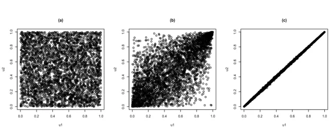
increases. Consequently, one can study the dependence structure among assets regardless of their marginal behaviour. Notably, as the Student’s t distribution approaches normality with increasing degrees of freedom; the Student’s t copula also approaches the Gaussian copula as the degrees of freedom increase. Examples of simulations from the Gaussian and Student’s t-copulas are shown in Figure 4.1. Note the similarity between the Gaussian copula in (a) and the t-copula in (c).

0.0 0.2 0.4 0.6 0.8 1.0 0.0 0.2 0.4 0.6 0.8 1.0 (a) u1 u2 0.0 0.2 0.4 0.6 0.8 1.0 0.0 0.2 0.4 0.6 0.8 1.0 (b) u1 u2 0.0 0.2 0.4 0.6 0.8 1.0 0.0 0.2 0.4 0.6 0.8 1.0 (c) u1 u2

Figure 4.1: 4000 simulated points from (a) Gaussian copula withρ= 0.7, (b) t-copula with

ρ=0.7,ν =3 and (c) t-copula withρ=0.7,ν=30respectively.

4.3

Archimedean copulas

Archimedean copulas are another important class of copulas that are easily constructed with explicit forms. They are therefore also calledexplicitcopulas. This family of copulas are espe-cially useful for modeling the credit risk of a portfolio. Formally, ad-dimensional Archimedean copula is defined as follows.

Theorem 4.2. Let ϕ be a continuous, strictly decreasing function from [0, 1] to [0,∞] such that ϕ(0) = ∞ and ϕ(1) = 0. ϕ−1 denote the inverse of ϕ such that it is completely monotonic. Then

C(u)=ϕ−1(ϕ(u1) +...+ϕ(ud)) (4.14)

26 CHAPTER 4. COPULAS

ϕ is called the generator of a copula. We now present two of the most commonly used Archimedean copula families in bivariate case for the simplicity of expression.

4.3.1 Clayton copula

The Clayton copula is an asymmetric copula with larger dependence in the negative tail than in the positive. It has a generator ϕ(t) = 1

δ(t

−δ_{−1) that gives ϕ}−1_{(t) = (δϕ(t) +1)}−1

δ.

The density for bivariate Clayton copula can be expressed as

C(u1,u2) = (u₁−δ+u−₂δ−1)

1

δ_, (4.15)

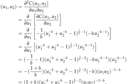
where 0<δ<∞. The copula density can be obtained by differentiating (2.14) with respect to u1 and u2: c(u1,u2) = ∂2C(u1,u2) ∂u₁∂u₂ = ∂ ∂u1 ∂C(u1,u2) ∂u2 = ∂ ∂u₁ −1 δ(u −δ 1 +u −δ 2 −1) 1 δ−1(−δu−δ−1 2 ) = ∂ ∂u1 h (u−₁δ+u−₂δ−1)1δ−1(u−δ−1 2 ) i = (−1 δ −1)(u −δ 1 +u −δ 2 −1) 1 δ−2(−δu−δ−1 1 )(u −δ−1 2 ) =−(1+δ δ )(u −δ 1 +u −δ 2 −1) 1 δ−2(−_δ)(u 1u2)−1−δ = (1+δ)(u−₁δ+u₂−δ−1)δ1−2(u 1u2)−1−δ. (4.16)

δ is the parameter that contains information about dependence structure. Independence is implied by δ −→ 0 whilst perfect dependence is obtained when δ −→_∞. Figure 4.2 shows simulated examples of such limiting cases.

0.0 0.2 0.4 0.6 0.8 1.0 0.0 0.2 0.4 0.6 0.8 1.0 (a) u1 u2 0.0 0.2 0.4 0.6 0.8 1.0 0.0 0.2 0.4 0.6 0.8 1.0 (b) u1 u2 0.0 0.2 0.4 0.6 0.8 1.0 0.0 0.2 0.4 0.6 0.8 1.0 (c) u1 u2

4.3. ARCHIMEDEAN COPULAS 27

4.3.2 Gumbel copula

The Gumbel copula is also an asymmetric copula. However as opposed to the Clayton copula it displays greater dependence in the positive tail than in the negative. Its generator is

ϕ(t) = (−logt)δ _{which yields ϕ}−1_{(t) = e}−(ϕ(t))1δ

. Using the same method, the Gumbel copula distribution function is given by

C(u1,u2) =exp[−((−logu1)δ+ (−logu2)δ)

1

δ]_, (4.17)

where0<δ≤ 1is the parameter for dependence measure. Independence is implied byδ= 1 whilst perfect dependence is suggested when δ −→ 0. Figure 4.3 shows simulations from a Gumbel copula with different values of δ. Similarly, the corresponding copula density can be obtained by differentiating (2.17) with respect to u1 and u2 and is given by

c(u1,u2) = ∂2C(u1,u2) ∂u1∂u2 = ∂ ∂u1 ∂C(u₁,u₂) ∂u2 = ∂ ∂u₁ C(u1,u2)(−1 δ) h (−logu1)δ+ (−logu2)δ i_δ1−1 δ(−logu2)δ−1(− 1 u2 ) = 1 u2 (−logu2)δ−1 ∂ ∂u1 C(u1,u2) h (−logu1)δ+ (−logu2)δ i1_δ−1 = 1 u2 (−logu2)δ−1 C(u1,u2) 1 u1 (−logu1)δ−1 h (−logu1)δ+ (−logu2)δ i(_δ1−1)2 +C(u1,u2)( 1 δ −1) h (−logu1)δ+ (−logu2)δ i1_δ−2 δ(−logu1)δ−1(− 1 u1 ) = 1 u2 (−logu2)δ−1C(u1,u2) 1 u1 (−logu1) δ₋₁h (−logu1)δ+ (−logu2)δ i(1_δ−1)2 +h(−logu1)δ+ (−logu2)δ i1_δ−2 (δ−1) = C(u1,u2) u1u2 (logu1logu2)δ−1 ((−logu1)δ+ (−logu2)δ)2− 1 δ ×h((−logu1)δ+ (−logu2)δ) 1 δ +δ−1 i . (4.18)

28 CHAPTER 4. COPULAS 0.0 0.2 0.4 0.6 0.8 1.0 0.0 0.2 0.4 0.6 0.8 1.0 (a) u1 u2 0.0 0.2 0.4 0.6 0.8 1.0 0.0 0.2 0.4 0.6 0.8 1.0 (b) u1 u2 0.0 0.2 0.4 0.6 0.8 1.0 0.0 0.2 0.4 0.6 0.8 1.0 (c) u1 u2

Figure 4.3: 4000 simulated points from Gumbel copula with (a)δ=1, (b)δ =2,(c)δ =100

4.4

Dependence measures

As addressed inEmbrechts et al.[1999], unless financial returns are presented by multivariate normality or ellipticality the use of linear correlation as dependency measure becomes prob-lematic. Following are some of the limitations of the usual Pearson linear correlation that ought to be repeated and amplified:

1. Correlation is only invariant under strictly increasinglinear transformations, that is,X

and Y do not yield the same correlation aslog(X)and log(Y).

2. Not all values between1 and −1 are necessarily attainable as correlation is dependent on the marginal distribution.

3. A correlation of1 does not necessarily imply perfect positive dependence and a corre-lation of −1 does not necessarily imply perfect negative dependence.

4. Correlation is not defined for random variable with non-finite variances.

This means the use of the linear correlation coefficient as a dependence measure can be misleading when dealing with financial risk factors that are heavy-tailed distributed with non-finite second moments. On the contrary, copulas are invariant under nonlinear continuous and increasing transformation of the margins. This proves to be immensely useful for analysis of financial risk factors as it is common practice to use logarithmic returns on the indices and commodity prices.

This section focuses on two kinds of copula-based dependence measures as alternatives to linear correlation coefficient: concordance andcoefficients of tail dependence.

4.4. DEPENDENCE MEASURES 29

4.4.1 Concordance

As opposed to correlation, concordance does not have the limitations of linear correlation mentioned previously and can be understood as a measure of ”association” that refers to any types of dependence structure between two random variables. According toNelsen[2006] two pairs of random vectors(X1,X2)and(X˜1, ˜X2)are called concordant if(X1−X˜1)(X2−X˜2)> 0, that is X1 < X˜1 and X2 > X˜2. The pairs are discordant if (X1−X˜1)(X2−X˜2) < 0. The following section presents two important measures of concordance: Kendall’s tau and Spearman’s rho.

Kendall’s tau

Kendall’sτfor the random vector(X1,X2)Tis defined as the probability of concordance minus the probability of discordance. Formally, it is defined as

ρτ(X1,X2) =P((X1−X˜1)(X2−X˜2)> 0)−P((X1−X˜1)(X2−X˜2)<0) (4.19) where(X˜1, ˜X2)is independent copy of(X1,X2). IfX1andX2are continuous random variables with a unique copula C, Kendall’s tau can be written as

ρτ(X1,X2) =4

Z Z

[0,1]2C(u1,u2)dC(u1,u2)−1. (4.20)

Notably, for elliptical such as Gaussian and Student’s t-copula Kendall’s tau can be expressed in terms of the linear correlation coefficient ρ as follows:

ρτ(X1,X2) = 2

πarcsinρ (4.21)

For Archimedean copulas on the other hand, Kendall’s tau can be expressed in terms of dependence parameter. For Clayton copula, it is

ρ_τ(X1,X2) =

δ

δ+2 (4.22)

and for Gumbel copula it is

ρτ(X1,X2) =1− 1

δ (4.23)

Spearman’s rho

Spearman’s rho can also be expressed in terms of concordance and discordance. It is formally defined as

30 CHAPTER 4. COPULAS

where X˜1 and Xˇ2 are independent. However, it can be more intuitively understood as the linear correlation between probability-transformed random variables:

ρ_s(X1,X2) =ρ(F(X1),F(X2)). (4.25) IfX1 and X2 are continuous random variables with a unique copula C, Spearman’s rho is given by ρ_s(X1,X2) =12 Z 1 0 Z 1 0 C (u1,u2)dC(u1,u2)−3. (4.26) For elliptical copulas such as the Gaussian and Student’s t-copula, Spearman’s rho is given in terms of the linear correlation coefficient as follows:

ρ_s(X1,X2) = 6

πarcsin

1

2ρ. (4.27)

Unlike the linear correlation coefficient, Kendall’s tau and Spearman’s rho are invariant un-der strictly increasing transformations. Although this is an indication that they are better alternatives as dependence measures, concordance also has its limitations as a dependence measure. For example, different copulas may have the same concordance. Hence, Embrechts et al. [1999] stresses that simple scalar measurement of dependence, both linear correlation and concordance ought to be used with caution. One should instead choose a model for the dependence structure that reflects more detailed knowledge of the risk management in hand. One such alternative is to examine the tail dependence, presented in the following section.

4.4.2 Tail dependence

Kendall’s τ and Spearman’s ρ discussed in previous section measures the amount of overall dependence over the whole unit space [0, 1]2. In risk management, one is also interested in capturing the ”association” between one large value of variable X1 and one large value of another variable X2. This leads to the concept of tail dependence. It refers to the degree of dependence in the corner of the lower-left quadrant or upper-right quadrant of a bivariate distribution. Tail dependence is therefore a measure of dependence between extreme events and proved to be useful for preventing concurrent large losses.

For two continuous random variablesX1 and X2 with marginal distribution functions FX1 and FX2, the coefficient of upper tail dependence is

λ_u(X1,X2) =limα→1P(X2 > FX−12 (α)|X1 >FX−11 (α)). (4.28) Provided that the limit λ_u ∈ [0, 1] exists, the upper tail dependence coefficient describes the probability of large value of X2 given large value of X1. If λu = 0, it implies

4.4. DEPENDENCE MEASURES 31

Analogously, the coefficient of lower tail dependence is

λ_l(X1,X2) =limα→0P(X2 ≤FX−1₂ (α)|X1≤ FX−1₁ (α)). (4.29)

Rewriting the conditional probability in Equation (4.28) the coefficient of lower tail depen-dence can be expressed in terms of a unique bivariate copula C:

λ_l(X1,X2) =lim α→0 P(X2 ≤ FX−1₂ (α),X1 ≤FX−1₁ (α)) X1 ≤FX−1₁ (α)) = C(α,α) α , (4.30)

and the upper tail dependence coefficient can be expressed in terms of a joint survival func-tion1 λ_u(X1,X2) = lim α→1 P(X2 >FX−12 (α),X1> FX−11 (α)) X1 ≤ FX−1₁ (α)) = C¯(α,α) 1−α . (4.31)

Both coefficients have hence the invariance property and are independent of the asset returns margins.

In the case of elliptical distributions, the upper tail dependence coefficient is equal to the lower tail dependence coefficient. The Gaussian copula has probability 0 for joint extreme events regardless of the correlation coefficientρ:

λ_u(X1,X2) =λl(X1,X2) =2 limx→−∞Φ x √ 1−ρ √ 1+ρ =0. (4.32)

The Student’s t-copula is asymptotically dependent in the tails regardless of the value of the linear correlationρ. The tail dependence coefficients are given by:

λ_u(X1,X2) =λl(X1,X2) =2tν+1 −√ν+1 r 1−ρ 1+ρ . (4.33)

Note that stronger tail dependence is implied by lower degrees of freedomνand greater linear correlationρ.

The tail dependence coefficients for Archimedean copulas have simple closed form. The upper tail coefficient for the Clayton copula is zero, λ_u(X1,X2) =0 meaning that it is lower tail dependent. The lower tail dependence coefficient is

λ_l(X1,X2) =2

1

δ. (4.34)

For the Gumbel copula, its lower tail dependence coefficient is zero whilst the upper coefficient is

λ_u(X1,X2) =2−2

1

δ. (4.35)

1_{a joint survival copula is defined asC¯(u}

Chapter 5

Vine-Copula

In theory, construction of higher-dimensional copulas with more than two variables is fully feasible. In practice, however, when dealing with large financial data sets of which not all pairs of risk factors have the same dependence structure, and therefore inequivalent tail dependence; building higher-dimensional copulas is difficult and inflexible. This is due to the limited number of parameters of which most copulas contain, often only one. Consequently, the number of suitable and available parametric higher-dimensional copulas is rather scarce.

This chapter presents the method for modeling the dependence structure for multivari-ate data based on the pair-copula construction (PCC). A pair-wise approach is used since building higher dimensional copulas can be challenging and increasingly difficult with higher dimensions as aforementioned. Since there is a large number of bivariate copulas, the idea is to decompose a multivariate distribution into bivariate copulas as simple building blocks. The structure of thepair-copula decomposition is then illustrated byvines, a graphical model of storing the construction steps and dependence structure presented byBedford and Cooke [2002]. This method of decomposing a multivariate distribution allows us to customize differ-ent pairs of risk factors with various bivariate copulas, while modeling the marginal distribu-tions independent of the dependence structure.

The main references of this chapters areAas et al.[2007],Brechmann[2010],Bedford and Cooke[2002], J.Dißmann et al.[2013] and Schirmacher and Schirmacher[2008].

34 CHAPTER 5. VINE-COPULA

5.1

Pair-Copula Constructions

The concept of pair-copula constructions is based on decomposing an-dimensional joint den-sity functionf as

f(x1, ...,xn) = f(x1)f(x2|x1)f(x3|x2,x1)...f(xn|xn−1, ...,x2,x1). (5.1) Recall Equation (2.3) derived from Sklar’s Theorem stating that the joint density function f can be expressed as a product of the marginal density functions and their corresponding copula densities.

f(x1, ...,xd) =c(F1(x1), ...,Fd(xd))f1(x1)×...× fd(xd).

In the bivariate case, the conditional density function for variable x1 conditioned on variable

x2 can be expressed in terms of pair-copula density and a marginal density

f(x1|x2) =

f(x1,x2)

f(x1)

=c12(F1(x1),F2(x2))f2(x2).

(5.2)

Similarly for the third factor in equation (5.1) we can decompose the three-variable conditional density function as f(x3|x2,x1) =c32|1(F(x3|x1),F(x2|x1))f(x3|x1) =c32|1(F(x3|x1),F(x2|x1))c31(F3(x3),F1(x1))f3(x3), (5.3) or f(x3|x2,x1) =c31|2(F(x3|x2),F(x1|x2))f(x3|x2) =c_31|2(F(x3|x2),F(x1|x2))c32(F3(x3),F2(x2))f3(x3), (5.4)

where c32|1 and c31|2 are two different pair-copula densities. As shown above there are many possible decompositions of the same conditional density function. The number of decompo-sitions increases as the dimension of random variables increases. Following the arguments above, the conditioned density of a variable x conditioned on a vector of variablesv is given by

f(x|v) =c_xvj|v−j F(x|v−j),F(vj|v−j)

f(x|v−j), (5.5)

wherevis ad-dimensional vector of variables . vj denotes a randomly chosen component ofv

and v−j is hence the (d−1)-dimensional vector without the jth componentvj. By iteration,

the construction is straight forward. Moreover, when decomposing a joint density function into marginal densities and pair-copulas there exists numerous choices of conditional densities. As a result, we can have many different re-parametrisations given a unique factorisation which leads to a large number of possible pair-copula constructions.

5.2. REGULAR VINES 35

In order to comput