Similarity measures over refinement graphs

(will be inserted by the editor)

Similarity Measures over Refinement Graphs

Received: date / Accepted: date

Abstract Similarity assessment plays a key role in lazy learning methods such as k-nearest neighbor or case-based reasoning. In this paper we will show how refinement graphs, that were originally introduced for inductive learning, can be employed to as-sess and reason about similarity. We will define and analyze two similarity measures, Sλ andSπ, based on refinement graphs. Theanti-unification-based similarity,Sλ, as-sesses similarity by finding the anti-unification of two instances, which is a description capturing all the information common to these two instances. Theproperty-based

sim-ilarity,Sπ, is based on a process of disintegrating the instances into a set ofproperties,

and then analyzing these property sets. Moreover these similarity measures are appli-cable to any representation language for which a refinement graph that satisfies the requirements we identify can be defined. Specifically, we present a refinement graph for feature terms, in which several languages of increasing expressiveness can be defined. The similarity measures are empirically evaluated on relational data sets belonging to languages of different expressiveness.

Keywords similarity measures·refinement graphs·case-based reasoning·feature terms·lazy learning

1 Introduction

Similarity assessment plays a key role in lazy learning methods such as k-nearest neigh-bor [14] or cabased reasoning [1], where new problems are solved typically by se-lecting, adapting or interpolating the solutions of the most similar training instances to the problem at hand. Similarity is also relevant for machine learning and artificial intelligence in general, since it serves as an organizing principle by which individuals classify objects, form concepts and make generalizations [43]. Similarity assessment has been widely studied for attribute-value representations. However, there has been less Santiago Onta˜n´on·Enric Plaza

IIIA, Artificial Intelligence Research Institute CSIC, Spanish Council for Scientific Research Campus UAB, 08193 Bellaterra, Catalonia (Spain), E-mail:{santi,enric}@iiia.csic.es

activity on defining similarity for structured representations such as feature terms [3, 13, 34] or description logics [9].

Structured machine learning [16] has received an increased amount of interest in the recent years for several reasons like allowing to handle complex data in a natural way (as illustrated by the success of these techniques in biomedical fields), or sophisticated forms of inference. Most recent work on similarity assessment for structured representa-tions follows the idea of “hierarchical aggregation”, in which to compute the similarity between two instances, each instance is seen as an object with a set of features and the similarity is computed as an aggregation of the similarity of the values in the features. If features have structured values, then this procedure is repeated recursively [10, 7, 11, 17, 23]. A few exceptions to that exist, such as the work of Amato et Al. [15] where they measure concept similarity as a function of the intersection of their interpretations, or the work on similarity for chemical domains where the focus is on finding common substructures among molecules [39]. However, hierarchical aggregation tends to deem those features that are closer to the root of an instance as more important than those that are deeper into the structure.

In this paper we will introduce similarity measures that do not follow the idea of hierarchical aggregation. In order to do this we will turn to existing formalizations for structured representations, which correspond to different subsets of first-order logic. Three widely used ones are Horn clauses used in inductive logic programming (ILP) [28], description logics [9] used mainly by the semantic web community, or feature terms [3, 13] proposed as a formalization of frame-based representations. In this paper we will borrow the notions of refinement graph and refinement operator from ILP and use them to define similarity measures. In particular, we will present refinement operators and a refinement graph for feature terms and use them to define similarity measures. However, thanks to the idea of the refinement graph the similarity measures introduced in this paper are, in principle, applicable to any other formalism given a refinement graph that satisfies several requirements that we will identify (a preliminary validation of the ideas presented in this paper to description logics can be found in our previous work [41]).

Specifically, we present and analyze two similarity measures,SλandSπ. The

anti-unification-based similarity,Sλ, finds the anti-unification (least general generalization)

of two instances, which is a description capturing all the information common to these two instances.Sλthen estimates similarity as a ratio between the common information and the total amount of information in the two instances. The second measure, the

property-based similarity Sπ, is based on a process of disintegrating the instances into

a set ofproperties, and then similarity between two instances is assessed by analyzing their property sets.

Moreover, we will also show that Sπ is an approximation of Sλ but with lower computational cost. In order to evaluateSλandSπ, we use them in nearest-neighbor algorithms upon a variety of propositional and structured data sets and compare them to other relational similarity measures. This paper extends and formalizes the core ideas informally presented in an early publication [33], defining refinement graphs for several representation languages of increasing expressiveness, generalizing the algorithms for these languages, and analyzing the behavior ofSλ andSπ within them.

The paper is organized as follows. Section 2 introduces the feature term formal-ism used in the rest of the paper. Section 3 presents specific refinement operators for feature terms which allow the construction of a refinement graph and several lan-guages of feature terms of increasing expressiveness. Sections 4 and 5 define the

anti-1. TRAINS GOING EAST 2. TRAINS GOING WEST 1. 2. 3. 4. 5. 1. 2. 3. 4. 5.

Fig. 1 Trains data set as introduced by Michalski [27].

unification-based and the property-based similarity respectively, while Section 6 intro-duces a weighted version of the property-based similarity. Then, Section 7 presents an empirical evaluation of these measures. Section 8 discusses related work on relational similarity measures, and Section 9 discusses the contributions of this paper and outlines future lines of research.

2 An Overview of Feature Terms

Feature terms [3, 13] (also called Order-Sorted Feature logics, feature structures, or Ψ-terms) are a generalization of first-order terms that have been introduced in theoret-ical computer science in order to formalize object-oriented capabilities of declarative languages. Feature terms correspond to a different subset of first-order logics than description logics. However, as argued by A¨ıt-Kaci [2], they have the same expressive power, only differing in their basic reasoning mechanisms. In this paper we use a specific formalization that may slightly differ from those of A¨ıt-Kaci [3] or Carpenter [13].

As an example, consider the apparently simpleTrainsdata set shown in Figure 1, introduced by Michalski [27]. The original task is to learn the rule that discriminates east-bound from west-bound trains. If we were to represent such data set using a feature vector, we would need to define features for each one of the cars of a train (size, shape, load, and number of wheels), and determine beforehand a maximum number of cars per train (since feature vector representations have a fixed number of features). Notice, however, that not all the trains have the same number of cars, and that, in principle, a train may have an unbounded number of cars. Thus, it is difficult to represent this data using a feature vector without losing information. Using a relational representation, we can just represent each car as a term, and define that a train is a set of cars, without restricting the number of cars of the train or the load each train is carrying.

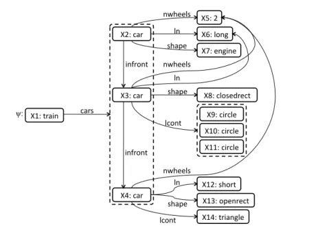
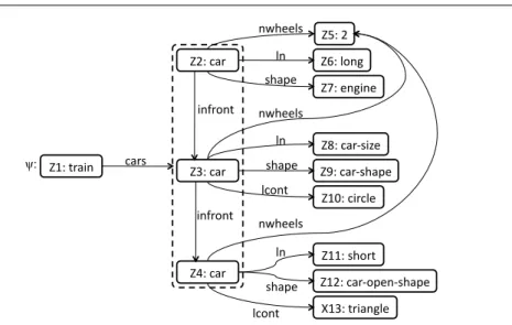
For instance, Figure 2 represents the first west-bound train from Figure 1 using a graphical representation of a feature term. Such train (X1) is composed of three cars (X2,X3andX4), the first of which (X2) is a long engine car with 2 wheels, the second (X3) is a long closed rectangle with 2 wheels holding three circles, and the last one (X4) is a short open rectangle with 2 wheels holding one triangle.

Feature terms can be defined by itssignature:Σ=hS,F,≤,Vi. WhereS is a set of sort symbols, which includes⊥(also called “any”) representing the most general sort and>(also called “none”) representing the most specific sort.≤is an order relation

!"#$%&'()$ !*#$+'&$ !,#$+'&$ !-#$+'&$ !.#$*$ !/#$01)2$ !3#$4)2()4$ !5#$+01647&4+%$ !"8#$+(&+04$ !""#$+(&+04$ !9#$+(&+04$ !"*#$6:1&%$ !",#$1;4)&4+%$ !"-#$%&(')204$ +'&6$ ()<&1)%$ ()<&1)%$ )=:4406$ )=:4406$ )=:4406$ 0)$ 0)$ 0)$ 6:';4$ 6:';4$ 6:';4$ 0+1)%$ 0+1)%$ !:

Fig. 2 A graphical depiction of a train represented using the feature terms representation

formalism.

inducing a single inheritance hierarchy among the sorts inS \ >, and where⊥ ≤s≤ > for anys∈ S.F is a set of feature symbols, andVis a set of variable names.

We define a feature termψas:

ψ::=X:s[f1=. Ψ1, ..., fn=. Ψn]

where ψpoints to theroot variableX (that we will note asroot(ψ)),X ∈ V,s∈ S, fi ∈ F, and Ψi might be either another feature termψi, an already defined variable Y ∈ Vor a set{x1, ..., xm}(where elements are feature terms or variables). When the valueΨi of a featurefi is an already defined variable, we say that there is avariable

equality. Moreover, in our formalization of feature terms we impose the restriction that

each element in a set must be different.

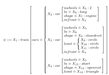
Using this term notation, Figure 3 represents the same train pictured previously in Figure 2, where we can see that the term is composed of 14 variables (corresponding to the 14 nodes in the graphical representation in Figure 2). The term contains two set-valued features (indicated by a curly bracket): in the featurecarsof variableX1, and in the featurelcontof variableX3. Finally, we can also see that there are several variable equalities in this term: since the value of the feature infront of variable X2 is the, already defined, variableX3(we noteX2.inf ront=. X3), and alsoX3.inf ront=. X4. Additionally, the number of wheels in all the cars is the same, and the length of the first two cars is also the same.

In the remainder of this paper we will use vars(ψ) to represent the set of vari-ables in a given feature termψ,f eatures(X) to denote the set of features defined for a variable X, and sort(X) to denote the sort defined for a variable X. Finally, we will define the set reachable(X) as the set of variables reachable from the features of X. For instance reachable(X3) = {X2, X6, X8, X9, X10, X11, X4, X12, X13, X14} and reachable(X14) = ∅. Moreover, if for a particular term ψ there is a variable

ψ::=X1:train 2 6 6 6 6 6 6 6 6 6 6 6 6 6 6 6 6 6 6 6 6 6 6 6 6 6 6 6 4 cars=. 8 > > > > > > > > > > > > > > > > > > > > > > > > > > > < > > > > > > > > > > > > > > > > > > > > > > > > > > > : X2:car 2 6 4 nwheels=. X5: 2 ln=. X6:long shape=. X7:engine inf ront=. X3 3 7 5 X3:car 2 6 6 6 6 6 6 6 4 nwheels=. X5 ln=. X6 shape=. X8:closedrect lcont=. 8 < : X9:circle X10:circle X11:circle inf ront=. X4 3 7 7 7 7 7 7 7 5 X4:car 2 6 4 nwheels=. X5 ln=. X12:short shape=. X13:openrect lcont=. X14:triangle 3 7 5 3 7 7 7 7 7 7 7 7 7 7 7 7 7 7 7 7 7 7 7 7 7 7 7 7 7 7 7 5

Fig. 3 The same train in Figure 2, represented in term notation.

X ∈ vars(ψ) such that X ∈ reachable(X), we will say that ψ has a circular

vari-able equality, or simply acycle.

In our formalization of feature terms, we add the notion of an ontology, which restricts the set of feature terms that can be formed. Thus, in addition to the signa-tureΣ, we will define an ontologyO as a set of restrictions of the form: s1.f $ s2, meaning that any value of a defined featuref∈ F of any variable of sorts1(or more specific) must be of sorts2(or more specific). Moreover, if no restriction appears for a particular featuref for a particular sorts, thenf is not allowed ins. For instance, the ontology for the Trains example would be O ={train.cars $car, train.ncar $ integer, car.inf ront$car, car.nwheels$integer, car.ln$car-size, car.shape$ car-shape, car.lcont$load}. This notion of ontology is a particular case of the full OSF theories presented in [4], but sufficient for the purposes of this paper.

Feature terms can be represented in three different formalisms: they can be repre-sented structurally (as graphs), as depicted in Figure 2, in term notation, as shown in Figure 3, or in clause notation, as shown in Figure 4. The three notations are equivalent, and we will use them indistinguishably in the remainder of this paper. The equivalence between the term form and the clause form is described by A¨ıt-Kaci [4], so that given a term:

ψ::=X:s[f1=. ψ1, ..., fn=. ψn] the clause form can be obtained by a process calleddissolvingas:

φ::=X:s&X.f1=. X1&...&X.fn=. Xn

whereXirepresents the root variable of the termψi. In the case where there is any set-valued featureX.f =. {X1...Xn}, it can be dissolved asX.f =. X1&...&X.f =. Xn. For instance, in Figure 3, the value of the featurecarsof variableX1is a set of three elements (X2, X3, andX4), and thus it is dissolved as X1.cars =. X2 &X1.cars =. X3 &X1.cars=. X4 (as shown in Figure 4).

The basic operation between feature terms issubsumption: we will useψ1vψ2to express that a termψ1subsumes another termψ2– that is to sayψ1is more general (or

φ::=X1:train&X1.cars=. X2 &X1.cars=. X3&X1.cars=. X4&

X2:car&X2.nwheels=. X5&X2.ln=. X6&X2.shape=. X7 &

X2.inf ront=. X3&X5: 2 &X6:long&X7:engine&X3:car&

X3.nwheels=. X5&X3.ln=. X6&X2.shape=. X8 &X3.lcont=. X9 &

X3.lcont=. X10&X3.lcont=. X11&X3.inf ront=. X4&

X8:closedrect&X9:circle&X10:circle&X11:circle&

X4:car&X4.nwheels=. X5&X4.ln=. X12&X4.shape=. X13&

X4.lcont=. X14&X12:short&X13:openrect&X14:triangle

Fig. 4 Representation in clause notation of the train shown in Figure 2.

equal) thanψ21. Another interpretation of subsumption is that of an “informational content” order:ψ1vψ2means that all the information inψ1(all that is true forψ1) is also contained inψ2(is also true forψ2). In our work, we use the definition of sub-sumption introduced in [6] which has a slightly different definition than the traditional θ-subsumption. Specifically, the difference is that we introduce the constraint that all the elements in a set have to be different. See Appendix A for a formal definition.

The subsumption relation induces a partial order in the set of feature terms, i.e. the pairhL,viis aposet for a given set of termsL(called a language); additionally,L contains the infimum element⊥(or “any”), and the supremum element>(or “none”) with respect to the subsumption order. We will work with several languages L of increasing expressiveness, some of which satisfying that hL,vi is a lattice2. In the remainder of this paper we will use G(ψ) = {ψ0 ∈ L|ψ0 v ψ} to denote the set of

subsumersofψin a given languageL, i.e., all the terms which subsumeψ (including

⊥andψitself).

Given the subsumption relation, for any two termsψ1andψ2 we can define their

anti-unification(ψ1uψ2) as theirleast general generalization[36]:

Definition 1 (Anti-unification) Theanti-unification of two terms ψ1 and ψ2, noted asψ1uψ2, is the most specific term that subsumes both:

ψ1uψ2=ψ: (ψvψ1 ∧ ψvψ2)∧(@ψ0Aψ: ψ0 vψ1 ∧ ψ0vψ2)

Anti-unification is relevant for defining similarity measures, since it containsallthe information that is common to bothψ1andψ2. If two terms have nothing in common, thenψ1uψ2=⊥. Thus, anti-unification encapsulates in a single descriptionallthat is shared by two given terms. Additionally, we can generalize the idea of anti-unification to a set of terms, noted by d

({ψ1, ..., ψn}), representing the most specific term that subsumes all the terms in{ψ1, ..., ψn}. Appendix B presents an algorithm to compute one anti-unification of a given set of terms (the algorithm is not specific to feature terms, but can be applied to any representation formalism for which an adequate refinement operator can be defined). A complementary operation to the anti-unification is that of

unification, ormost general specialization:

1 _{Notice that in the description logics notation, subsumption is written in the reverse order}

since it is seen as “set inclusion” of their interpretations. In machine learning terms,AvB means thatAis more general thanB, while in description logics it has the opposite meaning.

2 _{Albeit every partial order with supremum and infimum is trivially a lattice, we will reserve}

the name oflattice for those partial ordershL,viwhere we will define a unification and anti-unification that correspond to the meet and join operations of such lattice.

⊥

⊥

ψ

!

ψ

ψ

!

ψ

a)

b)

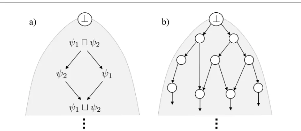
Fig. 5 a) Two termsψ1andψ2and with their unificationψ1tψ2and anti-unification,ψ1uψ2;

b) arefinement graph, where each node represents a term and the most general node is⊥.

Definition 2 (Unification) Theunificationof two termsψ1andψ2, noted asψ1tψ2, is the most general term that is subsumed by both:

ψ1tψ2=ψ: (ψ1vψ ∧ ψ2vψ)∧(@ψ0@ψ: ψ1vψ0 ∧ ψ2vψ0)

When two terms have contradictory information then they have no unifier – which is equivalent to say that their unifier is “none”:ψ1tψ2=>. As before, we can generalize unification to a set of terms, noted byF

({ψ1, ..., ψn}), representing the most general term subsumed by all terms in{ψ1, ..., ψn}.

Figure 5.a graphically illustrates both concepts. Notice that both unification and anti-unification are operations over the subsumption graph: anti-unification corre-sponds to finding the most specific common “parent” (generalization), where as unifi-cation corresponds to finding the most general common “descendant” (specialization). Moreover, unification and anti-unification might be unique or not depending on the structure of the subsumption graph, as we will see later. To simplify the notation, in the remainder of this paper we will assume anti-unification and unification are unique when it does not make a difference.

3 Refinement Graphs for Feature Terms

From the posethL,viwe can derive arefinement graphas the posetR=hL,≺i, where ψ1 ≺ ψ2 represents thatψ2 is aspecialization refinement ofψ1. Conversely,ψ1 is a generalization refinement ofψ2. Formally, the refinement relation used in this paper is defined as:

Definition 3 (Refinement) Two feature terms hold a refinement relationψ1≺ψ2iff ψ1vψ2 ∧ @ψ0:ψ1@ψ0@ψ2

That is to say, the relation ψ1 ≺ ψ2 holds when specializing from ψ1 to ψ2 is a minimal specialization step: there is no intermediate term ψ0 in hL,vi between ψ1 and ψ2. Figure 5.b shows an illustration of the refinement graph, where each node represents a term, and arrows represent refinements. Typically, such refinement graphs have been used in inductive learning and in pattern mining to define the hypothesis

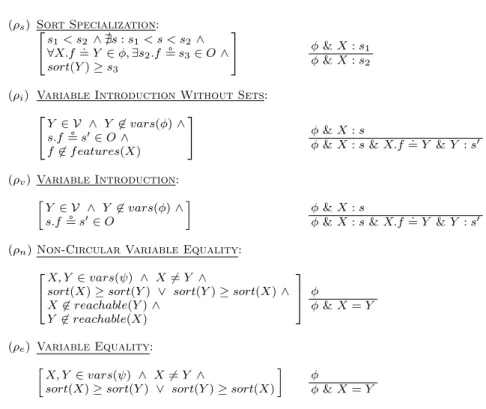
(ρs) Sort Specialization: 2 4 s1< s2 ∧@s:s1< s < s2 ∧ ∀X.f=. Y ∈φ,∃s2.f$s3∈O∧ sort(Y)≥s3 3 5 φ&X:s1 φ&X:s2

(ρi) Variable Introduction Without Sets:

2 4 Y ∈ V ∧ Y 6∈vars(φ)∧ s.f$s0∈O∧ f6∈f eatures(X) 3 5 φ&X:s

φ&X:s&X.f=. Y &Y :s0

(ρv)Variable Introduction: » Y ∈ V ∧ Y 6∈vars(φ)∧ s.f$s0∈O – φ&X:s

φ&X:s&X.f=. Y &Y :s0

(ρn)Non-Circular Variable Equality:

2 6 4

X, Y ∈vars(ψ) ∧ X6=Y ∧

sort(X)≥sort(Y) ∨ sort(Y)≥sort(X)∧ X6∈reachable(Y)∧ Y 6∈reachable(X) 3 7 5 φ φ&X=Y (ρe) Variable Equality: » X, Y ∈vars(ψ) ∧ X6=Y ∧

sort(X)≥sort(Y) ∨ sort(Y)≥sort(X)

– φ

φ&X=Y

Fig. 6 Specialization refinement operators, represented as rewriting rules.

space of inductive learning methods [32]. However, in this paper we will show how to use refinement graphs to define similarity measures.

A refinement graph is defined by arefinement operator, that can be either a

special-ization(ordownward) refinement operator or ageneralization(orupward) refinement

operator. Specifically, a specialization refinement operator is defined as follows:

ρ(ψ) ={ψ0∈ L|ψ≺ψ0}

Whereas a generalization refinement operator is defined as follows:

γ(ψ) ={ψ0∈ L|ψ0≺ψ} Terms are related by refinements paths, as follows:.

Definition 4 (Refinement Path) A finite sequence of terms (ψ1, ..., ψn) is arefinement

pathψ1

ρ

−→ψn between two termsψ1 andψn when for each 1≤i < n,ψi+1∈ρ(ψi). The same definition applies for the generalization refinement operator:ψn−→γ ψ1. This allows us to define a language as follows.

Definition 5 (Language) A language L(for a refinement operator ρ) is the set of termsL={ψ|⊥−→ρ ψ} ∪ {⊥,>}.

ρ

ρ

ρ

ρ

ρ

L

L

L

L

L

L

L

L

Lc

L

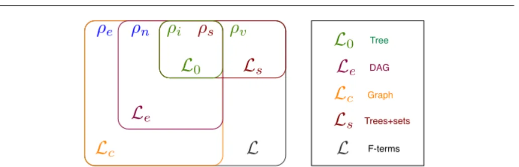
Fig. 7 Different sublanguages of feature terms generated by different subsets of refinement

operators.

That is to say, a language is the set of all termsψ that are reachable from⊥with a refinement path using a particular specialization refinement operatorρ, plus⊥and>. The refinement graphRmight be more or less complex depending on the repre-sentation language being used. For instance, unification and anti-unification might be unique or not. Since the complexity of the refinement graph determines the computa-tional cost of operations defined over it, it is useful to define several languages (different sets of termsL) of feature terms with different expressive power, clearly delineating the areas in which, for instance, the unification is unique (andR=hL,≺iis a lattice). In order to define languages of different expressiveness we will specify several dif-ferent refinement operators. The collection of specialization refinement operators for feature terms are outlined in Figure 6 as rewriting rules. A rewriting rule is composed of three parts: a top part, with the clause representation of a term, a lower part which represents the refinement of that term, and the applicability conditions of the rewrite rule (shown between square brackets in the left hand side of the definition).

Let us briefly review each operator:

– ρs generates refinements by substituting the sort s1 of a variable in a term by a more specific sorts2. Notice that the applicability condition ensures thats1 is substituted only by a direct descendant sort s2 (i.e. @s ∈ S:s1< s < s2) while

satisfying the restrictions in the ontology.

– ρigenerates refinements by adding a feature and its value to a term that previously didn’t have that feature.

– ρvgenerates refinements by adding a value to a feature: if the feature was undefined the operator will add the feature and its value or (if the feature was already defined) add a value to the a set of values of that feature.

– ρngenerates refinements by adding a non-circular variable equality.

– ρegenerates refinements by adding a variable equality (either circular or non cir-cular).

Moreover, notice that all the refinement operators always generate terms that sat-isfy the given ontologyO. Using these refinement operators we will define five languages of increasing expressiveness. Figure 7 shows the relationship between these languages, where set inclusion among languages means thatL ⊂ L0. Let us briefly review them:

– L0is defined by the refinement operators{ρs, ρi}3shown in Figure 6.L0contains all the feature terms that do not have any set-valued feature or any variable equality.

3 _{Notice that in Definition 5 we defined a language from a single refinement operator, and}

Unification and anti-unification are unique inL0. Using the graphical representation of feature terms, the terms inL0are always trees.

– Le is defined by the refinement operators {ρs, ρi, ρn}. Le is a super set of L0 corresponding to all the terms that do not have any set-valued feature or any circular variable equality (non-circular variable equalities are allowed). Unification and anti-unification are also unique. Terms inLeare always DAGs (directed acyclic graphs).

– Lcis defined by the refinement operators{ρs, ρi, ρe}.Lcis a super set ofLewhich allows terms with circular variable equalities. Both unification and anti-unification are still unique. One difference of this language with respect toL0andLeis that some terms might have an infinite number of subsumers, i.e.G(ψ) might be infinite for someψ∈ Lc (see Appendix C).

– Ls is defined by the refinement operators {ρs, ρv}. Ls is a super set of the base languageL0 which allows set-valued features. This language has non-unique unifi-cation or anti-unifiunifi-cation, but all terms have a finite number of subsumers. – L is defined by the refinement operators {ρs, ρv, ρe}. L is a superset of all the

previous languages and contains all feature terms as defined in Section 2. L has non-unique unification and anti-unification, and also some terms might have an infinite number of subsumers.

Notice that the three languages on left part of Figure 7 (L0,Le and Lc) form a lattice with respect the refinement order relation (≺) and have unique unification and anti-unification operations. The other two languages (Lsand L) are just posets with respect to refinement order relation (≺) —since unification and anti-unification may be non-unique when set-valued features are allowed [37].

Refinement operators may be characterized according to three properties:

com-pleteness, properness andlocal finiteness [44]. Completeness states that there are no

refinements of a term which are not generated by the operator, properness means that a term is not equivalent to any of its refinements, and local finiteness means that the number of refinements generated for any given term by the refinement operator is fi-nite. The set of refinement operators {ρs, ρv, ρe} for feature terms presented here is complete, finite and proper4. Notice that for other refinement graphs (such as the ones defined for description logics [29] or the ones defined byθ-subsumption [44]) complete, finite and proper refinement operators do not exist5.

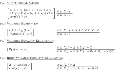
Figure 8 presents the generalization operators for feature terms. Notice that the generalization operators are the same regardless of the language of feature terms used. Nevertheless, depending of the language used, the operators will be complete or not. Concerning the generalization operator, it is not possible to define a complete and still locally finite operator when there are circular variable equalities (see Appendix C). However, for the purposes of this paper (similarity assessment among terms), it suffices with generalization operators that ensure that⊥is reachable by generalizing any term. The operators shown in Figure 8 do ensure that⊥is reached, but they are not complete. Specifically:

operatorsRis equivalent to a single refinement operatorρwhich generates the union of all the refinements generated by the operators inR.

4 _{The operatorsρ}

nandρeshown in Figure 6 are a simplification that might generate some terms that are not refinements, but it’s easy to filter those out using subsumption tests.

5 _{The conditions identified by van der Laag and Nienhuys-Cheng [44] for proving the}

(γs)Sort Generalization: 2 4 s1< s ∧ @s2: s1< s2< s∧ ∀X.f=. Y ∈φ∃s1.f$s3∈O∧ sort(Y)≥s3 3 5 φ&X:s φ&X:s1 (γv)Variable Elimination: » s.f$s0_∈O∧ f eatures(Y) =∅ –

φ&X:s&X.f=. Y &Y :s0

φ&X:s

(γe)Variable Equality Elimination:

ˆ

Z16∈vars(φ)˜ φ&X.f

.

=Z&Y.f0₌. _Z

φ&X.f=. Z&Y.f0=. Z1&Z1:sort(Z)

(γr)Root Variable Equality Elimination:

»

Z16∈vars(φ)∧

root(ψ) =Z –

φ&X.f=. Z

φ&X.f=. Z1&Z1:sort(Z)

Fig. 8 Generalization operators for feature terms. Notice that this operators are not complete,

but that they ensure reaching⊥from any feature term in the language.

– γsgeneralizes terms by substituting the sort of one of the variables in the term by a more general sort.

– γvgeneralizes a term by removing the value of one of the features in one variable of the term. Notice that the operator only removes a variableY iff eatures(Y) =∅, i.e. ifY has no defined features.

– γe and γr generalize a term by removing a variable equality. A circular variable equality can be removed in an infinite number of ways (see Appendix C), and this is the cause of the generalization operators not being complete, although they still ensure that⊥can be reached from any term.

This section has defined refinement operators for feature terms. Nevertheless, the techniques presented in the remainder of this paper are applicable to any other repre-sentation formalism for which (1) a complete and locally finite specialization refinement operator can be defined, and (2) there is a generalization operator that ensures that the most general term (⊥) can be reached from any term through a finite number of steps.

4 Anti-Unification-based Similarity

The anti-unification of two feature termsψ1uψ2is commonly described as their least general generalization. But it is also a symbolic representation of that which is shared

byψ1 and ψ2 and all that is shared. For this reason, anti-unification has been used

in case-based reasoning (CBR) as a form of symbolic similitude [34]. Although this symbolic similitude can be used for explanatory purposes in CBR, another important issue, that we want to address here, is how to quantitatively measure the similarity.

⊥ ψ1 ψ2 ψ1�ψ2 λs λ1 λ2 Sλ(ψ1, ψ2) = λs λs+λ1+λ2

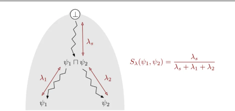
Fig. 9 Illustration of the anti-unification based similarity for two feature termsψ1andψ2

AlgorithmΛ(ψa, ψb, ρ) ForEach (ψ∈ρ(ct) ) Do If (ψvψb∧ψ6vψa) Then ReturnΛ(ψ, ψb, ρ) + 1 EndForEach Return 0 EndAlgorithm

Fig. 10 Given two terms ψa andψb, such that ψa vψb, and a refinement operatorρ, the

algorithmΛreturns the length of the refinement path fromψatoψbin the refinement graph defined by the operatorρ.

That is to say, answering the question “How large isψ1uψ2” might give us a measure that estimates how similarψ1andψ2 are.

Our proposal is to estimate theinformational contentofψ1uψ2, since the larger ψ1uψ2is the more similarψ1andψ2are. The refinement graph gives us a direct way to estimate the informational content of any termψin a languageL: it is the length of the minimal path of refinements that leads from⊥(the most general feature term) toψ itself. In other words, the number of times that a refinement operator has to be applied, starting from⊥, to reachψ. The intuition here is that every time a term is specialized, an extra piece of information is added to it. Using Definition 4 (ofrefinement path) we can characterize any termψ by the path⊥−→ρ ψ, i.e. the refinement path from⊥to ψ; moreover, an estimation of the informational content of any termψis given by the length (λ) of that path:λψ=λ(⊥

ρ −→ψ).

Therfore, the length λ(⊥−→ρ ψ1uψ2) of the refinement path from ⊥to ψ1uψ2 estimates the informational content of that which is common toψ1andψ2(this length is calledλs in Figure 9). In order to define a similarity measure we need to compare what is common to ψ1and ψ2with that which is not. The information in ψ1 that is not common to both terms is exactly what is added by the pathψ1uψ2

ρ

−→ψ1(whose length is calledλ1in Figure 9); and equivalently forψ2with pathψ1uψ2

ρ

−→ψ2(whose length is calledλ2 in Figure 9).

Definition 6 (Anti-unification-based similarity) The anti-unification-based similarity Sλ between two termsψ1andψ2is:

Sλ(ψ1, ψ2) =

λ(⊥−→ρ ψ1uψ2)

!"#$%&'()$ !*#$+'&$ !,#$+'&$ !-#$+'&$ !.#$/0)1$ !2#$3)1()3$ !4#$+'&56(73$ !8#$+'&569':3$ !";#$+(&+/3$ !""#$690&%$ !"*#$+'&50:3)569':3$ <",#$%&(')1/3$ +'&6$ ()=&0)%$ ()=&0)%$ )>933/6$ )>933/6$ )>933/6$ /)$ /)$ /)$ 69':3$ 69':3$ 69':3$ /+0)%$ /+0)%$ !: !?#$*$

Fig. 11 Anti-unification of the two first west-bound trains.

The measure Sλ estimates the ratio between the amount of shared information and the total informational content (i.e. the shared plus the non-shared information). The numerator estimates the shared informational content asλs=λ(⊥−→ρ ψ1uψ2), while the denominator estimates the total amount of information ofψ1and ψ2together by adding the shared informational contentλswith the informational content ofψ1that is not sharedλ1=λ(ψ1uψ2−→ρ ψ1) and the informational content ofψ2 that is not sharedλ2=λ(ψ1uψ2

ρ −→ψ2).

S_λ(ψ1, ψ2) requires computing two things: the anti-unification ψ1uψ2, and the three lengthsλs,λ1,λ2. Appendix B describes an anti-unification algorithm that starts with ⊥ and proceeds by iteratively applying refinement until the anti-unification is reached, returning the anti-unifierψ1uψ2and the length of the refinement pathλs.

The other two lengths (λ1andλ2) are computed by the algorithmΛshown in Figure 10:Λtakes two terms ψa and ψb (such thatψa vψb) and a refinement operator ρ, and returns the number of specialization refinements required to go fromψa to ψb. Therefore, the two lengths can be computed asλ1 = Λ(ψ1uψ2, ψ1, ρ) and λ2 = Λ(ψ1uψ2, ψ2, ρ) whereρis the refinement operator for the language being used.

4.1 Exemplification

To illustrate the anti-unification-based similarity, let us walk through the process of computing the similarity between the first two west bound trains in Michalski’s data set (Figure 1), which we will call ψ6 and ψ7. In order to represent this (apparently simple) data set, the full language L is required. The anti-unification of those two trains (ψ6uψ7) is shown in Figure 11, clearly capturing the key similarities among the two trains: both of them have 3 cars in common, the first car is the engine, which is long and has 2 wheels; both of them have a second car with 2 wheels and which contains at least one circle; and both of them have a third car, which is short, has two wheels, has at least one triangle, and has an open shape (one has an open rectangle shape and the other one has aUshape).

This anti-unification can be computed using the algorithm presented in Appendix B, that also yields the length of the refinement path from⊥toψ6uψ7, which in this case isλs= 40. Then, the algorithmΛin Figure 10 counts the refinement path length from ψ6uψ7 to ψ6, which is λ1 = 8, and from ψ6uψ7 to ψ7, which is λ2 = 19. Notice that the length fromψ6uψ7to the first westbound train is very small (only 8 refinements), while the length to the second westbound train is larger (19 refinements), since the second train has more non-shared content (4 cars, instead of 3).

Thus, the similarity between these two trains is: Sλ(ψ6, ψ7) = 40+8+1940 = 0.597. The interpretation of S_λ is that the ratio 40/67 estimates that these two train de-scriptions share almost 60% of the total informational content. Moreover, thesymbolic

similitude (shown in Figure 11) is capable of conveying an explanation of that which

is behind the numerical similarity value 0.597.

4.2 Discussion

The requirement forSλ to be applied to a refinement graph is that the specialization refinement operators are locally finite and complete. Thus, the anti-unification-based similarity can be applied to any other representation formalisms such that a refinement graph can be defined with a subsumption relation that is compatible with the definition of specialization refinement operators satisfying this requirement.

There are two main issues concerning Sλ worth discussing. The first one is the computational cost of Sλ. Although computing the anti-unification of two terms re-quires (using the algorithm described in Appendix B) a linear number of subsumption tests in function of the size of the terms, testing for subsumption might have a differ-ent computational cost depending on the represdiffer-entation language used. In expressive languages, likeLsand L, subsumption has a higher computational cost than in less expressive languages, such asL0,Le, orLc.

Moreover, in languages where anti-unification might not be unique (Ls and L), ensuring that the maximum similarity value for similarity Sλ is found would involve computing all possible anti-unificationsψ1uψ2 and taking the one that maximizes Definition 6. Computing only one anti-unification (which is the approach taken in the experiments reported in Section 7) results only in an estimation of Sλ that is not ensured to be maximal. Thus, in domains where the instances are large structures and where the language used is very expressive, this trade-off (non-maximal but efficient) may be useful.

A second issue is that Sλ considers each refinement in the refinement graph as equally important; in general, assuming that all pieces of information generated from refinement operators have the same usefulness might not hold. Thus, being able to determine a different weight or importance degree for each of the refinements in the similarity computation is a significant issue that we address on Section 6.

Nevertheless,S_λhas two main advantages: first of all,S_λis a conceptually intuitive similarity measure, and second, during the computation of Sλ a symbolic similitude term is also computed: the anti-unification term ψ1uψ2. As argued by Plaza [35], such term describes in what aspects two instances are similar, and can be used for explanation purposes in Case-based Reasoning systems and other systems estimating similarity among complex descriptions. Additionally the anti-unification term can also be used for case adaptation purposes in CBR (since it makes the similarities between a problem and the retrieved case explicit [12]).

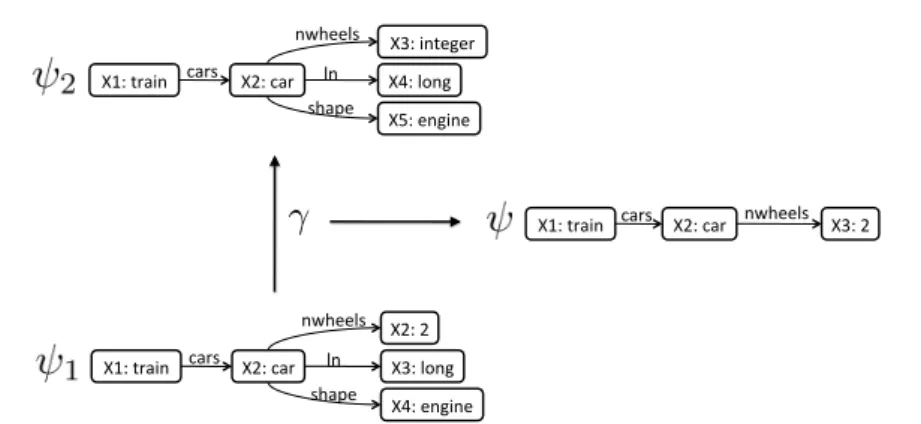
X1:$train$ X2:$car$ X2:$2$ X3:$long$ X4:$engine$ cars$ nwheels$ ln$ shape$ X1:$train$ X2:$car$ X3:$integer$ X4:$long$ X5:$engine$ cars$ nwheels$ ln$ shape$

X1:$train$ cars$ X2:$car$ nwheels$ X3:$2$

Fig. 12 A refinement operatorγthat generalizesψ1intoψ2by subtracting a piece of

infor-mationψcalled theremainderof the refinement.

5 Property-based Similarity

This section introduces the property-based similarity, a new approach to assess simi-larity that is also based on the idea that every specialization refinement adds a piece of informational content to a description (and, conversely, every generalization refine-ment subtracts a piece of informational content from a description), but addresses the two issues ofSλ mentioned above. These pieces of information added or removed by a refinement operator are calledproperties, i.e. a property is some condition that some terms satisfy and some do not. For example, in the Trains domain introduced before, a property might be that “a train has 3 cars”, and some trains might satisfy it while some others might not.

The core idea of the property-based similarity is to disintegrate a term into a collection of smaller terms, which we call properties, and then count how many of those properties they share. Furthermore, we will show it is feasible tointegratethose properties again in order to reconstruct the original term, so no information is lost.

There are several issues that we have to address to define the property-based sim-ilarity. First we will define what constitutes a property; second, we will specify how to disintegrate a term into a collection of properties; and finally, we will define a measure of similarity based on the properties of two disintegrated terms.

5.1 Disintegrating a Term into Properties

Intuitively we would like a property to capture an individual piece of information contained in a term. For instance, in the Trains example used previously, the fact that a train has 4 cars, or that one of the cars is carrying a triangle, are examples of two properties. Generalization refinement operators generate refinements by subtracting pieces of information from terms, and thus making them more general. These pieces of information that are subtracted from terms when generalizing are properties, and will be represented also as feature terms. Dually, specialization refinement operators add pieces of information (properties) to terms. In order to formally define the properties of a term, we will first define theremainderof a generalization refinement operator.

Algorithm Disintegrate(ψ,γ) D=∅, t= 0, ψ0=ψ While (ψt6=⊥) Do ψt+1∈γ(ψt) D=D∪ {r(ψt, ψt+1)} t=t+ 1 EndWhile ReturnD EndAlgorithm

Fig. 13 Algorithm to disintegrate a termψinto a property setD(ψ).

Definition 7 (Remainder) Given a term ψ2 ∈ γ(ψ1), where γ is a generalization refinement, theremainderr(ψ1, ψ2) of such generalization is a term ψsuch thatψt ψ2=ψ1and@ψ0∈G(ψ1) such thatψ0@ψandψ0tψ2=ψ1.

That is to say, the remainder of a generalizing refinement γ from ψ1 to ψ2 is the most general termψ such that when unified with the generalizationψ2 obtains back the original termψ1. We will call this remainderψaproperty of ψ1. Notice that the remainder is the most general term that captures which is the “property” thatψ1 has and that is not present in ψ2, i.e. the informational content that the generalization operator removed. Figure 12 illustrates this idea, where a train is generalized with a refinement operator, and the property subtracted is the fact that the car of that train has 2 wheels. The remainder of a specialization refinementρcan be defined similarly.

Now, if we iterate this generalization refinement over the resulting term and keep generalizing it, we will obtain a collection of properties as remainders of each step. In the end, the iterative generalization process will reach⊥, the empty term, and we will have a collection of properties satisfied by the initial term. This is the intuitive idea

ofterm disintegration: generalize a term repeatedly until reaching⊥while collecting a

property at each step by getting the remainder of the generalization operation. Definition 8 (Disintegration) Given a finite refinement pathp=ψ1

γ

−→ ⊥consisting of a sequence of terms (ψ1, ..., ψn=⊥), adisintegrationof a termψ1is the setDp(ψ1) = {r(ψi, ψi+i)|1≤i < n},

That is to say,Dp(ψ1) is the set of remainders resulting from each generalization step inpfromψ1 to⊥.

Given a refinement path ψ −→ ⊥γ , and having in mind that refinement operators represent the most fine-grained steps in which terms can be specialized or generalized, the remainders obtained from such paths correspond to the most primitive pieces of information contained in a termψ. Therefore, the disintegration of a term is a process that breaks up a term into its most constituent and primitive pieces of information (with respect to a particular language); each one of these pieces of information is also represented as a term, and is what we call aproperty.

Figure 13 presents an algorithm to compute the disintegration of a termψ. Given a termψ, and a generalization refinement operatorγ, the algorithm proceeds iteratively, generalizing ψ using γ, until ⊥ is reached. At each iteration t of the algorithm, a new generalizationψt+1 is generated by taking one of the generalizations (it does not matter which one) generated byγfrom the current termψt. Then, the property setD is expanded by adding the remainderr(ψt, ψt+1) of generalizingψtinto ψt+1. When ⊥is reached, the algorithm returns the setDcontaining all the properties generated so far, corresponding to a disintegration of the termψ.

X2:car X4:long X5:engine shape ln X1:train X3:car X6:short X7:openhex cars ln shape infront

Y1:train cars Y2:car shape Y3:engine

cars

h ln

Y1:train cars Y2:car infront Y3:car shape Y4:car‐shape l d h

cars infront _Y3 shape

Y1:train cars Y2:car

Y2:car Y4:short ln

Y1:train cars Y2:car infront Y3:car ln Y4:car‐length Y1:train cars Y2:car Y3:car p Y4:closed‐shape

Y1:train

Y2:car

Y3:car

cars Y4:ccar‐shape shape

Y5:short ln

Y1:train cars Y2:car ln Y3:long

Y1:train

Y2:car

Y3:car cars

infront

Y2:car ln Y3:car length

Y1:train

Y2:car

Y3:car cars

Y1:train cars Y2:car Y1:train cars Y3:car shape Y3:openhex

Y1:train

Y2:car

Y3:car

cars Y3:car‐length Y3:car‐length ln

Y1:train Y2:car

Y1:train Y1:train cars Y2:car infront Y3:car shape Y4:open‐shape

Fig. 14 An example feature term disintegrated into properties using the algorithm in Figure

13.

Theintegration of a property set is the process opposite to disintegration, and is

defined asintegrate(D(ψ)) =F

(D(ψ)), that is to say the unification of all properties of a disintegrated term ψ. Integrating a disintegrated term allows as to recover the original term, as shown in the following Lemma.

Lemma 1 One of the unifications of all the properties of a termψis exactly the term

ψ, i.e.ψ∈F

(D(ψ)). When unification is unique, thenψ=F

(D(ψ)).

Proof Letψ1be a term that when disintegrated using the refinement path (ψ1, ..., ψn=

⊥) yields the properties (r1, ... ,rn−1). Definition 7 (Remainder) ensures thatψi+1t ri=ψi(or thatψiis one of the unifications ifψi+1triis not unique). Let us consider first the case when unification is unique. Iteratively unifying the properties in the reverse order in which they were generated, we can reconstruct the refinement path: ψn−1=rn−1,ψn−2=rn−1trn−2,ψn−3= (rn−1trn−2)trn−3, etc. Thus,ψ1 =

F

i=n−1...1ri, which is preciselyF(D(ψ)). When unification is not unique, we know by Definition 7 that:ψn−1=rn−1,ψn−2∈rn−1trn−2,ψn−3∈(rn−1trn−2)trn−3, etc. Thus,ψ1∈F

i=n−1...1ri, which is preciselyF(D(ψ)).

Figure 14 shows an example of the disintegration process, where a simple train represented as a feature term (top half) has been disintegrated into properties (bottom half). Disintegration extracted 14 properties from this train, since the refinement path used had 14 generalization steps. Also, notice that different refinement paths might generate different disintegrations; Section 5.3 discusses this and other properties of the disintegration operation within the different languagesLwe have defined. But let us first present the formal definition of the property-based similarity.

5.2 Property-based Similarity Measure

Theproperty-based similarity Sπ of two termsψ1andψ2uses disintegration to obtain

their their property sets D(ψ1) and D(ψ2) and compares how many properties are shared and how many are not.

Definition 9 (Property-based Similarity Measure) Sπ(ψ1, ψ2) =|D(ψ1)∩D(ψ2)|

|D(ψ1)∪D(ψ2)|

That is to say, Sπ is the ratio between number of shared properties, and the total number of properties that at least one of the two terms satisfies. An equality among feature terms is required in order to perform set intersection and union of property sets, which we define in the usual way:ψ≡ψ0 ⇐⇒ (ψvψ0∧ψ0vψ).

Notice that in the disintegration process each property corresponds to one refine-ment. Therefore,Sπshould provide results similar to those ofSλ, since each refinement in the path⊥−→ρ ψ1uψ2corresponds to a shared property inSπ(see Section 5.3 below). The advantage of the property-based similaritySπis that its computational cost is lower than that ofSλ. For data sets with complex cases, computing the anti-unification of two terms (as required by Sλ) might be very costly, while properties can be ex-tracted at a reasonable cost. Although the formal analysis of computational complex-ity of both similarcomplex-ity measures is outside the scope of this paper, Section 7 shows an empirical evaluation of their average computational cost. Intuitively, the idea be-hind the property-based similarity is to go from unification and anti-unification of terms to union and intersection of properties. This is a powerful idea, since unifica-tion and anti-unificaunifica-tion are expensive operaunifica-tions, while union and intersecunifica-tion are cheaper; the only cost is associated with subsumption for computing term equality, since ψ1≡ψ2 ⇐⇒ (ψ1 vψ2∧ψ2 vψ1). Subsumption among properties is a fast and efficient operation in practice, as long as we are in a domain where properties are represented by small-sized terms.

Finally, the requirements forSπ(and the disintegration operation) to be applied to a refinement graph are: (1) there is a unification operation, and (2) the generalization refinement operators ensure that for everyψthere is a pathψ−→ ⊥γ .

5.3 Disintegration and Feature Term Languages

Depending on the refinement path used for disintegration and on the language used, we might obtain different property sets. Specifically, depending on the language being used, term disintegration following Definition 8 can be eitherweaklyorstrongly complete. Definition 10 (Weak Completeness) Disintegration isweakly complete, when, given any term ψ, we have that ψ ∈ F

(D(ψ)) —i.e. integrating all the properties using unification recovers the original termψ.

For a given termψ, the property setD(ψ) obtained by the disintegration algorithm in Figure 13 is always at least weakly complete since (as shown in Lemma 1)ψ∈F

(D(ψ)). Definition 11 (Strong Completeness) Disintegration isstrongly completewhen, given any two termsψ1 and ψ2, we have thatψ1uψ2 ⊆F(D(ψ1)∩D(ψ2)) – integrating the properties common to both disintegrations recovers the anti-unification of the two terms,ψ1uψ2.

ψ

ψ

ψ

t

ψ

ψ

u

ψ

D

(

ψ

)

∩

D

(

ψ

)

D

(

ψ

)

∪

D

(

ψ

)

D

(

ψ

)

D

(

ψ

)

Fig. 15 Disintegration maps a termψinto a property setD(ψ) allows to go from unification

and anti-unification of terms (on the right side) to union and intersection of properties (to the left side), which are computationally cheaper. Thus, the term resulting from integrating the intersection of the properties of two terms is an approximation of its anti-unification.

Notice that strong completeness implies that given any pair of termsψandψ0such that ψ0vψ, there is a subset of propertiesD0⊆D(ψ) such thatψ0∈F

(D0), i.e. any term which is a subsumer ofψcan be generated as the unification of a subset of properties of ψ. This is because ifψ0 vψ then ψuψ0 =ψ0, and thusψ0 ∈ F

(D(ψ)∩D(ψ0)); moreover,D0=D(ψ)∩D(ψ0).

Disintegration is strongly complete in the languageL0. The reason is that, regard-less of which refinement path is used, the property set obtained is the same —the properties are just obtained in a different order (this is a direct implication of terms in L0 being always trees). Given two terms, ψ1 and ψ2, we can always find refine-ment paths fromψ1 to⊥and fromψ2 to⊥that traverse their anti-unification term ψa = ψ1uψ2. Therefore, the set of properties generated for ψ1 or for ψ2 by disin-tegration using those paths will contain the set of properties ofψa. Since, regardless of the path, we obtain the same property sets, the disintegrations ofψ1 andψ2 each contain all the properties of ψa, and thus the unification of the intersection of their property sets is exactlyψa. Additionally, there is a more efficient algorithm to obtain the remainders inL0 [33].

If we move to more expressive languages likeLsandLe, the property set generated will be different depending on the refinement path used to disintegrate a term, and the disintegration operation cannot be guaranteed to be strongly complete. New ways of disintegrating terms are part of our future work. Additionally, studying whether different refinement paths for disintegration affectsSπ, in the sense that some might be more efficient or accurate, is also part of our future work.

Finally, disintegration can never be strongly complete in languagesLc andL, even if other disintegration algorithms are devised. The reason is that, since they allow cyclic variable equalities, the set G(ψ) of some ψ might be infinite (see Appendix C). For having strong completeness, we need to have a subset of properties inD(ψ) which can recover every term in G(ψ), i.e. there is a mapping between the parts ofD(ψ) and elements ofG(ψ). SinceD(ψ) is finite, it is not possible to find such mapping when G(ψ) is infinite.

5.4 Approximation ofSλ bySπ

We will now show thatSπ approximatesSλ. The difference between the two is work-ing with unification and anti-unification between terms versus workwork-ing with union and intersection of properties, as shown in Figure 15. In fact, they are equal when disinte-gration is strongly complete, i.e. for languageL0, whereSλ=Sπ, because (as we saw) property sets are unique and thusψ1uψ2=F

(D(ψ1)∩D(ψ2)). The approximation is partial for more complex languages for which disintegration is not strongly complete. That is to say, we cannot ensure thatψ1uψ2is equal toF(D(ψ1)∩D(ψ2)).

When disintegration is weakly complete, the term resulting from unification of the shared properties might be more general than the anti-unification of the terms. Lemma 2 The unification of all the shared properties of two termsψ1andψ2is always

more general or equal to their anti-unification, i.e.

∀ψ∈G(D(ψ1)∩D(ψ2)),∃ψa∈ψ1uψ2:ψvψa

Proof The proof is a straightforward implication of the definition of unification and

anti-unification. All the properties in D(ψ1)∩D(ψ2) subsume both ψ1 and ψ2, and thus they must also subsume at leas one of their anti-unification(s), i.e.∀ψ∈D(ψ1)∩ D(ψ2) :ψvψa(for someψa∈ψ1uψ2) – see Definition 1. Therefore, by Definition 2,

F

(D(ψ1)∩D(ψ2))vψa.

Notice that the term resulting from unification of the shared properties might be more general than the anti-unification of the terms when disintegration is weakly complete, since there might be some properties shared byψ1 and ψ2 that are not in their disintegrations.

As a consequence,Sπ is an underestimator ofSλ(Sπ≤Sλ), assuming the refine-ment paths used in both similarities are the same. The reason is that, in Definitions 6 and 9, the numerator in Sλ is greater or equal to the numerator in Sπ, and the denominator in Sλ is lower or equal to the denominator in Sπ. First, notice that |D(ψ1)| = λs+λ1 and |D(ψ2)| = λs+λ2, since the number of properties in the disintegration of the terms is identical to the lengths of the refinement paths used to disintegrate them. However, |D(ψ1)∩D(ψ2)| ≤ λs since, even when the paths are the same, the set of properties may be different, and there are some properties shared by ψ1 and ψ2 that are not in both of their disintegrations. Consequently, the nu-meratorSλ is greater or equal to the numerator inSπ and the denominator satisfies |D(ψ1)∪D(ψ2)|=|D(ψ1)|+|D(ψ2)| − |D(ψ1)∩D(ψ2)| ≥ |D(ψ1)|+|D(ψ2)| −λs= λs+λ1+λ2.

6 Weighted Property-based Similarity

Since each property represents a piece of information,Sπ measures how many pieces of information are shared among two given terms. However, when using this similarity measure for a particular learning task, not all the pieces of information shared among two terms might be equally important.

An interesting advantage of the property-based similarity is that we can assess the importance of each individual property for the task at hand and thus determine a weight for each property. For classification tasks, assume our training set isT = (c1, . . . , cn)

Data set Examples Classes Variables Sets Properties L Soybean 307 18 8 - 38 0 12 - 72 L0 Demospongiae-280 280 3 20 - 48 0 - 18 32 - 106 Ls Demospongiae-503 503 8 20 - 51 0 - 18 32 - 106 Ls Trains 10 2 14 - 23 3 - 6 46 - 78 L Kinship 24 2 14 0 - 8 67 - 110 L PTC-MR 297 2 6 - 138 0 - 64 7 - 523 L PTC-FR 296 2 6 - 138 0 - 76 7 - 491 L PTC-MM 296 2 5 - 138 0 - 76 7 - 523 L PTC-FM 319 2 5 - 138 0 - 76 7 - 523 L

Table 1 Data set size and complexity comparison, showing the number of examples and classes

of each data set, the ranges in number of variables and set-values features in the examples, the ranges in number of properties produced by disintegration of examples, and the language Lused to represent the data set.

and an example is a pair ci = (pi, si), i.e. a problem description pi and a solution classsi. In order to asses property weights, we takeT’s problem descriptions (pi) and disintegrate them obtainingD(pi) for each example inT. Then, theproperty dictionary D(T) of the training setT is obtained by the set of all (non-equivalent) properties of the examples, i.e.D(T) =S

i=1,...,nD(pi).

The second step is to estimate a weight w(ψ) for each propertyψin the property dictionaryD(T). Each propertyψdivides the set of training instances in two sets:Tψ andTψ, whereTψ={ci∈T|ψ∈D(pi)}is the subset of examples that satisfy a given propertyψandTψ={ci∈T|ψ6∈D(pi)}is the subset of those that don’t. A measure such as Quinlan’s Information Gain [38] can be used to compute property weights. The following equation determines the weight of each propertyψ∈D(T) using Information Gain:

w(ψ) =H(T)−H(Tψ)× |Tψ|+H(Tψ)× |Tψ| |T|

where H(X) represents the entropy of the set of instances X with respect to the partition induced by the solution classes, and |X| is the cardinality of setX. Thus, given thatD(ψ) is the subset of properties D(ψ) ⊂D(T) that a particular term ψ satisfies, the weighted property-based similaritySwπ between two terms is defined as follows:

Definition 12 (Weighted Property Similarity) Swπ(ψ1, ψ2) =

P

ψi∈D(ψ1)∩D(ψ2)w(ψi) P

ψj∈D(ψ1)∪D(ψ2)w(ψj)

That is to say,Swπis the sum of the weights of those properties shared by two termsψ1 andψ2, divided by the sum of the weights of all the properties that at least one of the termsψ1andψ2satisfies. Clearly,Swπis independent of the Information Gain measure, and any other way to estimate importance of properties could be used. Nevertheless, the experiments reported in the next section use Information Gain for estimating the weight of properties.

7 Experimental Evaluation

In order to evaluate our similarity measures, we measured the performance of a nearest neighbor method using them. We used five different data sets:Soybean,Demospongiae,

Trains,KinshipandToxicology(PTC). The different characteristics of these data sets are shown in Table 1. Trains is the data set shown in Figure 1, as presented by Michalski [27]; the full languageLis required to represent this data set. Soybean is a propositional data set (representable usingL0) from the UCI machine learning repository consisting of 307 cases and 18 solution classes.

Kinship is a small but complex relational data set consisting of two families where the goal is to learn family relations likeuncle [22]. Each family has 12 members (thus 24 persons in total); the full language L is required to represent this data set. The representation is purely relational, and each family is a graph (with most features in-troducing circular variable equalities); there are 4 positive examples and 20 negative examples. We selected the Trains and Kinship data sets to highlight domains that are highly relational and where the value of features is not as important as the structure of the terms. The Demospongiae data set is a relational data set from the UCI ma-chine learning repository (with sets, but no variable equalities, and representable in Ls) composed of 503 Demospongiae belonging to 8 different solution classes. For the Demospongiae data set, we report results both using the complete data set as well as using a subset consisting of 280 Demospongiae and 3 solution classes.

Finally, the Toxicology data set (PTC) is a highly relational data set introduced as a challenge in the ECML/PKDD 2001 conference [21]. We have selected PTC to evaluate the scalability of our similarity measures rather than their accuracy; thus, we present results for Toxicology in a separate section. The original dataset consists of a collection of Prolog facts, so, for our evaluation we used the version created by Armengol and Plaza [8], who converted the dataset to feature terms using a chemical ontology and which contains 371 examples. The Toxicology dataset consists of a collection of molecules and the task is to predict their carcinogenicity (positive or negative) for four different types (MR, FR, MM, FM) given by sex (M and F) or species (M and R). For each different type, a different subset of the 371 examples is used, and they are shown in Table 1 as separate data sets.

Additionally, in order to better measure the complexity of each dataset, Table 1 shows some statistics of each data set. Specifically, the first two columns in Table 1 shows the number of examples of each dataset and the number of solution classes. The third column shows the number of variables present in the feature terms representing the examples of each data set; we show the range from minimum to maximum number of variables. The larger the number of variables, the larger the examples – for instance the term in Figure 2 has 14 variables. As Table 1 shows, the larger examples are found in the Toxicology dataset, where some examples have up to 138 variables. The fourth column of Table 1 shows the total number of variables occurring in set-valued features (minimum and maximum); this factor plays an important role in the computational cost of subsumption. The only data set without set-valued features is Soybean. The fifth column shows the number of properties obtained by disintegrating the examples of a dataset: the more properties the more complex the examples are. This number is equivalent to measuring the length of a refinement path from⊥to a given example (i.e. it is a measure of the amount of information contained in each example); we show the minimum and maximum number of properties. Again, this shows that the Toxicology data set has some very large examples, some of them generating up to 523 properties. The last column in Table 1 shows the language required to represent the examples in each data set.

Sλ Sπ Swπ SHAUD RIBL Kashima 1-NN Soybean 91.53 91.53 91.21 91.53 91.53 92.18 Demospongiae-280 95.00 94.64 96.79 95.71 91.67 90.71 Demospongiae-503 89.66 90.26 92.44 88.27 88.93 83.10 Trains 50.00 60.00 60.00 - 50.00 20.00 Kinship 100.00 87.50 100.00 - 83.33 83.33 3-NN Soybean 88.93 89.58 88.27 88.93 88.93 87.95 Demospongiae-280 94.29 95.71 96.79 95.00 91.67 90.71 Demospongiae-503 88.27 90.66 90.46 87.08 86.43 83.10 Trains 60.00 70.00 70.00 - 70.00 30.00 Kinship 91.67 83.33 83.33 - 83.33 83.33

Table 2 Classification accuracy (in percentage) measured using a leave-one-out method for

different similarity measures.

7.1 Classification Accuracy Comparison

Table 2 shows the classification accuracy for several similarity measures in the data sets used for our evaluation —except the PTC data set that is addressed later in Section 7.2. We report results forSλ and for both Sπ andSwπ, as well as two other relational similarity measures (SHAUD [7] and RIBL [17]) and a graph kernel [25] for comparison purposes. For each similarity measure we measured classification accuracy using both 1-nearest neighbor and a 3-nearest neighbor by means of a leave-one-out method. SHAUD is a relational similarity measure defined for feature terms that has been shown to obtain very good results in complex relational data sets, and RIBL is a well known similarity measure for first order logic (FOL). RIBL requires examples to be represented in FOL and not as feature terms, but feature terms can actually be converted to FOL predicates without losing information. We used such conversion to evaluate RIBL.

Moreover, RIBL and SHAUD require knowing the ranges of each numeric feature in order to compute the similarity values. We used the minimum and maximum values observed in the data set to define such ranges. RIBL also requires a maximum depth parameter, that was set to 10 in our experiments. Since SHAUD works only for trees, it could not be applied to the Kinship or Trains data set.

We also used the random-walk graph kernel [25], that we will refer to as Kashima’s kernel. Given two graphs, Kashima’s kernel computes the expected similarity between a random walk from one graph and a random walk from the other graph. This kernel has a low computational cost for acyclic graphs, but requires inverting a matrix with n×mrows andn×mcolumns (wheren andmare the number of nodes of the two graphs) when there are cycles in the graph, and thus it can only be calculated using a numerical approximation. Since Kashima’s kernel works on labelled graphs, we used the graph representation of feature terms. Moreover, Kashima’s kernel has two parameters: γ, that corresponds to the probability of a random walk to end, and a kernel to assess similarity among the labels in the graph. We experimented with different values forγ, and usedγ= 0.1 in our experiments, since it gave the best results overall. We used the sort ontology to define a kernel for the labels of the graph (to ensure that the kernel can exploit all the information available to the other similarity measures).

Table 2 shows the classification accuracy of these methods, with the highest ac-curacy for a given data set shown in bold; most of the times the difference between

the accuracy shown in bold and the rest is statistically significant using a t-test with p <0.05, with the following exceptopns: in the Trains data set (which only has 10 in-stances), in the Demospongiae-503 data set with 3-NN (where the difference betweenSπ andSwπ is not statistically significant), and in the Demospongiae-280 data set, where it is only significant with p <0.25. Table 2 shows that the weighted property-based similarity (Swπ) achieves the highest classification accuracy in all data sets except for Soybean (but where the difference is not statistically significant when using 3-NN). The Soybean data set is a propositional one, where the most important issue is the value of the features, and not the relational structure in the instances; however, Sπ achieves the same classification accuracy as both SHAUD and RIBL, and only slightly under that achieved by Kashima’s kernel.

Structure is the only important factor in the Kinship data set. SHAUD cannot be applied since instances are not trees, and RIBL has problems also, since there are no numerical or symbolic values in any of the terms in Kinship, only a graph relating each member of the family to each other. In fact RIBL achieves an accuracy of 83.33% only because it always predicts “negative”, and there are only 4 positive examples out of 24.Sλ and Swπ are able to capture the structure of the instances, and achieve an accuracy of 100.00% when used in a 1-NN.Sπalso achieves a high accuracy, although not a 100.00%.

Trains is an apparently simple but complex data set, since out of the numerous features in each train only two are key to determine the class, and it is hard to learn this with only 10 instances.Swπand RIBL perform the best in this data set.

In the Demospongiae data set,Swπachieves the best results. SHAUD,Sπ, andSλ achieve also good results but not as good, and finally Kashima’s kernel gets the lowest accuracy. RIBL does not perform well in this data set either, because it does not exploit completely the information in the sort taxonomy, which is important in this data set. Moreover, notice that RIBL can accept weights in both predicates and attributes, but there is no simple way to compute them directly (like with the properties in Swπ), and thus we used uniform weights. Thus, the results reported here for RIBL might be suboptimal, although weights would not allow RIBL to improve in this data set.

Comparing with Kashima’s kernel, Table 2 shows that the kernel achieves good results only in the Soybean dataset. The issue seems to be that Kashima’s kernel simply estimates the similarity among two graphs; for instance, in the Kinship dataset, the graphs representing some of the examples are identical (since all the examples belong to the same family). However, both RIBL and our measuresSπ andSλ consider the similarity among instances that, albeit are graphs, start at a specific node (called the root node in feature terms). To determine whether this was the case, we performed a second set of experiments (not shown on Table 2) where we used Kashima’s kernel, but only considering random walks starting from a root node. Using this second version, we achieved better results in the Trains and Kinship datasets. In the Trains dataset, accuracy went up to 50% for 1-NN and 60% for 3-NN, while in the Kinship dataset, accuracy went up to 87.5% both using 1-NN and 3-NN.

The computational cost of different similarity measures, evaluated as the average execution time to compute the similarity between two instances in different data sets, is shown in Table 3. The most computationally expensive similarity measures areSλand SHAUD, since they perform the anti-unification of the two instances being compared. For instance, in the Demospongiae data set,Sλ takes 66.23 milliseconds6 on average

Sλ Sπ/Swπ SHAUD RIBL Kashima Soybean 66.30ms 0.36ms 23.86ms 1.90ms 1.37ms Demospongiae-280 66.23ms 2.65ms 28.24ms 5.26ms 3.09ms Demospongiae-503 62.72ms 3.17ms 23.00ms 5.25ms 4.36ms Trains 158.35ms 4.29ms - 7.81ms 1.35ms Kinship 85.84ms 5.39ms - 9.69ms 15.87ms

Table 3 Average time (in milliseconds) required to compute the similarity of two instances

for different similarity measures.

Sπ Swπ RIBL 1-NN PTC-MR 57.24 58.59 57.91 PTC-FR 63.04 61.39 66.33 PTC-MM 58.06 60.87 50.83 PTC-FM 62.07 58.62 56.43 3-NN PTC-MR 51.85 57.58 59.59 PTC-FR 56.44 63.37 64.03 PTC-MM 57.19 65.22 56.52 PTC-FM 58.93 60.19 54.23

Table 4 Classification accuracy for PTC in percentage measured using a leave-one-out method

for different similarity measures.

to assess one similarity. SHAUD takes 23.86ms, and the property based similarities Sπ and Swπ take 2.65ms. RIBL is also a fast similarity measure, taking only 5.26 milliseconds per similarity in the Demospongiae data set. Kashima’s kernel is very fast in the Soybean, Demospongiae and Trains data sets, since they do not contain cycles. However, Kashima’s kernel has a much higher computational cost in the Kinship data set (15.87ms), since it contains cycles7.

Computing the weights of properties in Swπ, as well as disintegrating an example into properties, are processes typically performed offline, since they only need to be performed once, and their cost is not included in the time for computing the similarity among 2 instances. Computing weights forSwπin our experiments takes 79.82ms in the Soybean dataset, 389.20ms and 983.92ms in the 280 and Demospongiae-503 data sets, 1.50ms in the Trains data set, and 49.68ms in the Kinship data set. Disintegrating the complete Soybean data set takes 8.12 seconds, the Demospongiae data set requires 328.77 seconds, while the Trains and Kinship data sets take 7.45 and 18.85 seconds respectively.

The next two subsections evaluate the scalability of our similarity measures by using first a data set with very large examples and then a data set with a large number of examples.

7.2 Evaluation with Large Examples

In order to evaluate the scalability of Sλ and Sπ, we selected the Toxicology data set, which contains some very large molecules (with up to 138 variables in the terms representing the examples). SHAUD could not be applied to Toxicology, since molecules

7 _{We used theColtJava matrix library for Kashima’s kernel for high performance matrix}

Sπ/Swπ RIBL PTC-MR 4.05ms 5.85ms

PTC-FR 9.76ms 5.84ms PTC-MM 10.26ms 5.84ms PTC-FM 10.11ms 5.79ms

Table 5 Average time (in milliseconds) required to compute the similarity of two instances

for different similarity measures in the Toxicology data set.

are cyclic graphs (SHAUD was applied to a subset of the Toxicology data set [7], consisting of molecules without cycles when represented as feature terms). Additionally, due to the size of the molecules,Sλ could not be applied to the Toxicology data set, since there is a small set of molecules that are too large for computing anti-unification in a reasonable amount of time.

Table 4 shows the classification accuracy results for the Toxicology data set in its 4 animal groups. RIBL performs well for the MR and FR animals, but rather poorly in MM and FM.SwπoutperformsSπin all tests except in FR and FM using a 1-NN. Using a 3-NN,Swπ always outperformsSπ. The accuracy levels achieved for the Toxicology data set are comparable to the results obtained with other techniques. For instance, using graph-kernels, Kashima et al. [25] report between 54.1% to 58.4% accuracy for MR depending on the value set for the parameterγof their algorithm (the termination probability of random walks). They also report between 62.1% to 66.1% for FR, 62.2% to 64.3% for MM and between 59.3% to 63.4% for FM. Moreover, the maximum and minimum accuracy for each type were achieved with a different value of that parameter. The results obtained withSwπusing a 3-NN are inside or above those ranges, without the need to