Computational Tool for Applications of Sparse Canonical Correlation Analysis on Biological Data

(1)

COMPUTATIONAL TOOL FOR APPLICATIONS OF SPARSE CANONICAL CORRELATION ANALYSIS ON BIOLOGICAL DATA

A Thesis by

RATANOND KOONCHANOK

Submitted to the Office of Graduate and Professional Studies of Texas A&M University

in partial fulfillment of the requirements for the degree of MASTER OF SCIENCE

Chair of Committee, Ulisses Braga-Neto Co-Chair of Committee, Ivan Ivanov

Committee Members, Robert Chapkin Erchin Serpedin Head of Department, Miroslav Begovic

December 2017

Major Subject: Electrical Engineering

(2)

ABSTRACT

Sparse canonical correlation analysis (sparse CCA) is a method for identifying sparse linear combinations of the two sets of variables that are highly correlated with each other, given that those two sets of measurements are available on the same set of observations. Recently, sparse CCA has become a popular method for analyzing genomic data, where the number of features is large compared to that of observations. Analyzing a set of data using sparse CCA requires multiple steps, including data cleaning, normalizing, and using the right programming packages.

To make sparse CCA accessible for all researchers regardless of their statistical background, a user-friendly computational tool should be created to assist them in walking through the analysis. After the tool is successfully implemented, a few sets of data will be used as case studies for testing efficiency of the sparse CCA computational tool. Eventually, the tool will be added to the computational website hosted by the Center for Translational Environmental Health Research, which currently hosts services for sequencing classification and differential expression analysis.

(3)

ACKNOWLEDGEMENTS

I would like to thank my committee chair and co-chair, Dr. Braga-Neto and Dr. Ivanov, for giving me a great opportunity to work on a meaningful project as well as for providing many informative advice throughout the course of this research. I also would like to thank my two committee members, Dr. Chapkin and Dr. Serpedin. They not only joined the thesis defense, but also offered valuable suggestions.

Thanks also go to my friends and colleagues and the department faculty and staff for making my time at Texas A&M University a great experience. Finally, thanks to my parents for their encouragement, patience, and love.

(4)

CONTRIBUTORS AND FUNDING SOURCES

This work was supervised by a thesis committee consisting of Dr. Ulisses Braga-Neto of the Department of Electrical and Computer Engineering (co-advisor), Dr. Ivan Ivanov of the Department of Veterinary Physiology and Pharmacology (co-advisor), Dr. Robert Chapkin of the Department of Nutrition and Food Science and Dr. Erchin Serpedin of the Department of Electrical and Computer Engineering.

All work for the thesis was completed independently by the student.

This work was made possible in part by the National Institutes of Health under Grant Number R35CA197707 and P30ES023512.

(5)

TABLE OF CONTENTS

Page

ABSTRACT... ii

ACKNOWLEDGEMENTS... iii

CONTRIBUTORS AND FUNDING SOURCES... iv

TABLE OF CONTENTS... v

LIST OF FIGURES... vii

LIST OF TABLES... ix

1. INTRODUCTION... 1

2. BACKGROUND... 3

2.1 Canonical correlation analysis (CCA)……….. . 3

2.1.1 CCA………... 3

2.1.2 Sparse CCA………... 3

2.1.3 Important terms………... 4

2.2 Comparison with other types of analysis………... 5

2.2.1 Principal component analysis (PCA)……….... 5

2.2.2 Pearson’s correlation coefficient………... 6

2.3 Probability distribution models for generating synthetic biological data... 7

2.3.1 Multivariate Gaussian distribution……… 7

2.3.2 Poisson distribution………... 8

2.4 Current state of the computational website……….... 10

3. RESEARCH DESCRIPTION……….. 13

3.1 Problem definition………. 13

3.2 Research goals……… 14

4. PROJECT APPROACH... 16

(6)

4.2 Sparse CCA implementation... 18

4.2.1 ‘CCA.permute’ function……… 18

4.2.2 ‘CCA’ function……….. 20

4.3 Performance evaluation... 21

4.3.1 Applying sparse CCA to synthetic data……… 22

4.3.1.1 Methods for generating synthetic data………. 22

4.3.1.2 Linear relationship implementation………. 24

4.3.2 Applying sparse CCA to real data... 24

5. RESULTS... 26

5.1 Tool framework……….. 26

5.2 Synthetic data... 27

5.2.1 Small number of features……….. 27

5.2.2 Large number of features……….. 41

5.3 Real data... 48

5.3.1 SeedLevel2 vs. Immunology………. 48

5.3.2 First component scores vs. second component scores……….. 50

5.3.3 Sparse PCA……… 51

6. DISCUSSION... 53

6.1 Synthetic data... 53

6.1.1 Small number of features……….. 53

6.1.2 Large number of features……….. 55

6.2 Real data... 56

6.2.1 SeedLevel2 vs. Immunology………. 56

6.2.2 First component scores vs. second component scores……….. 57

6.2.3 Sparse PCA……… 58 7. CONCLUSIONS... 59 REFERENCES... 62 APPENDIX A... 64 APPENDIX B... 66 APPENDIX C... 70 APPENDIX D... 74

(7)

LIST OF FIGURES

FIGURE Page

1 The interface when users navigate the website... 12

2 The form for users to upload necessary input... 12

3 The diagram depicting the overall working structure of the tool... 17

4 The flow diagram for generating the synthetic data... 23

5 The canonical correlation of the Multivariate Gaussian data after the linear implementation using 2 OTUs... 42

6 The canonical correlation of the RNAseq data after the linear implementation, using 2 OTUs... 43

13 The first component score between Immunology and SeedLevel2... 49

(8)

15 The first component score vs. the second component scores of SeedLevel2... 50 16 The first component score vs. the second component scores of

Immunology... 51 17 The first vs. second PCA scores of SeedLevel2... 52 18 The first vs. second PCA scores of Immunology... 52

(9)

LIST OF TABLES

TABLE Page 1 A comparison between PCA and CCA ... 6 2 Canonical cross-loadings between the canonical variate for the

multivariate Gaussian data and each of the OTUs, with OTU1 and Gene1 being used in the linear implementation... 29 3 Canonical cross-loadings between the canonical variate for the

microbial data and each of the genes in the multivariate Gaussian data, with OTU1 andGene1 being used in the linear implementation…... 30 4 Canonical cross-loadings between the canonical variate for the

RNAseq data and each of the OTUs, with OTU1 and Gene1 being used in the linear implementation... 31 5 Canonical cross-loadings between the canonical variate for the

microbial data and each of the genes in the RNAseq data, with OTU1 and Gene1 being used in the linear implementation... 32 6 Canonical cross-loadings between the canonical variate for the

multivariate Gaussian data and each of the OTUs, with OTU1, Gene1, and Gene2 being used in the linear implementation... 33 7 Canonical cross-loadings between the canonical variate for the

microbial data and each of the genes in the multivariate Gaussian data, with OTU1, Gene1, and Gene2 being used in the linear implementation…. 34 8 Canonical cross-loadings between the canonical variate for the

RNAseq data and each of the OTUs, with OTU1, Gene1, and Gene2 being used in the linear implementation... 35 9 Canonical cross-loadings between the canonical variate for the

microbial data and each of the genes in the RNAseq data, with OTU1, Gene1, and Gene2 being used in the linear implementation... 36

(10)

10 Canonical cross-loadings between the canonical variate for the

multivariate Gaussian data and each of the OTUs, with OTU1, Gene1, Gene2, and Gene3 being used in the linear implementation... 37 11 Canonical cross-loadings between the canonical variate for the

microbial data and each of the genes in the multivariate Gaussian data, with OTU1, Gene1, Gene2, and Gene3 being used in the linear

implementation... 38 12 Canonical cross-loadings between the canonical variate for the

RNAseq data and each of the OTUs, with OTU1, Gene1, Gene2, and

Gene3 being used in the linear implementation... 39 13 Canonical cross-loadings between the canonical variate for the

microbial data and each of the genes in the RNAseq data, with OTU1,

(11)

1. INTRODUCTION

Canonical correlation analysis (CCA) is a statistical method for exploring the relationships between two multivariate sets of variables that are measured on the same samples. The canonical correlation coefficient measures the strength of association between two canonical variates. CCA has a wide range of application in many research areas including genomics and bioinformatics. Researchers at the Chapkin Lab from Texas A&M University are among those that utilize sparse CCA. One of the papers from this lab, “A metagenomic study of diet-dependent interaction between gut microbiota and host in infants reveals differences in immune response” by Schwartz et al. (2012) [1], describes how CCA can be used to reveal the correlation structure between a microarray host gene expression and microbial sequencing data.

In order to apply CCA to genomic data where the number of features generally exceeds the number of observations, a penalized version of CCA called sparse CCA must be utilized instead. To complete the whole process of sparse CCA, multiple data-preprocessing tasks are required. Experts in statistical analysis are able to perform those necessary tasks step-by-step to achieve the final results, but those with limited statistical experience such as biologists might find them too complicated. Thus, it is significant to provide an end-to-end computational tool that assists all types of researchers in using sparse CCA.

(12)

The Center for Translational Environmental Health Research (CTEHR) is a research center whose goal is to improve human environment health by integrating advances in biomedical and engineering research across translational boundaries. They address the problem of difficulty that a lot of researchers without a rigorous statistics background are facing by launching the Analysis and Predictive Integrative Modeling of Omics Data (APIMOD) computational website . Currently, its beta version is able to provide services for sequencing classification and differential expression.

The core of this project is the implementation of the sparse CCA data processing pipeline that can eventually be added to the APIMOD computational website. The tool should be able to accept two sets of biological data as input and handle the necessary steps from the beginning until the end. Its internal structure will be implemented in a way that any further code modification or addition can be made without much complication.

The report will demonstrate the theoretical idea and purpose behind the implementation. Both synthetic and real-world datasets will be used as case studies to validate the application of the sparse CCA computational tool.

(13)

2. BACKGROUND

2.1 Canonical correlation analysis (CCA)

2.1.1 CCA

Due to Hotelling(1936) [2], Canonical correlation analysis (CCA) is a classical method for determining the relationship between two sets of variables. Given two data sets X1 and X2 of dimensions n × p1 and n × p2 on the same set of n observations, CCA seeks linear combinations of the variables in X1 and the variables in X2 that are

maximally correlated with each other. That is, w1 R∈ p1 and w2 R∈ p2 maximize the CCA criterion, given by

maximizew1,w2w1T X1TX2w2 subject to w1T X1TX1w1 = w2T X2T X2w2 = 1

where it is assumed that the columns of X1 and X2 have been standardized to have mean zero and standard deviation one. In this paper, they refer to w1 and w2 as the canonical vectors (or weights), and they refer to X1w1 and X2w2 as the canonical variables.

2.1.2 Sparse CCA

Methods for penalized CCA was proposed by Witten et al. (2009) [3]. The criterion for sparse CCA has the following form,

(14)

for general penalty functions P1 and P2 . They are interested in two specific forms of these penalty functions:

• P1 is an L1 (or lasso) penalty; that is, P1 (w1) = ||w1||1 . This penalty

will result in w1 sparse for c1 chosen appropriately. It is assumed that 1≤c1≤

√

p1

• P1 is a fused lasso penalty of the form P1 (w1) = ∑j |w1j | + ∑j |w1j − w1(j-1) |. This penalty will result in w1 sparse and smooth, and is intended for cases in which the features in X1 have a natural ordering along which smoothness is expected.

The two forms mentioned above only include the the penalty function P1, but the penalty function P2 also follows the same forms.

2.1.3 Important terms

To fully understand the results of CCA and sparse CCA, the understanding of the following terms is required.

1. Canonical variates

They are the linear combinations that represent the weighted sum of two or more variables and can be defined for either dependent or independent variables. Canonical variates can also be referred to as linear composites, linear compounds, and linear combinations.

(15)

2. Canonical correlation

It is the measure of the strength of the overall relationships between the linear composites (canonical variates) for the independent and dependent variables. In effect, it represents the bivariate correlation between the two canonical variates.

3. Canonical loadings

They are the measure of the simple linear correlation between the original variables and their respective canonical variates. These can be interpreted like factor loadings, and are also known as canonical structure correlations.

4. Canonical cross-loadings

They are the correlations between the variate of one set of variables and each variable of the other set. They can be interpreted in similar way to that of the canonical loadings.

2.2 Comparison with other types of analysis

2.2.1 Principal component analysis (PCA)

According to Hervé Abdi and Lynne J. Williams [4], PCA is a multivariate technique that analyzes a data table in which observations are described by several inter-correlated quantitative dependent variables. Its goal is to extract a set of uninter-correlated features from the table, to represent it as a set of new orthogonal variables called

(16)

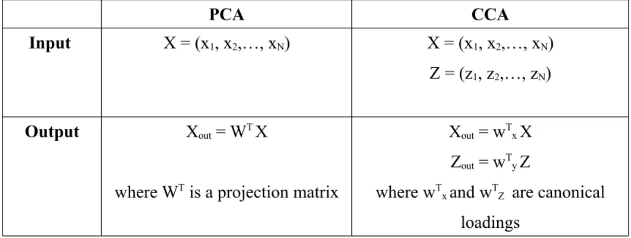
principal components, and to display the pattern of similarity of the observations. Table 1 compares the input and output of PCA and CCA

PCA CCA

Input X = (x1, x2,…, xN) X = (x1, x2,…, xN) Z = (z1, z2,…, zN)

Output Xout = WT X

where WT _{is a projection matrix}

Xout = wTxX Zout = wTyZ where wT

x and wTZ are canonical loadings

Table 1 A comparison between PCA and CCA

2.2.2 Pearson’s correlation coefficient

Pearson's correlation coefficient (r-value) is a measure of the strength of the associationbetween the two continuous variables. The r-value for continuous data ranges from -1 to +1. When r = -1, a perfect negative linear correlation is indicated. When r = 1, a perfect positive linear correlation is indicated. When r = 0, there is no relationship between the variables.

(17)

The formula for Pearson's correlation coefficient is:

ρ_{X , Z}=cov_σ(X , Z)

XσZ

Where X and Z are data vectors. ‘cov’ is the covariance.

‘σX’ and ‘σZ’ are the standard deviations of X and Z respectively.

The interpretation of an r-value is comparable to the interpretation of a canonical correlation in that they both measure how strong two sets of data are correlated. The main difference is that the analysis of Pearson's correlation coefficient can take into account only one feature at a time for each set of data.

2.3 Probability distribution models for generating synthetic biological data

2.3.1 Multivariate Gaussian distribution

Multivariate Gaussian Distribution (or Multivariate Normal Distribution) is a generalization of the one-dimensional normal distribution to higher dimensions.

For a random-valued random variable x = [X1, X2, …., Xn]T

If μ is a n-dimensional mean vector and ∑ is the respective n×n covariance matrix

p(x ;μ,Σ)= 1 (2 π)n/2|_Σ|1/2exp(− 1 2(x−μ ) T Σ−1(x−μ ))

(18)

This can be written as

The gene-expression levels are modeled as a multivariate Gaussian distribution that statistically captures the real mRNA levels within the cells.

Σhas the following block structure:

Σ ρ is a square matrix, with 1 on the diagonal and ρ off the diagonal. All features in the same block are correlated to one another with the correlation coefficient ρ (which ranges from -1 to 1), while features of different blocks are uncorrelated.

2.3.2 Poisson distribution

The National Institute for Biological Standards and Control [5] defines Next Generation Sequencing (NGS) as technologies that offer high-throughput, rapid and

(19)

accurate methods of determining the precise order of nucleotides within DNA/RNA molecules.

The specific application of NGS for RNA sequencing is called RNA-Seq, which is a high-throughput measurement of gene-expression levels of thousands of genes simultaneously as represented by discrete expression values for regions of interest on the genome (e.g. genes).

According to Ghaffari et al. (2013) [6], two popular models for statistical representation of the discrete NGS data are the negative binomial and Poisson. The negative binomial model is more general because it can mitigate over-dispersion issues associated with the Poisson model; however, with the relatively small number of

samples available in most current NGS experiments, it is difficult to accurately estimate the dispersion parameter of the negative binomial model. Therefore, in this study, the RNA-seq model is a combination of a multivariate Gaussian (representing the genes' concentrations) followed by a Poisson process. This method overcomes the dispersion problems associated to the case where data is simply drawn from a Poisson distribution.

The expected number of reads (mean of the Poisson distribution) are calculated from the generalized linear model.

E[ Xi,j |si ] = si exp( λi,j + θi,j )

(20)

Xi,j is the read count for gene j for sample point i

λi,j is the jth gene-expression level in lane i

θi,j represents technical effects that might be associated with an experiment. we

assume that it follows a Gaussian distribution with zero mean and a variance set by the coefficient of variation (COV). That is,

2.4 Current state of the computational website

The testing version of the APIMOD computational website is able to host two types of biological data analysis service, a sequencing classification and a differential gene expression. For the sequencing classification, users would submit RNAseq datasets and the tool would determine a pair of genes that differentiate the two sample

populations in the dataset. For the differential gene expression, the analysis is done for RNAseq data where the quantitative-biology-core computational pipeline is used to determine differential expression genes. Specifically, mapped reads are normalized and then the result together with the experiment key file are fed to a statistical package called EdgeR to determine differentially expressed genes.

To use the computation site, the users start by navigating on the website and selecting the analysis service of their choice. Figure 1 is the screen-shot of the interface

(21)

for users to choose between the two choices of analysis. Then they fill in a form describing their information, including name, e-mail, project name, and project descriptions. An example of the form is shown in Figure 2. Depending on the type of service chosen, different types of files are needed to be uploaded. A read file is required for the sequencing classification, and a key file and a count file are required for the differential expression. After filling out those required fields and submitting the service request, a confirmation email is sent to the users. The confirmation email would include a link that redirect the users to a status page, where their service detail as well as the current status are displayed. Once the status is ‘complete’, users are able to view the analysis results on the website as well as download them.

The internal structure of the website is constructed using Python (with Flask framework) and SQLite database. When a service request is submitted, a random identification number is generated and sent to the user, while the user’s information is stored in the computer that hosts the computational website. An SQLite database is used to keep track of the jobs submitted from the users. There are two groups in the database. One is for the analyses that are already completed and the other one is for the analyses waiting to be processed. Once each incomplete task is processed, it is transferred to the completed group.

(22)

Figure 1 The interface when users navigate the website. Users can click either on ‘Sequencing Classification’ or ‘Differential Expression’ to proceed to the next step.

(23)

3. RESEARCH DESCRIPTION

3.1 Problem definition

In recent years, an increasing amount of data has become more available in various fields, causing an upward trend in using statistical analysis to solve complicated problems. Researchers in the biology-related fields are among those that can utilize the great quantity of data. Research related to complex system requires a collection of various data types and the subsequent integrative analysis. Despite the meaningful insights statistical tools are able to provide, biologists often lack the adequate background in statistical computation and hesitate to use them.

The Chapkin Lab from the Nutrition department at Texas A&M University is one of the groups that use statistical tools in their research, which eventually leads to the motivation to host the APIMOD computational website. Other than the sequencing classification and differential expression, which are currently available for them, sparse CCA will also need to be added to the website.

Sparse CCA has been growing in popularity as a method for analyzing genomic data, where the number of features is far greater than the number of observations. To complete the whole process of canonical correlation analysis, multiple

data-preprocessing steps are required and some parameters have to be determined. People with expertise in statistical analysis might be able to perform those necessary steps until

(24)

the final results are achieved, but researchers with limited experience such as biologists, these steps might be too complicated. This is why it is highly significant to have an end-to-end computational tool that serves as a helper and makes sparse CCA approachable for all types of researchers.

3.2 Research goals

There are four main goals for the implementation of this sparse CCA computational tool.

1. Tool’s validation

The tool must be able to detect the linear relationship manually implemented in the synthetic data and to replicate results for real data

2. User-friendly implementation

The tool should be implemented in a very user-friendly way. Users should be guided to use the tool to achieve their research objectives without any need to consult an expert. 3. Code modularity

Sufficient code modularity should allow any adjustments or incoming data analysis methods to be implemented without complication.

(25)

4. Well-written documentation

Tool specification that allow for its seamless integration with the current APIMOD site must be provided.

(26)

4. PROJECT APPROACH

The sparse CCA computational tool is implemented in R and Python. To accomplish the research goal, the process as a whole is divided into several steps. 4.1 Frameworkdesign

The web-interface portion is implemented using a combination of both Python (Flask) and SQLite, a software library that implements a self-contained, server-less SQL database engine. Initially, users have to submit two files to the system as inputs, each as a CSV or TXT file containing a data table. The two tables must have the same number of samples (rows) but can have different number of features (columns). After submission, the inputs are saved into a specific folder set up in back-end system. Those inputs are then called when the computational code is executed. After the whole process is complete, the results are stored in another folder.

Ideally, the web-based tool will be able to accept many jobs and keep a record of the order of their submission to the system. A database will be set up for that purpose. Once each job is submitted by a user, the database will record its status as ‘incomplete’. Then the R code will process the incomplete job, and once the computational process is done, the database status will be changed to ‘complete’.

Each input’s expected format is a table with the same numbers of samples (rows). The preprocessing step will confirm that the format is acceptable before proceeding to the

(27)

next step. Also, due to the computational requirement of the sparse CCA, any columns of data with standard deviation equal to zero must be removed.

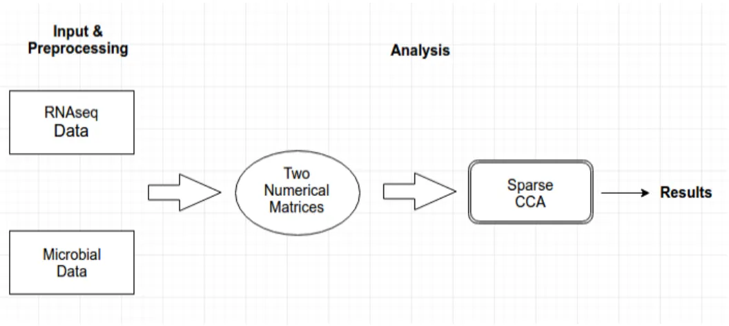
After preprocessing, the two input tables are now in the form of numerical matrices and ready to be analyzed. Those matrices will be used as input parameters for the sparse CCA functions from the R package ‘PMA’.The generated results are a score table and four graphs showing the component scores of the two inputs. The R package ‘ggplot2’[7] is used for generating the plots. Figure 3 is the diagram showing the tool’s workflow.

(28)

4.2 Implementing a sparse CCA method

‘PMA’ is an R package that performs penalized multivariate analysis. It offers a wide range of tools including the sparse CCA. The two functions related to the analysis that will be used are ‘CCA’ and ‘CCA.permute’. Below are the detailed descriptions referenced from the official manual of the package ‘PMA’ [8] on how these two functions can be used.

4.2.1 ‘CCA.permute’ function

‘CCA.permute’ automatically selects tuning parameters for sparse CCA using the penalized matrix decomposition, as described in Witten et al. (2009) [9]. For each data set X and Z, two types are possible: (1) type ‘standard’, which does not assume any ordering of the columns of the data set, and (2) type ‘ordered’, which assumes that columns of the data set are ordered and thus that corresponding canonical vector should be both sparse and smooth (e.g. CGH data). For X and Z, the samples are on the rows and the features are on the columns. The tuning parameters are selected using a permutation scheme. For each candidate tuning parameter value, the following is performed:

1. The samples in X are randomly permuted nperms times, to obtain matrices X*1,X*2,. …

(29)

2. Sparse CCA is run on each permuted data set (X*i , Z) to obtain factors (u*i , v*i), which are the canonical coefficients for each pair of (X*i , Z).

3. Sparse CCA is run on the original data (X, Z) to obtain factors u and v, which are the resulting canonical coefficients of X and Z respectively..

4. Compute c*i = cor(X*i u*i , Z v*i) and c = cor(Xu , Zv). Note: cor(x,y) refers to the correlation of x and y.

5. Use Fisher’s transformation to convert these correlations into random variables that are approximately normally distributed. Let Fisher(c) denote the Fisher transformation of c.

6. Compute a z-statistic for Fisher(c), using

Fisher(c)−mean(Fisher(c* )) sd(Fisher(c*))

The larger the z-statistic, the ‘better’ the corresponding tuning parameter value.

As a result, the x penalty and z penalty which result in the highest z-statistic are chosen to be used as part of the input arguments of the ‘CCA’ function.

Usage:

CCA.permute(x,z,typex=c("standard", "ordered"),typez=c("standard","ordered"), penaltyxs=NULL, penaltyzs=NULL, niter=3,v=NULL,trace=TRUE,nperms=25,

(30)

standardize=TRUE, chromx=NULL, chromz=NULL,upos=FALSE, uneg=FALSE, vpos=FALSE, vneg=FALSE,outcome=NULL, y=NULL, cens=NULL)

4.2.2 ‘CCA’ function

The function ‘CCA’ performs sparse canonical correlation analysis using the penalized matrix decomposition. The main parameters to be taken in are the data matrices and their matrix penalty details.

Given matrices X and Z, which represent two sets of features on the same set of samples, the function finds sparse u and v such that uT_XT_{Zv is large. For X and Z, the} samples are on the rows and the features are on the columns. X and Z must have same number of rows, but may (and usually will) have different numbers of columns. The columns of X and/or Z can be unordered or ordered. If unordered, then a lasso penalty will be used to obtain the corresponding canonical vector. If ordered, then a fused lasso penalty will be used; this will result in smoothness.

Usage:

CCA(x, z, typex=c("standard", "ordered"),typez=c("standard","ordered"), penaltyx=NULL, penaltyz=NULL, K=1, niter=15, v=NULL, trace=TRUE,

standardize=TRUE, xnames=NULL, znames=NULL, chromx=NULL, chromz=NULL, upos=FALSE, uneg=FALSE, vpos=FALSE, vneg=FALSE, outcome=NULL, y=NULL, cens=NULL)

(31)

4.3 Performance evaluation

To test efficiency of the tool, multiple data sets are used in various scenarios. We first tested the sparse CCA tool on synthetic data sets generated according to the

algorithms and their implementations in Ghaffari et al. (2013) [6], Yousefi et al. (2011) [10], and Bahadorinejad, A. (2017) [11]. Once being successful with the synthetic datasets, real datasets are next considered.

For synthetic datasets, there are three types of data being generated, which are the multivariate Gaussian Data, the RNAseq data, and the microbial sequencing data. The multivariate Gaussian data model is based on the multivariate Gaussian distribution. The model has a blocked covariance structure that conforms to various observations made in microarrray expression-based studies [10]. For the RNAseq data, the model used is a combination between the general model based on multivariate Gaussian distribution followed by a transformation based on Poisson distribution model. A series of distribution models can be constructed by changing model parameters to generate different synthetic data samples. For the microbial sequencing data, a python script is used to simulate Operational Taxonomic Units (OTU) frequency vectors that take into account phylogenetic relatedness of OTUs.

We also tested the sparse CCA tool on a real data set generated during the NIH-funded project “Gut Mibrobiota And Colonic Gene Expression: A Lingan Trial In Humans”, co-conducted by the Nutrition Department at Texas A&M University.

(32)

4.3.1 Applying sparse CCA to synthetic data

There are three sets of data being randomly generated: microbial sequencing, multivariate Gaussian, and RNA sequencing. The RNA sequencing data is generated by processing the multivariate Gaussian data through a Poisson process.

First, two canonical correlations are computed, one is between the microbial sequencing and the multivariate Gaussian data and the other one is between the microbial sequencing and RNA sequencing data. Then, we implement a linear

relationship between each pair of data. After the linear relationships are constructed, the two canonical correlations are computed again on the same variables, then the two sets of values are compared.

4.3.1.1 Methods for generating synthetic data

There are three types of synthetic data generated: Microbial OTUs, Multivariate Gaussian, and RNA sequencing (RNAseq).

The code for generating microbial sequencing data is written in Python by Arghavan Bahadorinejad [11]. It basically simulates OTU frequency vectors that take into account phylogenetic relatedness of OTUs.

For generating multivariate Gaussian data, the code was written in C++ by Jianping Hua, as described in Yousefi et al. (2011) [10]. The simulation design uses a general model based on multivariate Gaussian distributions with a blocked covariance structure that conforms to various observations made in microarray expression-based

(33)

studies. A battery of distribution models can be constructed by changing model

parameters to generate different synthetic data samples. The Gaussian distribution model simulates RNA concentrations in real samples.

RNAseq data is generated by the code that was an extension of the one that generates the multivariate Gaussian data, as described in Ghaffari et al. (2013) [6]. After the multivariate Gaussian data is generated, it is pushed through a Poisson process. The Poisson transformation simulates using the sequencing machine in the real experiment. Figure 4 is the flow diagram for generating both the Multivariate Gaussian and RNAseq data.

(34)

4.3.1.2 Linear relationship implementation

Since sparse CCA is an analysis that detects linear relationships between two sets of data and the synthetic data are randomly generated, it is necessary that relationships are manually implemented so that the sparse CCA can be tested. The built-in R function ‘lm’ is used to fit the randomly generated data. The fitted data will be in the form

∑ yk = ∑ aixi + intercept

where ‘k’ and ‘i’ are the indexes related to OTUs and genes used to be included in the linear implementation respectively. Different ranges of ‘k’ and ‘i’ are used so that the results in different scenarios can be compared against one another. Only genes from multivariate Gaussian are used in the implementation in order to observe how the Poisson process affects the linear relationships.

4.3.2 Applying sparse CCA to real data

To further validate the sparse CCA tool, we attempt to replicate the unpublished study “An application of sCCA for integrative analysis of diet-dependent interaction between gut microbiota and host in neonates” [12]. Additional results not included in the original study are also supplied in order to strengthen the validation. The study applies sparse CCA on a pair of host microarray data set and microbial data set, which was aligned using Rapid Annotation using Subsystems Technology (MG-RASTv2) against the SEED subsystem database.

(35)

The input for the tool’s validation is already in the acceptable form of two tables, resulting from the preprocessing step that was done separately. Quantile normalization was used for RNAseq data while an R package ‘metagenomeSeq’ [13] was used for the microbial sequencing data. It is possible to add these normalization methods to the tool in the future using steps similar to the explanation made in APPENDIX C.

(36)

5. RESULTS

5.1 Tool framework

The sparse CCA computational tool is implemented using the structure similar to that of the sequencing classification and differential expression analysis, so that they can be easily integrated on the website. Specifically, the same tools and folders organization are utilized when building the sparse CCA application. An important feature introduced in the implementation is the modularity of the tool, which allow ease of addition of any new tools in the future. The code component comprised of two major parts. The first part is the one that handles all relations between a user’s input, database, and the analysis portion. The other part is the data analysis part.

For the first part, the code initially checks if there is any file in the database. If there is no file, then the process stops. If a file exists, the database is connected using an R package “RSQLite” [14]. Then the database checks for a job with an ‘incomplete’ status, which will eventually be processed. If none of the jobs has the status of ‘incomplete’, the process also ends.

The second part of the code component handles the computational portion. Particularly, it is the part where the sparse CCA is implemented. The code is placed within the error handling function called tryCatch, which is inside the first part. This way of implementation allows the modularity feature to be possible. That is the code

(37)

inside the tryCatch function can be replaced with other types of computational methods in order to add more functionality to the tool.

5.2 Synthetic data

After the sparse CCA is implemented, it is then applied to multiple datasets. Many scenarios for each dataset are considered.

5.2.1 Small number of features

The key property to be considered is the canonical cross loadings, which is the correlation of each variable with the opposite canonical variate.

The data consists of 2 OTUs and 3 genes. We use U1 as the canonical variate for the microbial data, V1 as the canonical variate for the multivariate Gaussian data, and W1 as the canonical variate for the RNAseq data. Table 2 through Table 13 show the canonical cross loadings for each variable in each dataset both before and after the linear relationship is implemented.

In the linear implementation, microbial data is used as a dependent variable while the multivariate Gaussian or RNA sequencing data is used as independent variables. There are three cases in this numerical experiment. Each case has the form of y1 ~ ∑ xk where ‘k’ ranges from 1 to 3. The notation ‘~’ indicates a linear relationship. For

(38)

example, y ~ x1+x2 is equivalent to the form y = m1x1+m2x2+ c where m1 and m2 are slopes and c is a constant.

(39)

Case 1: OTU1 ~ Gene1

Table 2 Canonical cross-loadings between the canonical variate for the multivariate Gaussian data and each of the OTUs, with OTU1 and Gene1 being used in the linear implementation V1 vs. OTUs OTU 1 OTU 2 Dataset 1 Before -0.3907183 -0.1186813 After -1 -0.2260459 Dataset 2 Before -0.1391491 0.0585454 After -1 0.06826512 Dataset 3 Before -0.4217921 0.0407734 After -1 0.1365645 Dataset 4 Before -0.195657 -0.302892 After -1 -0.302892 Dataset 5 Before -0.4110796 -0.3802128 After -1 -0.1696654 Dataset 6 Before 0.0009457134 0.36187219 After -1 -0.1616121 Dataset 7 Before -0.0350365 -0.3819603 After -1 0.0793762 Dataset 8 Before -0.2686624 -0.0550798 After -1 -0.2188731 Dataset 9 Before -0.074364 0.369191 After -1 -0.0083163 Dataset 10 Before -0.32068989 -0.06316337 After -1 -0.1439532 Dataset 11 Before -0.42211989 -0.0194381 After -1 0.0958877

(40)

Table 3 Canonical cross-loadings between the canonical variate for the microbial data and each of the genes in the multivariate Gaussian data, with OTU1 and Gene1 being used in the linear implementation

U1 vs. Genes

Gene 1 Gene 2 Gene 3

Dataset 1 Before 0.01870357 0.35116653 0.14620568 After 1 0.2294226 -0.2968851 Dataset 2 Before 0.06022922 -0.12502358 -0.03120631 After 1 0.1613756 -0.1149653 Dataset 3 Before -0.3498769 -0.2936249 0.1429806 After -1 -0.0481509 0.0795961 Dataset 4 Before -0.3028919 -0.0242343 -0.2212093 After -1 -0.1386472 -0.1513016 Dataset 5 Before 0.3590944 -0.2340555 -0.362238 After 1 -0.208301 -0.1264478 Dataset 6 Before 0.1616121 -0.3113451 0.1293518 After -1 -0.30304246 0.04346897 Dataset 7 Before -0.0793762 -0.3666335 0.1342536 After 1 0.3011729 0.0042999 Dataset 8 Before -0.0912606 0.1299878 0.2418749 After -1 -0.3104978 -0.1376715 Dataset 9 Before 0.008316298 0.312365 -0.20366 After -1 -0.0589381 0.0059786 Dataset 10 Before -0.1364311 -0.2840887 0.1965004 After -1 -0.1550587 0.1237826 Dataset 11 Before -0.040835 0.4221199 -0.0133788 After -1 0.2846204 0.3264974

(41)

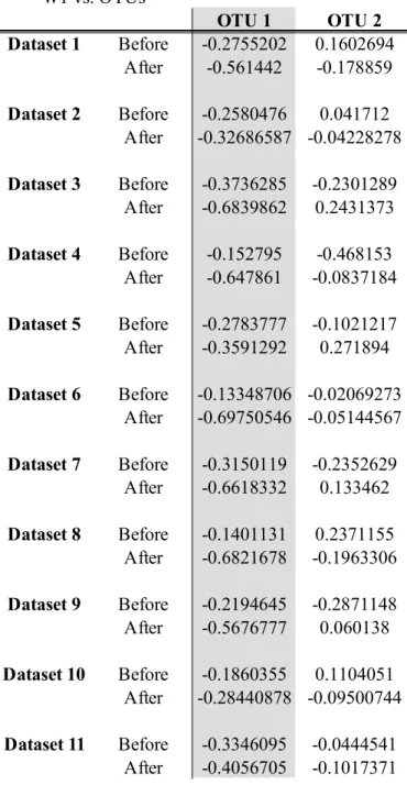
Table 4 Canonical cross-loadings between the canonical variate for the RNAseq data and each of the OTUs, with OTU1 and Gene1 being used in the linear

implementation W1 vs. OTUs OTU 1 OTU 2 Dataset 1 Before -0.2755202 0.1602694 After -0.561442 -0.178859 Dataset 2 Before -0.2580476 0.041712 After -0.32686587 -0.04228278 Dataset 3 Before -0.3736285 -0.2301289 After -0.6839862 0.2431373 Dataset 4 Before -0.152795 -0.468153 After -0.647861 -0.0837184 Dataset 5 Before -0.2783777 -0.1021217 After -0.3591292 0.271894 Dataset 6 Before -0.13348706 -0.02069273 After -0.69750546 -0.05144567 Dataset 7 Before -0.3150119 -0.2352629 After -0.6618332 0.133462 Dataset 8 Before -0.1401131 0.2371155 After -0.6821678 -0.1963306 Dataset 9 Before -0.2194645 -0.2871148 After -0.5676777 0.060138 Dataset 10 Before -0.1860355 0.1104051 After -0.28440878 -0.09500744 Dataset 11 Before -0.3346095 -0.0444541 After -0.4056705 -0.1017371

(42)

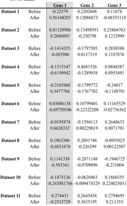
Table 5 Canonical cross-loadings between the canonical variate for the microbial data and each of the genes in the RNAseq data, with OTU1 and Gene1 being used in the linear implementation

U1 vs. Genes

Gene 1 Gene 2 Gene 3

Dataset 1 Before -0.22579 0.2202608 0.11878 After 0.56144203 0.12086873 -0.08553118 Dataset 2 Before 0.01129986 -0.13498591 0.25804763 After 0.2696895 -0.250798 0.1232999 Dataset 3 Before -0.1414355 -0.1797505 0.2830388 After -0.683986 0.0137319 0.1107876 Dataset 4 Before -0.1315147 0.4681526 0.0846587 After -0.6150942 -0.1289938 0.0955491 Dataset 5 Before -0.2103968 -0.1799772 -0.24017 After 0.3477704 -0.1767702 -0.1149791 Dataset 6 Before 0.03006138 0.10799401 0.11165529 After -0.69750546 -0.22322208 -0.02736362 Dataset 7 Before -0.0195874 -0.1594113 0.2648633 After 0.6628332 0.00229019 0.0071701 Dataset 8 Before 0.1963306 0.2091746 -0.0955025 After -0.6821678 -0.226299 0.00122507 Dataset 9 Before 0.1141338 -0.2871148 -0.1946725 After -0.503361 -0.0709896 -0.231004 Dataset 10 Before -0.1475136 -0.0626963 0.1860355 After -0.243881766 -0.009474329 0.224025031 Dataset 11 Before 0.274431 0.2645438 0.2794695 After -0.2513729 0.3635195 0.211355

(43)

Case 2: OTU1 ~ Gene1 + Gene2

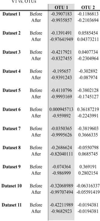
Table 6 Canonical cross-loadings between the canonical variate for the multivariate Gaussian data and each of the OTUs, with OTU1, Gene1, and Gene2 being used in the linear implementation

V1 vs. OTUs OTU 1 OTU 2 Dataset 1 Before -0.3907183 -0.1186813 After -0.9935857 -0.2103694 Dataset 2 Before -0.1391491 0.0585454 After -0.97641949 0.04373211 Dataset 3 Before -0.4217921 0.0407734 After -0.8327455 -0.2304964 Dataset 4 Before -0.195657 -0.302892 After -0.9391243 -0.087974 Dataset 5 Before -0.4110796 -0.3802128 After -0.9993169 -0.1745127 Dataset 6 Before 0.000945713 0.36187219 After -0.959892 -0.2243991 Dataset 7 Before -0.0350365 -0.3819603 After -0.9995626 0.3666335 Dataset 8 Before -0.2686624 -0.0550798 After -0.82040111 0.0685745 Dataset 9 Before -0.074364 0.369191 After -0.986999 0.2802154 Dataset 10 Before -0.32068989 -0.06316337 After -0.99707494 -0.05591419 Dataset 11 Before -0.42211989 -0.0194381 After -0.9682923 -0.0194381

(44)

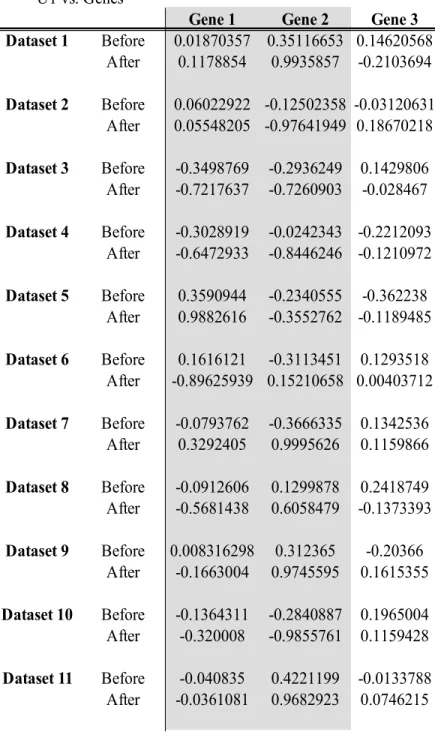
Table 7 Canonical cross-loadings between the canonical variate for the microbial data and each of the genes in the multivariate Gaussian data, with OTU1, Gene1, and Gene2 being used in the linear implementation

U1 vs. Genes

Gene 1 Gene 2 Gene 3 Dataset 1 Before 0.01870357 0.35116653 0.14620568 After 0.1178854 0.9935857 -0.2103694 Dataset 2 Before 0.06022922 -0.12502358 -0.03120631 After 0.05548205 -0.97641949 0.18670218 Dataset 3 Before -0.3498769 -0.2936249 0.1429806 After -0.7217637 -0.7260903 -0.028467 Dataset 4 Before -0.3028919 -0.0242343 -0.2212093 After -0.6472933 -0.8446246 -0.1210972 Dataset 5 Before 0.3590944 -0.2340555 -0.362238 After 0.9882616 -0.3552762 -0.1189485 Dataset 6 Before 0.1616121 -0.3113451 0.1293518 After -0.89625939 0.15210658 0.00403712 Dataset 7 Before -0.0793762 -0.3666335 0.1342536 After 0.3292405 0.9995626 0.1159866 Dataset 8 Before -0.0912606 0.1299878 0.2418749 After -0.5681438 0.6058479 -0.1373393 Dataset 9 Before 0.008316298 0.312365 -0.20366 After -0.1663004 0.9745595 0.1615355 Dataset 10 Before -0.1364311 -0.2840887 0.1965004 After -0.320008 -0.9855761 0.1159428 Dataset 11 Before -0.040835 0.4221199 -0.0133788 After -0.0361081 0.9682923 0.0746215

(45)

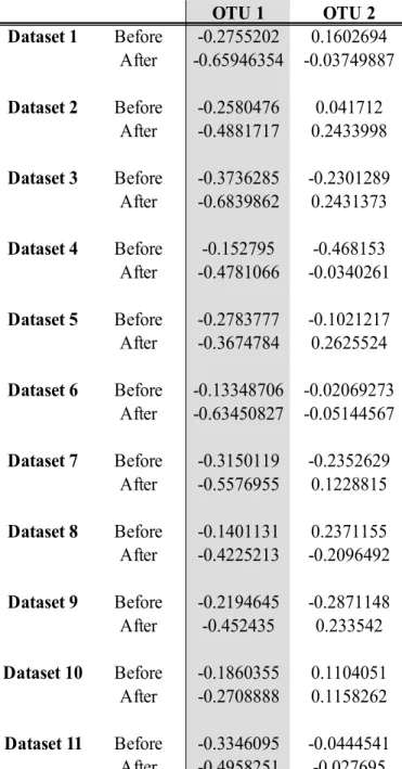
Table 8 Canonical cross-loadings between the canonical variate for the RNAseq data and each of the OTUs, with OTU1, Gene1 and Gene2 being used in the linear implementation W1 vs. OTUs OTU 1 OTU 2 Dataset 1 Before -0.2755202 0.1602694 After -0.65946354 -0.03749887 Dataset 2 Before -0.2580476 0.041712 After -0.4881717 0.2433998 Dataset 3 Before -0.3736285 -0.2301289 After -0.6839862 0.2431373 Dataset 4 Before -0.152795 -0.468153 After -0.4781066 -0.0340261 Dataset 5 Before -0.2783777 -0.1021217 After -0.3674784 0.2625524 Dataset 6 Before -0.13348706 -0.02069273 After -0.63450827 -0.05144567 Dataset 7 Before -0.3150119 -0.2352629 After -0.5576955 0.1228815 Dataset 8 Before -0.1401131 0.2371155 After -0.4225213 -0.2096492 Dataset 9 Before -0.2194645 -0.2871148 After -0.452435 0.233542 Dataset 10 Before -0.1860355 0.1104051 After -0.2708888 0.1158262 Dataset 11 Before -0.3346095 -0.0444541 After -0.4958251 -0.027695

(46)

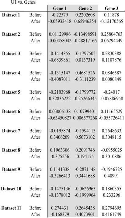
Table 9 Canonical cross-loadings between the canonical variate for the microbial data and each of the genes in the RNAseq data, with OTU1, Gene1 and Gene2 being used in the linear implementation

U1 vs. Genes

Gene 1 Gene 2 Gene 3 Dataset 1 Before -0.22579 0.2202608 0.11878 After -0.05933418 0.65946354 -0.12170565 Dataset 2 Before 0.01129986 -0.13498591 0.25804763 After -0.00458042 -0.48817166 0.06294449 Dataset 3 Before -0.1414355 -0.1797505 0.2830388 After -0.6839861 0.0137319 0.1107876 Dataset 4 Before -0.1315147 0.4681526 0.0846587 After -0.4087011 -0.3111239 0.0080849 Dataset 5 Before -0.2103968 -0.1799772 -0.24017 After 0.32836222 -0.25266345 -0.07886958 Dataset 6 Before 0.03006138 0.10799401 0.11165529 After -0.63450827 0.006577268 -0.055726411 Dataset 7 Before -0.0195874 -0.1594113 0.2648633 After 0.3406209 0.5073102 0.3048115 Dataset 8 Before 0.1963306 0.2091746 -0.0955025 After -0.375256 0.194175 0.3010886 Dataset 9 Before 0.1141338 -0.2871148 -0.1946725 After -0.3266413 0.3441688 0.40991 Dataset 10 Before -0.1475136 -0.0626963 0.1860355 After -0.1378012 -0.1999964 0.233296 Dataset 11 Before 0.274431 0.2645438 0.2794695 After -0.168379 0.4073901 0.4161749

(47)

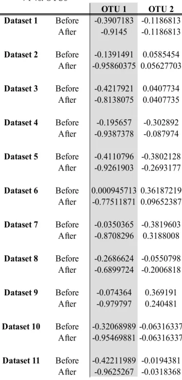
Case 3: OTU1 ~ Gene1 + Gene2 + Gene3

Table 10 Canonical cross-loadings between the canonical variate for the multivariate Gaussian data and each of the OTUs, with OTU1, Gene1, Gene2, and Gene3 being used in the linear implementation

V1 vs. OTUs OTU 1 OTU 2 Dataset 1 Before -0.3907183 -0.1186813 After -0.9145 -0.1186813 Dataset 2 Before -0.1391491 0.0585454 After -0.95860375 0.05627703 Dataset 3 Before -0.4217921 0.0407734 After -0.8138075 0.0407735 Dataset 4 Before -0.195657 -0.302892 After -0.9387378 -0.087974 Dataset 5 Before -0.4110796 -0.3802128 After -0.9261903 -0.2693177 Dataset 6 Before 0.000945713 0.36187219 After -0.77511871 0.09652387 Dataset 7 Before -0.0350365 -0.3819603 After -0.8708296 0.3188008 Dataset 8 Before -0.2686624 -0.0550798 After -0.6899724 -0.2006818 Dataset 9 Before -0.074364 0.369191 After -0.979797 0.240481 Dataset 10 Before -0.32068989 -0.06316337 After -0.95469881 -0.06316337 Dataset 11 Before -0.42211989 -0.0194381 After -0.9625267 -0.0318368

(48)

Table 11 Canonical cross-loadings between the canonical variate for the microbial data and each of the genes in the multivariate Gaussian data, with OTU1, Gene1, Gene2, and Gene3 being used in the linear implementation

U1 vs. Genes

Gene 1 Gene 2 Gene 3 Dataset 1 Before 0.01870357 0.35116653 0.14620568 After 0.0294174 0.8181304 0.3616538 Dataset 2 Before 0.06022922 -0.12502358 -0.03120631 After 0.01572789 -0.88187657 0.60357339 Dataset 3 Before -0.3498769 -0.2936249 0.1429806 After -0.6575814 -0.615524 0.4498756 Dataset 4 Before -0.3028919 -0.0242343 -0.2212093 After -0.6473556 -0.8442025 -0.0972547 Dataset 5 Before 0.3590944 -0.2340555 -0.362238 After 0.7781259 -0.3269968 -0.6914781 Dataset 6 Before 0.1616121 -0.3113451 0.1293518 After -0.6650068 0.1141568 0.6699263 Dataset 7 Before -0.0793762 -0.3666335 0.1342536 After 0.3398491 0.7469429 0.7325247 Dataset 8 Before -0.0912606 0.1299878 0.2418749 After -0.551744 0.5320788 0.2509534 Dataset 9 Before 0.0083163 0.312365 -0.20366 After -0.142493 0.9383129 0.4348558 Dataset 10 Before -0.1364311 -0.2840887 0.1965004 After -0.2900495 -0.834644 0.6207757 Dataset 11 Before -0.040835 0.4221199 -0.0133788 After -0.021954 0.953491 -0.0742191

(49)

Table 12 Canonical cross-loadings between the canonical variate for the RNAseq data and each of the OTUs, with OTU1, Gene1,Gene2, and Gene3 being used in the linear implementation W1 vs. OTUs OTU 1 OTU 2 Dataset 1 Before -0.2755202 0.1602694 After -0.53361876 0.001315121 Dataset 2 Before -0.2580476 0.041712 After -0.4736886 0.2433998 Dataset 3 Before -0.3736285 -0.2301289 After -0.5196779 0.2040253 Dataset 4 Before -0.152795 -0.468153 After -0.4740843 -0.0340261 Dataset 5 Before -0.2783777 -0.1021217 After -0.37496202 -0.03444462 Dataset 6 Before -0.13348706 -0.02069273 After -0.52145469 -0.04873572 Dataset 7 Before -0.3150119 -0.2352629 After -0.5172044 0.153402 Dataset 8 Before -0.1401131 0.2371155 After -0.5053266 -0.097944 Dataset 9 Before -0.2194645 -0.2871148 After -0.5037548 0.2257296 Dataset 10 Before -0.1860355 0.1104051 After -0.5052626 0.1104051 Dataset 11 Before -0.3346095 -0.0444541 After -0.4759663 -0.1445503

(50)

Table 13 Canonical cross-loadings between the canonical variate for the microbial data and each of the genes in the RNAseq data, with OTU1, Gene1, Gene2, and Gene3 being used in the linear implementation

U1 vs. Genes

Gene 1 Gene 2 Gene 3 Dataset 1 Before -0.22579 0.2202608 0.11878 After -0.24565406 0.49620364 0.06590824 Dataset 2 Before 0.01129986 -0.13498591 0.25804763 After 0.06893597 -0.47368864 0.27986026 Dataset 3 Before -0.1414355 -0.1797505 0.2830388 After -0.4653387 -0.1154333 0.4155736 Dataset 4 Before -0.1315147 0.4681526 0.0846587 After 0.4037761 -0.3156223 0.0202176 Dataset 5 Before -0.2103968 -0.1799772 -0.24017 After 0.1566423 -0.2504334 -0.3273299 Dataset 6 Before 0.03006138 0.10799401 0.11165529 After -0.45793806 -0.08802108 0.28627804 Dataset 7 Before -0.0195874 -0.1594113 0.2648633 After 0.2949942 0.4179895 0.4339231 Dataset 8 Before 0.1963306 0.2091746 -0.0955025 After -0.2600955 0.2516163 0.4542582 Dataset 9 Before 0.1141338 -0.2871148 -0.1946725 After -0.3073681 0.3183115 0.4647377 Dataset 10 Before -0.1475136 -0.0626963 0.1860355 After -0.07878463 -0.064644 0.50526263 Dataset 11 Before 0.274431 0.2645438 0.2794695 After -0.1379086 0.4176939 0.3195154

(51)

5.2.2 Large number of features

For cases where the number of features greatly exceeds the number of samples (with ratio of approximately 10:1 in this experiment), only the canonical correlations are considered instead of the cross-loadings as in the case of small features. The graphs (Figure 5 to Figure 12) show the canonical correlations for each case, where the number of genes ranges from 1 to 10.

(52)

2 OTUs, 1-10 genes

The plots show the canonical correlations after the linear relationship implementation for both the multivariate Gaussian and RNAseq data. The y-axis represents the canonical correlations while the x-axis represents the number of genes used in the implementation. The canonical correlations before the linear relationship implementation are 0.6966727 and 0.7593742 for multivariate Gaussian and RNA sequencing respectively.

Figure 5 The canonical correlation of the Multivariate Gaussian data after the linear implementation using 2 OTUs

(53)

Figure 6 The canonical correlation of the RNAseq data after the linear implementation, using 2 OTUs

3 OTUs, 1-10 genes

(54)

(55)

4 OTUs, 1-10 genes

(56)

5 OTUs, 1-10 genes

(57)

(58)

5.3 Real data

The real data consists of a host microarray data set and a microbial data set. The objective of this unpublished study we try to replicate is to apply the sparse CCA on this pair of data sets. In that study, both of the input data were not in the right format (as described in APPENDIX A) for the sparse CCA tool, and thus required some manual preprocessing steps before applying sparse CCA. In our replication, however, we start with two data files that are already in the correct format so that they are suitable for the tool. For the following plots, ‘Immunology’ refers to the microarray data set and ‘SeedLevel2’ refers to the microbial dataset. The elliptic shapes in each plot group the similar samples together.

5.3.1 SeedLevel2 vs. Immunology

Both Figure 13 and Figure 14 display the component scores of ‘SeedLevel2’ versus the component scores of ‘Immunology’. Figure 13 represents the first component scores while Figure 14 represents the second component scores. The canonical

correlation for the first component scores is 0.964 and the canonical correlation for the second component scores is 0.938.

(59)

Figure 13 The first component score between Immunology and SeedLevel2

(60)

5.3.2 First component scores vs. second component scores

Figure 15 shows the first component scores versus the second component scores of ‘SeedLevel2’. In order to display more than two dimensions, the first component scores of ‘Immunology’ is also shown using the color spectrum. Different feeding types for each sample is also represented by the circular and triangular shapes. Similarly, Figure 16 shows the first component scores versus the second component scores of ‘Immunology’. The first component scores of ‘SeedLevel2’ is also shown via the color spectrum.

(61)

Figure 16 The first component scores vs. the second component scores of Immunology

5.3.3 Sparse PCA

To illustrate that sparse CCA can separate two feeding types better than sparse PCA, the sparse PCA plots are provided as a comparison. Figure 17 represents the PCA scores for ‘SeedLevel2’ while Figure 18 represents the PCA scores for ‘Immunology’. The x-axis represents the first principle component scores while the y-axis represents the second principle component scores. The plots are generated from the Sparse PCA code that are manually implemented using the R package ‘PMA’, which is the same package used in the sparse CCA tool’s back-end.

(62)

Figure 17 The first vs. second PCA scores of SeedLevel2

(63)

6. DISCUSSION

6.1 Synthetic data

6.1.1 Small numbers of features

In this particular part of our validation studies, the data consists of 2 OTUs and 3 genes as features. We consider three separate cases. To solidify the results, each case is repeated with 12 different datasets. The reason for using small numbers of features is that it would be easier to detect the implemented linear relationship. Given that the numbers of features are small, the canonical cross loadings for each feature can easily be tracked. Each case of the numerical experiments results in four tables that display canonical cross-loadings (two for multivariate Gaussian data and two for RNA sequencing data).

The linear relationship is introduced between the variables from the multivariate Gaussian and the OTUs because the multivariate Gaussian models gene RNA

concentrations before the library preparation and the subsequent sequencing of those libraries. The first case to consider is when one OTU and one gene are used to construct the linear relationship. Table 1 shows the canonical cross-loadings between each of the OTUs and the canonical variate of the multivariate Gaussian data. Similarly, Table 2 shows the canonical cross-loadings between each of the genes and the canonical variate of the microbial data. After the relationship is introduced, the canonical cross-loadings

(64)

for the features used in the implementation increase as expected. Table 3 shows the canonical cross-loadings between each of the OTUs and the canonical variate of RNA sequencing data. Table 4 shows the canonical cross-loadings between each of the genes and the canonical variate of the microbial data. Unlike the multivariate Gaussian, the canonical cross-loadings do not display stable results, meaning that the cross-loadings do not always increase. Although most of the numbers do increase, the level of increments are lower than that of the multivariate Gaussian data.

For the second and third cases, where two and three genes are used in the linear relationship implementation respectively, the correlation can also be detected by the sparse CCA tool. For the multivariate Gaussian data, the absolute values of canonical cross loadings increase greatly. With the RNAseq data, however, the linear relationship can still be traced but it is not as obvious as the multivariate Gaussian cases. These results agree with the first case mentioned earlier. Nonetheless, there is a subtle

difference when using more than one features in the linear relationship implementation. The canonical cross-loadings for all features do not always increase altogether since the weight of each feature on the linear relationship is not the same.

The results from all three cases indicate that the transformation of the

multivariate Gaussian by the Poisson negatively affects the ability of the sparse CCA to detect the linear relationships introduced between the multivariate Gaussian and the OTUs. This suggests that one should use caution when interpreting the sparse CCA results where only sequencing data is used.

(65)

6.1.2 Large numbers of features

The numerical experiment for large numbers of features are performed in five scenarios. 789 OTUs are used for microbial data and 300 genes are used for both multivariate Gaussian data and RNA-sequencing data. Similar to the small cases, the linear relationship is introduced between the variables from the multivariate Gaussian and the OTUs. Between two to five OTUs are selected to have a linear relationship with one to ten genes. The chosen OTUs are those that have the minimum number of zero count among the samples. The genes, on the other hand, can be randomly selected.

Each pair of plots display the canonical correlations after implementing the relationship. The five cases presented are based on the number of OTUs in the linear relationship implementation. There are two plots in each case, one for multivariate Gaussian and one for RNAseq. The vertical axis is the canonical correlation for each number of genes used in the implementation. Since the number of features is large, we consider a canonical correlation instead of the canonical cross-loading for each feature used in the previous section.

For 2 OTUs, the original values of the canonical correlation are 0.6966727 and 0.7593742 for multivariate Gaussian data and RNA-sequencing data respectively. In fact, these numbers are the same when different numbers of OTUs are used, since they are the numbers before introducing the linear relationship. Figure 5 shows that after the implementation of linear relationship, the canonical correlations between the microbial

(66)

data and multivariate Gaussian data significantly increase. For the RNAseq data, the difference is that after the linear relationship is implemented, the canonical correlations between the microbial data and RNAseq data do not increase as much as those for the multivariate Gaussian data, and some do not increase at all, as shown in Figure 6. Following the same trend of thought as in Ghaffari et al. (2013) [6], we speculated that the Poisson process, which is part of the RNAseq generating process, has contributed to the distortion of the linear relationship implemented at the level of the multivariate Gaussian and OTUs level. For the case where three, four , and five OTUs are used, the plots are comparable with those from two OTUs and thus solidify the results obtained in the cases of small number of features.

Similar to the conclusion for the small case, the sparse CCA results should be interpreted with caution in the case where only sequencing data is used because the results indicate that the transformation of the multivariate Gaussian by the Poisson negatively affects the ability of the sparse CCA to detect the linear relationships introduced between the multivariate Gaussian and the OTUs.

6.2 Real data

6.2.1 SeedLevel2 vs. Immunology

Figure 13 and 14 were not included in the original results of the study but are included here in order to aid the sparse CCA interpretation. They are the scatter plots of

(67)

the first and second canonical variate pair between the two datasets respectively. The canonical correlations between the datasets are also displayed at the top of each graph. The values of canonical correlation reflect how strong the two sets of features are correlated. Higher number indicates stronger correlation which results in a less scattered and more linear positioning of the samples on the graph. Thus, one way of interpretation is to see how much the graph fits to a linear line. The more it fits, the more correlation there is. For ‘SeedLevel2’ and ‘Immunology’, the canonical variate plots for both the first and second variate pairs have an obvious linear fit,indicating that the sparse CCA performs as expected since it could find the linear combinations of the original variables such that those linear combinations are strongly correlated.

6.2.2 First component scores vs. second component scores

Figure 15 and 16 are the plots of the first versus the second canonical variate. Figure 15 is for ‘SeedLevel2’ while Figure 16 is for ‘Immunology’. The tool is able to replicate the results made in the paper. For these two plots, the horizontal axis

corresponds to the first canonical variate and the vertical axis corresponds to the second canonical variate. In order to add a third dimension to the graph and see the relationship with another variable a color bar on the right is attached. When plotting the result this way, the samples could be separated into groups, based on their canonical variates. This suggest the potential use of the sparse CCA as not only a tool to detect correlations

(68)

between two sets of variables but also the ability to detect different phenotypes/classes presented by the samples.

6.2.3 Sparse PCA

The sparse PCA plots are used as a comparison in order to show the advantage of using sparse CCA. Spare PCA method was applied on both the host genes expression levels and gut microbiota data. For Figure 17, the x axis and y axis represent the first and second PCA components of the normalized second level of SEED subsystem

respectively. Similarly, for Figure 18, the x axis and y axis represent the first and second components of immunology related genes. It is noticeable that the sparse PCA method cannot separate the two groups of samples as well as the sparse CCA.

(69)

7. CONCLUSIONS

The sparse CCA tool is built based on the motivation that researchers without expertise in computational fields need to use statistical methods to solve their research related to integrative data analysis. A tool that is easy to use would allow them to

perform analyses without having to consult a statistical expert. The R package ‘PMA’ is the primary choice in the implementation because of its capability and efficiency in the sparse CCA computation. Moreover, this package also provides functions for computing a sparse PCA, so the future improvement of the tool will be relatively straightforward if such expansion is necessary.

The four significant objectives to be achieved are the tool’s validation, user-friendly implementation, code modularity, and a well-written documentation. For validation purposes, the sparse CCA tool is applied on synthetic datasets with manual implementation of linear relationship and is also applied on the real data to replicate the result from the unpublished study “An application of sCCA for integrative analysis of diet-dependent interaction between gut microbiota and host in neonates”. For synthetic data, both small and large numbers of features are used in order to confirm the validation results from synthetic data. For real data, supplementary plots that are not in the original study are also included to solidify the validation. The tool’s interface can guide users to complete their analyses, starting from the inputs preparation to the input submission. To

(70)

test the applicability of the tool, especially its user-interface portion, the tool was tried out by two of the lab members from the Chapkin lab. More details can be found in APPENDIX D. Internally, each part of the framework is designed to be modular so that additional tools can be implemented without complication. The documentation on the tool’s usage and specific methods on working with the framework are provided in APPENDIX A and APPENDIX C respectively.

The validation with synthetic data sets confirms the efficiency of the tool when being applied with multivariate Gaussian data. The validation experiments also show that one must be careful when applying the sparse CCA with RNAseq data because, unlike the multivariate Gaussian, the correlation cannot be easily detected due to the effect of the Poisson process transformation during the data generation. For the real data set, the tool is able to successfully replicate the results provided in the study, and thus prove its applicability to the real world problems.

The next step for the tool is to integrate it with the APIMOD website. The necessary steps are covered in the guideline provided in APPENDIX B. There are also a number of possible future extensions of the tool’s capability. One is to take advantage of the framework’s modularity feature and introduce more options to the tool such as normalization methods or another type of analysis such as the PCA. Another one is to validate more data types for sparse CCA. Although the tool currently is able to accept any type of data as inputs, as long as they have the same number of samples, there is no guarantee that the correlation will always be detected. Because multiple factors must be