Adaptive Robust Methodology for Parameter Estimation and Variable Selection

(1)

Clemson University

TigerPrints

All Dissertations

Dissertations

8-2017

Adaptive Robust Methodology for Parameter

Estimation and Variable Selection

Tao Yang

Clemson University, [email protected]

Follow this and additional works at:

https://tigerprints.clemson.edu/all_dissertations

This Dissertation is brought to you for free and open access by the Dissertations at TigerPrints. It has been accepted for inclusion in All Dissertations by an authorized administrator of TigerPrints. For more information, please [email protected].

Recommended Citation

Yang, Tao, "Adaptive Robust Methodology for Parameter Estimation and Variable Selection" (2017).All Dissertations. 2001.

(2)

Adaptive Robust Methodology for Parameter Estimation

and Variable Selection

A Dissertation Presented to the Graduate School of

Clemson University

In Partial Fulfillment of the Requirements for the Degree

Doctor of Philosophy Mathematical Sciences by Tao Yang August 2017 Accepted by:

Dr. Colin Gallagher, Committee Chair Dr. Christopher McMahan

Dr. Robert Lund Dr. Xiaoqian Sun

(3)

Abstract

The dissertation consists of three distinct but related projects. We consider regression model fitting, variable selection in regression, and autocorrelation estimation in time series. In each procedure we formulate the problem in terms of minimizing an objective function which adapts to the given data.

First we propose a robust M-estimation procedure for regression. The main purpose of the proposed methodology is to develop a procedure that adapts to light/heavy tailed, symmet-ric/asymmetric distributions with/without outliers. We focus on studying the properties of the maximum likelihood estimator of the asymmetric exponential power distribution, a broad distri-bution class that holds both Normal and asymmetric Laplace distridistri-butions as special cases. The proposed methodology unifies least squares and quantile regression in a data driven manner to cap-ture both tail decay and asymmetry of the underlying distributions. Finite sample performance of the method is exhibited via extensive Monte Carlo simulation and real data applications.

Second, we capitalize on the success of the proposed method and extend it to a variable selection procedure that selects the important predictors under a sparse setting. Quantile regression Lasso, i.e., quantile regession withL1norm on the regression coefficients for regularization is a robust technique to perform variable selection. However which quantile should be adopted is unclear. The proposed methodology introduces a way to choose the most “informative” quantile of interest that is used in the adaptive quantile regression Lasso. A modified BIC criterion is used to select the optimal tuning parameter. The proposed procedure selects the quantile based on the log-likelihood of the asymmetric Laplace distribution, and aims to perform the best quantile regression Lasso which is confirmed in both simulation study and a real data analysis.

Third, we focus on alleviating the underestimation issue of the sample autocorrelation in linear stationary time series. We first formulate autocorrelation estimation into a least squares

(4)

prob-lem and then apply a penalization to regulate the autocorrelation estimate. An adaptive sequence is proposed for tuning parameter and is shown to work well for stationary time series when the sample size is small and correlation is high.

(5)

Dedication

I dedicate this work to my loving parents, who always believe in me and support me in every step of the way.

(6)

Acknowledgments

First and foremost, I would like to show my deep gratitude to my advisors, Dr. Colin Gallagher and Dr. Christopher McMahan for their consistent support during the whole program. Especially, I want to thank Dr. Gallagher for his excellent mathematical insights that inspire me and thank Dr. McMahan for his extreme patience in the face of numerous obstacles. I could not have completed the work without their inspiration and advice.

I would also like to thank Dr. Robert Lund and Dr. Xiaoqian Sun for their serving on my committee, and thank to my fellow Ph.D. student Yan Liu for many discussions we had about details of research. In addition, I would like to thank the Department of Mathematics Sciences for providing financial support during my Ph.D. studies.

(7)

List of Tables

2.1 Simulation results summarizing the estimates of the ”slope” coefficient obtained by AME, LS, LAD, and ZQR, for both the AEPD and non-AEPD error distributions. This summary includes the average estimate minus the true value (Bias), relative efficiency (Eff), estimated coverage probability (Cov) associated with 95% confidence intervals, and averaged confidence interval length (AL). Here t3 denotes Student’s t-distribution with 3 degrees of freedom;χ2

3 denotes a Chi-square distribution with 3 degrees of freedom;SN(4) denotes a skewed normal distribution with a slant param-eter of 4;ST(3,0.5) for skewed t-distribution with 3 degrees of freedom and a skewing parameter of 0.5. . . 15 2.2 Blood pressure data analysis: Estimated regression coefficients, their estimated

stan-dard errors in parenthesis, and the values of the model selection criteria AIC and BIC, resulting from AME, LS, LAD, and ZQR. . . 19 3.1 Simulation results for coefficients estimates obtained by ALA, QR(τ) with τ ∈

{0.1,0.3,0.5,0.7,0.9} and PZQR for six distributions. This summary provides for the averaged estimate for each coefficient and the standard deviation of the estimates in parenthesis. . . 34 3.2 Variable selection results for six error distributions. This summary includes the

av-erage number of correctly specified zero coefficients (Correct), the avav-erage number of incorrectly specified zero coefficients (Wrong), and the averaged ˆτ. Here Norm Mix and Lap Mix denote the Normal mixture and Laplace mixture described in simulation section respectively. . . 36 3.3 Coefficients Estimates Result . . . 38 4.1 Simulation results summarizing the estimates of ρobtained by the sample

autocor-relation at lag one ˆρ and the proposed autocorrelation estimate at lag one ˜ρunder AR(1) and ARMA(1,1) model. This summary includes the average estimate minus the true value (bias), standard deviation (sd) and relative mean squared error (RMSE). 46 4.2 Simulation results summarizing the estimates of ρobtained by the sample

autocor-relation ˆρand the proposed methods ˜ρ, and the estimates of partial autocorrelation at lag two α by the sample partial autocorrelation ˆα and the proposed methods ˜α

under AR(2) model. This summary includes the average estimate minus the true value (bias), standard deviation (sd) and RMSE of ˆρwith respect to ˜ρ(R(ρ)), and

(9)

List of Figures

2.1 The AEPD densities for different parameter configurations. . . 9 2.2 Empirical power curves obtained under AME, LS, LAD, and ZQR. Heret3 denotes

Student’s t-distribution with 3 degrees of freedom;χ2

3 denotes a Chi-square distribu-tion with 3 degrees of freedom; SN(4) denotes a skewed normal distribution with a slant parameter of 4; ST(3,0.5) for skewed t-distribution with 3 degrees of freedom and a skewing parameter of 0.5. . . 17 2.3 QQ-plots and histogram of the residuals under AME, LS, LAD, and ZQR for the

blood pressure dataset. . . 20 3.1 Box plot of the MAE scores across six error structures for different methods. Here

Norm Mix and Lap Mix denote Normal mixture and Laplace mixture described in simulation section respectively. . . 37

(10)

Chapter 1

Introduction

Statistical inferences are usually based on assumptions and lots of statistical procedures rely on distributional models for the error term. Many assumed error structures, e.g. Normal distribu-tion closely describes the distribudistribu-tion of many practical data sets and is mathematical convenient to analyze the pattern in real applications, which many not be exactly true. We consider a robust methodology that allows data to choose the loss function, equivalently to choose underlying distribu-tions from a broad class of distribudistribu-tions for regression coefficients estimation and variable selection. Before introducing the idea of the proposed procedures, we first present a brief review on different robust methodologies.

Huber (1964)proposed M-estimation approach and later Huber (1973) extended this to a regression setting, walked toward a theory of robust estimation by introducing the following loss function: min β∈Rp+1 n X i=1 ρ(yi−x0iβ), (1.1) whereρ(·) is a non-constant function. Many regression methods can be viewed as an M-estimation procedure. E.g.,ρ(x) =x2 _{yields least squares (LS), an optimal procedure under Normal} distribu-tions but very sensitive to a slight amount of outliers in the data set. Quantile regression (QR) as an alternative robust method introduced byBassett and Koenker (1978)corresponds toρ(x) =ρτ(x), where the quantile loss function ρτ(x) = |x|{τ I(x≥ 0) + (1−τ)I(x < 0)}. To further improve on the efficiency of QR, Zou and Yuan (2008) developed a regression method called composite

(11)

quantile regression (CQR) which takes a sum of K quantile loss functions at preset quantiles; i.e.,

ρ(x) = PK

k=1ρτk(x), where τk = k/(1 +K), for k = 1,· · ·, K. Sun et al. (2013) further extend

the idea of CQR by assigning different weights to the quantiles used in the CQR loss function with

ρ(x) = PK

k=1wkρτk(x), This allows the weighted composite quantile regression (WCQR) to deal

with both symmetric and asymmetric error distributions, and the optimal weightswk’s are selected by minimizing the asymptotic variance of the estimator so that it allows the data to determine which quantiles should be weighted more or less. Another way to achieve robust is to adaptively choose the power which the residuals are raised to in the loss function. Agr`o (1992)proposedLp regression which is essentially by takingρ(x) =−lnf(x), wheref is the probability density function (pdf) of the generalized error distribution (GED) (see Subbotin, 1923), in which the shape parameterpand the regression coefficients are estimated simultaneously.

These motivate us to develop a procedure that actually chooses the loss function according to two critical information given by the data, the tail decay and the skewness of the underlying error structure. We seek a procedure that allows continuous transition of loss function from LS to QR depending on these two characteristics of the underlying distribution. In particular, we propose an M-estimation procedure with ρ(x) = −lnf(x), where f is the pdf of a general distribution called asymmetric exponential power distribution (AEPD) which holds many distributions, e.g., Normal, Laplace, asymmetric Laplace as special cases. The proposed method which is essentially the maximum likelihood estimation for mis-specified models estimates regression coefficients and two additional parametersα(tail decay) andτ (asymmetry) simultaneously, where the estimates of

αand τ determine the loss function for estimating regression coefficients. The details of the work are shown in Chapter 2.

We then capitalize on the success of the proposed methodology and extend it to regression coefficients estimation and variable selection simultaneously in Chapter 3. Least absolute shrinkage and selection operator (Lasso) first introduced by Tibshirani (1996)is a useful approach to select important predictors under sparse setting and adaptive Lasso developed byZou (2006)used adaptive weights to penalize coefficients differently further improved the performance of variable selection. ThenWu and Liu (2009)developed penalized QR for variable selection, i.e., QR Lasso which replaces the LS loss in Lasso/Adaptive Lasso by the quantile check loss function to achieve robust property in variable selection. However the performance of QR Lasso procedure relies on the quantile of interest. The efficiency of QR Lasso can drop drastically for different quantiles and which quantile should be

(12)

used to achieve the best performance for a given data is what we focus on Chapter 3. Following the same vein of the proposed methodology in Chapter 2, we propose a loss function to be minus log-likelihood of the asymmetric Laplace distribution (ALD), a special case of AEPD for α = 1, plus an adaptive L1 norm penalization for regression coefficients estimation and variable selection simultaneously. The maximum likelihood estimator based on ALD studied by Bera et al. (2016) is essentially a penalized QR which selects the most “informative” quantile, and we further extend it to propose a penalized log-likelihood which aims to choose the most efficient QR Lasso with the quantile of interest dictated by data.

In the last chapter of this dissertation, we focus on the estimation of autocorrelation function in linear stationary time series. Evidence shows that the standard error of simple estimator such as ordinary least squares (OLS) tends to be underestimated, and thus it produces narrower confidence intervals due to ignoring the correlation within error terms (seeBence, 1995,Cochrane and Orcutt, 1949, anHurlbert, 1984). Bence (1995)considered adjustment which depends on accurate estimation of the autocorrelation at lag one (ρ). Sample autocorrelation which is widely used in time series is a consistent estimate of population autocorrelation and asymptotic normality was established. However it is quite generally realized that sample autocorrelation is liable to bias. The bias is usually negative which is common to many other estimation techniques, e.g., two-step Cochrane-Orcutt, the Durbin estimator, or maximum-likelihood estimation (see Park and Mitchell, 1980, Beesley and Griffiths, 1982,Griffiths and Beesley, 1984,King and Giles, 1984). And the bias issue deteriorates when sample size is smaller and absolute value ofρgets larger. In Chapter 4 we focus on applying a penalization idea to alleviate this issue. From a best linear predictor point of view, the problem can be formulated into a penalized LS, where the penalization is to adaptively “drag” theρestimate toward±1 so that underestimation issue can be alleviated.

(13)

Chapter 2

A robust regression methodology

via M-estimation

2.1

Introduction

Regression is the most common and useful statistical tool which can be used to quantify the relation-ship between a response variable (y) and explanatory variables (x). To this end, the seminal works of both Legendre in 1805 and Gauss in 1809 proposed the method of least squares (LS), which has arguably become the most popular approach to conducting a regression analysis. This popularity is likely attributable to the fact that the LS estimator can be expressed in closed form and can be shown to achieve minimum variance among all unbiased estimators, when the underlying error distribution is normal; e.g., see Rao (1945). However, this approach does not provide an optimal estimator for non-normal settings and is very sensitive to outlying observations (Koenker and Bas-sett, 1978). Further, experience has shown that LS regression may not be appropriate when the response variable differs from the regression function in an asymmetric manner, which is commonly encountered in medical data, among other venues. In lieu of these deficiencies, herein a general regression methodology is proposed which allows for the possibility of non-normal tail behavior and asymmetry in the conditional distribution of y given x, but will still perform well for symmetric and/or normally distributed data.

(14)

influence of outlying observations is to replace the LS loss function (i.e., the squared error loss) by a loss function which can accommodate asymmetry in the error distribution and is less susceptible to the magnitude of the residuals. For example, in 1793 Laplace proposed least absolute deviations (LAD), orL1-norm regression as an alternative to LS. This regression technique is less sensitive to outlying observations and is more appropriate, when compared to LS, for error distributions whose tails are heavier than that of the normal. More generally one can replace the LAD estimator, with an Lp norm estimator; for further discussion see Zeckhauser and Thompson (1970), Mineo (1989) and Agr`o (1992). Quantile regression estimates are found by minimizing the quantile (check) loss function, and since they estimate quantiles of the conditional distribution of y given x, they are appropriate for asymmetric and heavy tailed distributions (Koenker and Bassett, 1978).

Each of the aforementioned loss functions have corresponding conditional distributions of y givenxfor which the maximum likelihood estimator (MLE) is equivalent to the estimator which minimizes the corresponding loss: the LS estimator corresponds to the MLE when the error distri-bution is normal; the LAD estimator is equivalent to the MLE under Laplace errors, theLp norm estimator corresponds to the MLE when the error terms obey the generalized error distribution (GED) (Subbotin, 1923); and the quantile regression estimator is equivalent to the MLE when the errors follow an asymmetric Laplace distribution (ALPD). Moreover, in these very specific settings the regression estimators are asymptotically most efficient. More generally, the aforementioned loss functions do provide consistent estimators, under standard regularity conditions, but the efficiency of the resulting estimator is inherently tied to the chosen loss and underlying error distribution. That is, there does not exist a universally most efficient approach to conducting a regression analysis. Although, provided a priori knowledge of the error distribution, which is typically not available, a regression methodology could be selected with efficiency in mind. For example, in a location scale regression framework, the efficiency of the quantile regression estimator depends on the quantile of interest. Moreover, under asymmetric Laplace errors the asymptotic variance of the quantile regression estimator is minimized when the analysis proceeds to use the true skewness parameter as the quantile of interest. More generally, the quantile that corresponds to minimizing the asymp-totic variance of the estimator depends on the underlying error distribution, which is unknown. The salient point is that to perform a regression analysis an analyst must select a particular methodology, which, in some sense, is equivalent to specifying either the error distribution or loss function under which the regression coefficients are estimated. This work provides a more general approach which

(15)

allows the loss function to be selected in a data adaptive fashion, thus resulting in a more efficient and robust estimator.

In order to develop a robust regression procedure one could consider two competing ap-proaches; i.e., perform the regression analysis with respect to multiple loss functions or allow the characteristics of the data to dictate the selection of the loss function. In order to improve the effi-ciency of quantile regression,Zou and Yuan (2008)introduced composite quantile regression (CQR), which optimizes over a sum of multiple quantile loss functions. As a robust regression procedure, CQR combines the strength of multiple quantile regressions to estimate the same ”slope” coefficients across different quantiles. Kai et al. (2010) adapted CQR to the local polynomial framework and established that for many common non-normal errors this extension provided for gains in estimation efficiency when compared to its local LS counterpart. Regretfully, when implementing CQR it is still unclear how many quantiles should be used and simply increasing the number of quantiles does not necessarily improve the efficiency of the estimator; for further discussion see Kai et al. (2010). Alternately, one could consider a convex combination of loss functions; e.g., Zheng et al. (2013) extended CQR by embedding the usage of an empirically weighted average of quantile loss functions and the LS loss function, so that the LS loss tends to be weighted heavier for normally distributed data. Rather than using several quantiles, another tact would be to let the data select the quantile of interest in quantile regression. Bera et al. (2016)proposed a Z-estimator which could be used to simultaneously obtain the quantile regression estimator and the quantile of interest in a data driven fashion, and is hereafter referred to as ZQR. In particular, this estimator is obtained by minimizing an objective function which is inspired by the maximum likelihood score function under the ALPD. Proceeding in this fashion results in a penalized quantile regression framework where the penalty depends on the quantile of interest.

Motivated by the work ofBera et al. (2016), the regression methodology presented herein is developed in the same vein. In particular, a robust loss function is constructed so that the proposed estimator corresponds to the MLE when the error terms obey the asymmetric exponential power distribution (AEPD). The AEPD class of distributions was first proposed by Ayebo and Kozubowski (2003) and holds the normal, skewed normal, Laplace, ALPD, and GED as special cases, among many others. Developing the proposed regression methodology under the AEPD has several definitive advantages. First, and foremost, the proposed method selects the best loss function (e.g., LS, LAD, Lp, quantile, etc.) from a broad class in a data driven fashion. For this reason,

(16)

one could view this proposal as a method which unifies and bridges the gaps between LS, LAD,

Lp norm, and quantile regression. Secondly, the proposed technique can effectively capture the tail decay and/or asymmetry of the error distribution, thus maintaining a high level of estimation efficiency in venues where other competing procedures do not. Lastly, as the AEPD holds many common distributions as special cases (e.g., normal, skewed normal, ALPD, GED, etc.), one may use model selection criteria, such as AIC or BIC, to identify the ”best” model (e.g., LS fit, specific quantile regression fits, etc.), as is demonstrated in subsequent sections.

The remainder of this article is organized as follows. Section 2 presents the modeling as-sumptions, develops the proposed loss function based on the AEPD, and provides a stable numerical algorithm which can be used to obtain the regression parameter estimates. The consistency and asymptotic normality of the proposed estimator are established in Section 3. The results of an extensive Monte Carlo simulation study designed to assess the finite sample performance of the pro-posed procedure is provided in Section 4. The results of the motivating data analyses are provided in Section 5. Section 6 concludes with a summary discussion, and the regularity conditions under which the theoretical results can be established are provided in the appendix.

2.2

Methodology

2.2.1

Model Assumption

Consider a linear regression model

y=x0β+, (2.1)

where y denotes the response variable, x is a (p+ 1)-dimensional vector of covariates, β is the corresponding vector of regression coefficients, and is the error term. Throughout the remainder of this article it is assumed that the error term is independent of the covariates (i.e.,x⊥, where⊥ denotes statistical independence) and that the probability density function ofhas a unique mode at zero. Under these assumptions, the linear predictorx0β=β0+x1β1+· · ·+xpβp represents the unique mode of the conditional distribution ofygivenx. Note, this model becomes a mean regression model when the distribution of is symmetric and has a finite first moment. The primary focus of this work is aimed at estimating the ”slope” parameters,β∗= (β1, . . . , βp)0, since the intercept,β0, provides solely for a shift between different regression functions of interest; i.e., regression functions

(17)

such as the mean and median for (2.1) have identical unknown slope parameters.

For ease of exposition, assume that the error term in (2.1) follows an AEPD, this assumption is later relaxed in subsequent sections. A random variableis said to follow an AEPD if there exist parameters α >0,µ∈_R,σ >0 and 0< τ <1 such that the probability density function of has the form f() =ατ(1−τ) Γ(_α1)σ exp −|−µ| α σα {I(≥µ)τ α₊_I₍_{< µ}₎₍₁₋_τ₎α_} , (2.2) where µ is the location (mode) parameter, σ is the scale parameter, τ controls the skewness and α is the shape (tail decay) parameter. For notational brevity, this relationship is denoted

∼AEP D(µ, α, σ, τ). The AEPD class of distributions hold many common distributions as special cases; e.g., the epsilon-skew-normal distribution, studied by Mudholkar and Hutson (2000), is ob-tained whenα= 2, which holds the normal distribution as a special case whenτ = 0.5; Specifying

α= 1 results in the ALPD which holds the Laplace distribution as a special case whenτ = 0.5; And the GED results from specifyingτ = 0.5. Moreover, as αapproaches∞, the AEPD approaches a uniform distribution with parameter (µ−σ/(1−τ), µ+σ/τ). To illustrate the broad spectrum of shapes for which the AEPD density can take,Figure 2.1depicts several AEPD densities for different combinations ofαandτ, whereµ= 0 and σis specified such that the variance is unity.

Under the aforementioned assumptions, the response variable conditionally, given the co-variates, follows an AEPD; i.e.,y|x∼AEP D(x0β, α, σ, τ). Thus, the log-likelihood of the observed data{(yi,x0i), i= 1, . . . , n} is given by ρ(θ) = 1 n n X i=1 lnf(yi|xi;θ) = ln _α Γ(1/α) + ln{τ(1−τ)} −ln(σ) − 1 nσα n X i=1 |yi−x0iβ|α{I(yi ≥x0iβ)τα+I(yi<xi0β)(1−τ)α}, (2.3) whereθ= (β0, α, σ, τ) denotes the collection of model parameters andθ0= (β00, α0, σ0, τ0) represents the true unknown value of θ. More generally, in the case in which the error distribution does not belong to the AEPD class, (2.3) can be viewed as a loss function, which still can be used to efficiently estimate the regression coefficients, as is demonstrated in Sections 4 and 5. In either case, let ˆθ= ( ˆβ0,α,ˆ σ,ˆ τˆ) denote the value ofθ which maximizes (2.3); i.e., ˆθis the proposed estimator of θ0.

(18)

Figure 2.1: The AEPD densities for different parameter configurations. −3 −2 −1 0 1 2 3 0.0 0.2 0.4 0.6 0.8 1.0

AEPD densities for τ = 0.50

ε α = 0.75 α = 1.00 α = 1.25 α = 1.50 α = 1.75 α = 2.00 −3 −2 −1 0 1 2 3 0.0 0.2 0.4 0.6 0.8 1.0 1.2

ε α = 0.75 α = 1.00 α = 1.25 α = 1.50 α = 1.75 α = 2.00 −3 −2 −1 0 1 2 3 0.0 0.2 0.4 0.6 0.8 1.0

AEPD densities when α > 2

ε α = 3, τ = 0.25 α = 10,τ = 0.25 α = 3, τ = 0.50 α = 10,τ = 0.50

(19)

of estimatingθ0 via maximizing (2.3), can be viewed as a two-step process. First, for fixed values ofα,σandτ an estimate ofβ₀ is obtained by minimizing the following loss function

n X i=1 |yi−x0iβ| α_{_I₍_y i≥x0iβ)τ α₊_I₍_y i<x0iβ)(1−τ) α_}_, _(2.4) This estimator is denoted as ˆβ(α, τ). The second step estimates the remaining parameters by maxi-mizing (2.3) after replacingβby ˆβ(α, τ). The key feature of this approach is that every combination of αand τ corresponds to a different loss function specification in (2.4), and consequently results in obtaining a different estimate ofβ₀. For example, if α= 2 and τ= 0.5, the proposed approach and LS obtain the same estimate; when α= 1 and τ =τ∗, the resulting estimate is identical to the quantile regression estimate with the quantile of interest beingτ∗. The salient point: by esti-matingα0 andτ0 the proposed procedure allows the data to determine the shape and skewness of the underlying distribution and as consequence selects the form of the loss function which is used to estimate the regression coefficients.

2.2.2

A general error distribution and the Kullback Leibler divergence

In the setting in which the error distribution does not belong to the AEPD class, one could view the model for the conditional distribution of y, given x, as being misspecified. Denote the true probability density function fory, givenx, byf∗₍_y_|_x_{), the assumed parametric density by}_f₍_y_|_x_;_θ_), and the density ofxash(x). Further, define the joint density ofy andxasg∗(y,x) =f∗(y|x)h(x) and gθ(y,x) = f(y|x;θ)h(x) under the true and assumed model, respectively. Subsequently, the

Kullback-Leibler divergence is defined by

DKL(g∗||gθ) =−E lngθ(y,x) g∗₍_y,_x₎ =−E lnf(y|x;θ) f∗₍_y_|_x₎ , (2.5)

where the expectation is taken with respect to the true distributiong∗. Minimizing (2.5) with respect toθ, or equivalently maximizing (2.3), results in identifying the AEPD density closest tof∗(y|x), i.e.,

f(y|x; ˆθ) is the ”projection” off∗₍_y_|_x_{) onto the AEPD class. More specifically, obtaining ˆ}_θ _{as the} maximizer of (2.3) is equivalent to finding the AEPD density closest to the true probability density with respect to the observed empirical distribution. This feature allows the proposed approach to be robust to the structure of the underlying error distribution and to maintain a high level of estimation

(20)

efficiency, by permitting the loss function (i.e., the assumed AEPD density) to adapt to the true underlying structure of the data.

2.2.3

Numerical algorithm

In order to develop a numerical algorithm for obtaining ˆθ, the dimension of the loss function pre-sented in (2.3) is reduced. In particular, for fixed values ofβ and α, the values ofσ andτ which maximize (2.3) can be expressed as

σ(β, α) =α n[e +₍_β_{, α}₎_τ₍_β_{, α}₎α₊_e−₍_β_{, α}_){1₋_τ₍_β_{, α}_)}α_]1/α_, τ(β, α) =h1 +{e+(β, α)/e−(β, α)}1/(α+1)i−1_, respectively, wheree+₍_β_{, α}_{) =}Pn i=1|yi−x 0 iβ|αI(yi ≥x0iβ) ande−(β, α) = Pn i=1|yi−x 0 iβ|αI(yi< x0_iβ). Replacing σ and τ in (2.3) by σ(β, α) and τ(β, α), respectively, leads to the following loss function Q(β, α) = ln _α Γ(1/α) − 1 αln α n − 1 α− 1 +α α ln n e+(β, α)1/(α+1)+e−(β, α)1/(α+1)o. (2.6) In order to maximize (2.6) with respect toβand α, an iterative algorithm is employed with a well specified initial value. The proposed algorithm proceeds as follows:

1. Setj= 1 and initializeθ(0)={β(0), α(0)_{, σ}(0)_{, τ}(0)_}_as _β(0)

=β(τ(0)_),_α(0)_{= 1,} σ(0)=n−1 n X i=1 ρτ(0)(yi−x0iβ (0) ), τ(0)= arg min τ n X i=1 ρτ{yi−x0iβ(τ)}/{τ(1−τ)}, where ρτ(·) is the usual quantile check loss function andβ(τ) = arg minβ

Pn

i=1ρτ(yi−x0iβ). 2. Compute β(j) = arg max_βQ(β, α(j−1)_{) and} _α(j) _{= arg max}

αQ(β

(j)_{, α}_{), respectively, and set}

(21)

3. Repeat step 2 until convergence.

At the point of convergence the proposed estimator ˆθ= ( ˆβ0,α,ˆ σ,ˆ τˆ) is determined as ˆβ=β(j), ˆα=

α(j)_{, ˆ}_σ₌_σ₍_β(j)_{, α}(j)_{), and ˆ}_τ₌_τ₍_β(j)_{, α}(j)_{). Note, the more complex initialization step provides the} numerical algorithm with a well posed initial value and results in gains in computational efficiency. Further, the necessary optimization steps throughout the algorithm can easily be completed using standard numerical software; e.g.,quantreg,optim, and optimizein R.

2.3

Asymptotic properties

The proposed methodology falls under the general class of M-estimators introduced byHuber (1964), and as such, standard regularity conditions ensure consistency and asymptotic normality of the resulting estimators. The specific technical conditions required are given in the appendix, along with a brief discussion.

Theorem 2.3.1. (Consistency). Under regularity condition (A1)-(A6), provided in the appendix, ˆ

θ is a consistent estimator of θ0; i.e. θˆ p →θ0.

Theorem 2.3.2. (Asymptotic Normality). Under regularity condition (A1)-(A7), provided in the appendix, and forα0>1. The M-estimatorθˆ ofθ0 is asymptotically normal; i.e.,

√ n(ˆθ−θ0) d →N(0,V−1₂_θ 0V1θ0V −1 2θ0), where V1θ0 = E{ψ(y,x,θ0)ψ(y,x,θ0) 0_}_, _V 2θ0 = [∂E{ψ(y,x,θ)}/∂θ 0_]| θ=θ0 and ψ(y,x,θ) = ∂ln{f(y|x;θ)}/∂θ.

Note, the proofs of Theorem 2.3.1 and Theorem 2.3.2 are standard, and simply involve verifying the conditions outlined by Huber (2009); for further discussion see the appendix. It is worthwhile to note that the computation of the asymptotic covariance matrix in Theorem 2.3.2 depends on the unknown distribution of the errors, thus making a direct appeal to asymptotic based inference challenging; i.e., an additional step has to be undertaken in order to estimate the error distribution. This same challenge is commonly encountered in other existing techniques; e.g., QR. Further, based on simulation studies (results not shown), it was ascertained that standard asymptotic based inference based on the result established inTheorem 2.3.2may not be appropriate

(22)

for relatively small sample sizes; e.g., when n = 200. Thus, it is suggested that bootstrapping be adopted for the purposes of conducting finite sample inference. In general, bootstrapping is an approach which can be used to obtain an improved approximation of the sampling distribution of a statistic, and is most theoretically sound for statistics which achieve asymptotic normality. Under the regularity conditions provided in the appendix, it can easily be shown that the conditions of Arcones and Gin´e (1992)are satisfied, thus assuring in this context that the bootstrapped estimator is consistent and possess the same limiting distribution depicted in Theorem 2.3.2. These results tend to suggest that bootstrapping will provide reliable finite sample inference through use of the standard bootstrap distribution.

In what follows, the bootstrapping procedure implemented throughout the remainder of this article is briefly described. To begin, for a given data set (i.e., (yi,x0i), i= 1, . . . , n) the numerical al-gorithm described in Section2.2.3is used to obtain an estimate of the regression parameters. Using the regression coefficient estimates, one then computes the residualsei=yi−x0iβˆ, fori= 1, . . . , n. A random sample of sizenis then drawn from the set of residuals, with replacement, providing the bootstrapped residualse∗_i, fori= 1, ..., n. The bootstrapped response is subsequently obtained via

y_i∗ =x0_iβˆ +e∗_i, and the proposed approach is used to model this data (i.e., (y∗_i,x0_i), i= 1, . . . , n) resulting in the bootstrapped estimateθ∗. This process is repeatedB times yieldingB bootstrap replicates of the regression coefficients. The bootstrap replicates can then be used to construct standard error estimates in the usual fashion (Efron, 1982), and (1−α)100% bootstrap confidence intervals using the empirical (α/2)100%th and (1−α/2)100%th percentiles of the bootstrap distri-bution.

2.4

Simulation study

In order to examine the finite sample performance of the proposed approach, the following Monte Carlo simulation study was conducted. This study considers a model of the form

yi=β0+β1xi+i, fori= 1, . . . , n, (2.7) whereβ0= 1,β1= 0.1, andxi∼N(0,1). In order to illustrate the robustness property of the pro-posed estimator, several distributions of the error termiare considered, both within and outside of

(23)

the AEPD class. In particular, the investigations discussed herein consider the settings in which the error terms are distributedAEP D(0,2, σ,0.5),AEP D(0,1, σ,0.5), andAEP D(0,1.5, σ,0.25), with the two former specifications providing for standard normal and Laplacian errors, respectively, where theσ parameters were selected so that the variance of the error term is 1. For error distributions outside of the AEPD class, this study considers Student’s t-distribution with 3 degrees of freedom; a skewed normal distribution with a slant parameter of 4 (Azzalini, 1985); a skewed t-distribution with 3 degrees of freedom and a skewing parameter of 0.5 (Fernandez and Steel, 1998); a Chi-square distribution with 3 degrees of freedom; and a log-normal distribution with location and scale pa-rameters being set to be 0 and 0.5, respectively. These choices provide for a broad spectrum of characteristics of the error distribution which are commonly encountered in practical applications; to include symmetry, heavy tails, and positive skewness. For each of the above error distributions,

m= 500 independent data sets were generated, each consisting ofn= 200 observations.

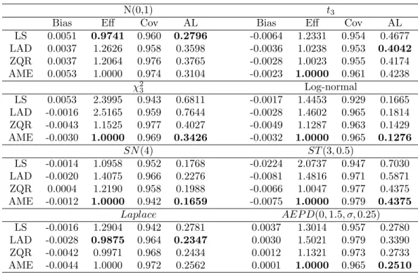
The proposed methodology denoted by AME (adaptive M-estimator) was implemented to analyze each of the simulated data sets, using the techniques outlined in Section 2 and 3. In order to provide a comparison between the proposed methodology and existing techniques, several competing procedures were also implemented. In particular, each data set was analyzed using LS, LAD, and ZQR. The two former techniques are staples among standard data analysis methods, while the latter can be viewed as a generalization of quantile regression which estimates the quantile of interest along with the rest of the model parameters, thus allowing the approach to ”adapt” to the data. In order to estimate standard errors and to construct confidence intervals the standard techniques were used for LS, while bootstrapping techniques withB = 1000 were used for the proposed approach, LAD, and ZQR. It is worthwhile to point out that all of the aforementioned methods attempt to estimate the same slope coefficient (i.e.,β1) in the data generating model above; i.e.,β1is the slope coefficient for the mean and all quantile functions. Thus, this study focuses solely on the results that were obtained from the proposed approach and the three competing techniques for the slope parameter. Table 2.1 provides a summary of the estimators resulting from the proposed procedure, across all considered error distributions. In particular, this summary includes the empirical bias, the relative efficiency of the estimator (i.e., the average estimated standard error of the estimator divided by the average estimated standard error of the proposed estimator), empirical coverage probabilities associated with 95% confidence intervals, and average confidence interval length. From these results, one will notice that the proposed method performs very well; i.e., our estimator exhibits little if any

(24)

Table 2.1: Simulation results summarizing the estimates of the ”slope” coefficient obtained by AME, LS, LAD, and ZQR, for both the AEPD and non-AEPD error distributions. This summary includes the average estimate minus the true value (Bias), relative efficiency (Eff), estimated coverage proba-bility (Cov) associated with 95% confidence intervals, and averaged confidence interval length (AL). Heret3denotes Student’s t-distribution with 3 degrees of freedom;χ23denotes a Chi-square distribu-tion with 3 degrees of freedom;SN(4) denotes a skewed normal distribution with a slant parameter of 4;ST(3,0.5) for skewed t-distribution with 3 degrees of freedom and a skewing parameter of 0.5.

N(0,1) t3

Bias Eff Cov AL Bias Eff Cov AL

LS 0.0051 0.9741 0.960 0.2796 -0.0064 1.2331 0.954 0.4677 LAD 0.0037 1.2626 0.958 0.3598 -0.0036 1.0238 0.953 0.4042 ZQR 0.0037 1.2064 0.976 0.3765 -0.0028 1.0023 0.955 0.4174 AME 0.0053 1.0000 0.974 0.3104 -0.0023 1.0000 0.961 0.4238 χ23 Log-normal LS 0.0053 2.3995 0.943 0.6811 -0.0017 1.4453 0.929 0.1665 LAD -0.0016 2.5165 0.959 0.7644 -0.0028 1.4602 0.965 0.1814 ZQR -0.0043 1.1525 0.977 0.4027 -0.0049 1.1287 0.963 0.1429 AME -0.0030 1.0000 0.969 0.3426 -0.0032 1.0000 0.965 0.1276 SN(4) ST(3,0.5) LS -0.0014 1.0958 0.952 0.1768 -0.0224 2.0737 0.947 0.7030 LAD -0.0020 1.4075 0.966 0.2276 -0.0081 1.4816 0.971 0.5871 ZQR 0.0004 1.2190 0.958 0.1988 -0.0066 1.0047 0.977 0.4375 AME -0.0012 1.0000 0.942 0.1659 -0.0075 1.0000 0.979 0.4375 Laplace AEP D(0,1.5, σ,0.25) LS -0.0016 1.2904 0.942 0.2781 0.0037 1.3014 0.957 0.2780 LAD -0.0028 0.9875 0.964 0.2347 0.0030 1.5021 0.979 0.3390 ZQR -0.0042 0.9971 0.968 0.2434 0.0012 1.1321 0.973 0.2733 AME -0.0044 1.0000 0.972 0.2562 0.0001 1.0000 0.965 0.2510

evidence of bias and the empirical coverage probabilities appear to attain their nominal level. Table 2.1 also provides the same summary for the other three competing regression tech-niques. Unsurprisingly, the same conclusions discussed above can also be drawn for LS, LAD, and ZQR, but differences in performance are apparent. First, under normal (Laplacian) errors the most efficient procedure is LS (LAD), which can be ascertained by examining both the relative efficiency and the average confidence interval length. Note, this finding was expected since LS and LAD result in the MLE under normal and Laplacian errors, respectively. With that being said, one will also note that the estimators resulting from the proposed approach are almost as efficient as the most efficient estimator under normal and Laplacian errors, even though the proposed method is tasked to estimate two additional parameters in these settings. Second, for all other considered error dis-tributions the proposed method provided for the most efficient estimator, with the exception of the setting in which the errors obey a Student’s t-distribution. In some cases the efficiency gains are

(25)

substantial; e.g., under Chi-square errors the proposed estimator is twice as efficient when compared to the the LS and LAD estimators. In general, the proposed approach performed better in terms of estimation efficiency than LS, LAD, and ZQR when the error distribution was asymmetric. More-over, the proposed approach surprisingly outperformed ZQR, which is the most comparable existing technique, in all considered settings. In summary, this simulation study illustrates that the proposed methodology provides reliable estimates across a broad spectrum of potential error distributions, and can provide for more efficient estimates when compared to existing regression methods. Moreover, these gains in estimation efficiency are more dramatic for asymmetric error distributions.

2.4.1

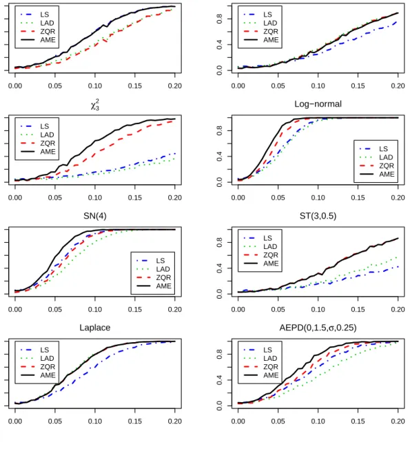
Power of the hypothesis test

In order to investigate other inferential characteristics of the proposed approach, a power analysis was conducted to assess the performance of the proposed methodology when utilized to testH0:β1= 0 versusH1:β16= 0, at theα= 0.05 significance level. Data for this study was generated in the exact same fashion as was described above with a few minor exceptions; i.e., here the slope coefficient is taken to be β1 ∈ {0,0.005, . . . ,0.2}, then for each error distribution and value of β1, m= 1000 independent data sets are generated each consisting ofn= 500 observations. Our approach along with LS, LAD, and ZQR were applied to each of the data sets and the results from these analyses were used to create 95% confidence intervals, as was described in the previous section. Decisions between the null and alternative hypothesis were made based on the confidence intervals in the usual fashion. These results were then used to construct power curves for each of the regression techniques, under each of the considered error distributions.

Figure 2.2provides the empirical power curves for all four regression techniques across all considered error distributions. Again, as one should expect, in the case of Gaussian and Laplacian errors the methods with the most power are LS and LAD, respectively, but the power curve for the proposed approach is practically identical. In contrast, when the error distribution is not normal or Laplace, LS and LAD can suffer from a dramatic loss in power (e.g., Chi-square or skewed t errors) a feature which the proposed approach does not possess. In fact, for skewed distributions one will note that the proposed approach has the most power to detect departures from the null, under all considered configurations. In summary, the findings from this study reinforce the main findings discussed above; i.e., the proposed methodology provides for efficient estimation and reliable inference across a broad spectrum of error distributions.

(26)

Figure 2.2: Empirical power curves obtained under AME, LS, LAD, and ZQR. Heret3denotes Stu-dent’s t-distribution with 3 degrees of freedom;χ2₃denotes a Chi-square distribution with 3 degrees of freedom;SN(4) denotes a skewed normal distribution with a slant parameter of 4; ST(3,0.5) for skewed t-distribution with 3 degrees of freedom and a skewing parameter of 0.5.

0.00 0.05 0.10 0.15 0.20 0.0 0.4 0.8 N(0,1) β1 Empir ical P o w er LS LAD ZQR AME 0.00 0.05 0.10 0.15 0.20 0.0 0.4 0.8 t3 β1 Empir ical P o w er LS LAD ZQR AME 0.00 0.05 0.10 0.15 0.20 0.0 0.4 0.8 χ3 2 β1 Empir ical P o w er LS LAD ZQR AME 0.00 0.05 0.10 0.15 0.20 0.0 0.4 0.8 Log−normal β1 Empir ical P o w er LS LAD ZQR AME 0.00 0.05 0.10 0.15 0.20 0.0 0.4 0.8 SN(4) β1 Empir ical P o w er LS LAD ZQR AME 0.00 0.05 0.10 0.15 0.20 0.0 0.4 0.8 ST(3,0.5) β1 Empir ical P o w er LS LAD ZQR AME 0.00 0.05 0.10 0.15 0.20 0.0 0.4 0.8 Laplace Empir ical P o w er LS LAD ZQR AME 0.00 0.05 0.10 0.15 0.20 0.0 0.4 0.8 AEPD(0,1.5,σ,0.25) Empir ical P o w er LS LAD ZQR AME

(27)

2.5

Data applications

In this section the proposed M-estimator is used to analyze two data sets. These applications further illustrate the useful properties of the proposed regression methodology.

2.5.1

Blood pressure data

The National Health and Nutrition Examination Survey (NHANES) is a Center for Disease Control and Prevention program which was initiated to assess the general health of the populous in the United States. As a part of this study, data is collected from participants via questionnaires and various physical exams, to include laboratory testing. This information is subsequently made publicly available so that researchers may address/explore future medical, environmental, and public health issues that the United States, and more generally the world, may face. One such issue involves the significant number of adults who are affected by high blood pressure. In fact, the World Health Organization (World Health Organization; 2016) estimates that 22% of adults overs the age of 18 have abnormally high blood pressure, equating to approximately 1.2 billion afflicted individuals world wide. Individuals with chronic high blood pressure may develop further sequelae to include aneurysms, coronary artery disease, heart failure, strokes, dementia, kidney failure, etc. (Chobanian et al., 2003). Thus, developing a sound understanding of the relationship that exists between blood pressure and other risk factors is essential to public health.

To this end, the analysis considered herein examines blood pressure data collected on the participants of the NHANES study during the years of 2009-2010, and attempts to relate this response (diastolic blood pressure) to several different risk factors. In particular, the risk factors selected for this study include a binary variable (Food) indicating whether the participant had eaten within the last 30 minutes (with 1 indicating that they had, and 0 otherwise), the average number of cigarettes smoked per day during the past 30 days (Cigarette), the average number of alcoholic drinks consumed per day during the past 12 months (Alcohol), and the participants age (Age). This analysis assumes that a first order linear model is appropriate, and uses the proposed approach as well as LS, LAD, and ZQR to complete model fitting. These techniques were implemented in the exact same fashion as was described in Section3.3. Table 2.2reports the estimated regression coefficients as well as the corresponding standard errors obtained from this analysis.

(28)

Table 2.2: Blood pressure data analysis: Estimated regression coefficients, their estimated standard errors in parenthesis, and the values of the model selection criteria AIC and BIC, resulting from AME, LS, LAD, and ZQR.

Estimate(SE)

Method Food Alcohol Cigarette Age (AIC,BIC) LS -0.481(1.279) 0.452(0.157) -0.001(0.069) 0.473(0.041) (7066.61, 7095.06) LAD 0.170(1.251) 0.430(0.170) -0.024(0.057) 0.385(0.044) (7028.93, 7057.37) ZQR 1.429(1.451) 0.429(0.182) 0.000(0.051) 0.286(0.051) (6985.03, 7018.22) AME 0.675(1.170) 0.405(0.160) 0.004(0.047) 0.316(0.039) (6962.68, 7000.61)

regression methodologies are similar, but differences are apparent. In particular, this analysis finds that age and alcohol are significantly (positively) related to diastolic blood pressure, with the other two covariates being insignificant. The effect estimate associated with alcohol consumption is in agreement across all of the techniques, but the same cannot be said for the age effect. In partic-ular, the proposed method actually renders an age effect estimate that is statistically different (or essentially) than the effect estimate which was obtained by LS. In contrast, the age effect estimates obtained by the proposed approach and ZQR are generally in agreement, this is likely attributable to the fact that both of these techniques are designed to adapt to the asymmetry of the data, which is present in this analysis; e.g., the proposed approach estimated the shape parameter to be ˆα≈1.4 and the skewness parameter to be ˆτ ≈ 0.3, indicating that the error distribution has heavy tails and is right skewed. To further investigate this, Figure 2.3 provides QQ-plots and histograms of the residuals obtained under the four regression methodologies. From Figure 2.3 one would note that LS, LAD, and likely even ZQR would fail basic diagnostic checks. Further, when comparing the standard error estimates of the age effect one will also note that the proposed approach renders a smaller value when compared to LS, LAD and ZQR, which is not surprising given the results discussed in Section 4. Ultimately, in terms of choosing a ”best” model fit in this scenario one could make use of the Akaike Information Criterion (AIC) or the Bayesian Information Criterion (BIC) to select between model fits, noting that the proposed approach holds the other 3 as special cases. Table 2.2provides the values of these model selection criteria for all of the regression techniques, and one will note that both techniques unanimously select the model fit via the proposed approach. In summary, whether based on standard diagnostic procedures, estimator efficiency, or model selection criteria, the proposed approach appears to be the favorable technique for this application.

(29)

Figure 2.3: QQ-plots and histogram of the residuals under AME, LS, LAD, and ZQR for the blood pressure dataset. ● ● ●●●●●●●●●●●● ●●●●●●●●●●●●●●●●●●●●●●●●●●●●●●●●●●●●●●●●●●●●●●●●●●●●●●●●●●●●●●●●●●●●●●●●●●●●●●●●●●●●●●●●●●●●●●●●●●●●●●●●●●●●●●●●●●●●●●●●●●●●●●●●●●●●●●●●●●●●●●●●●●●●●●●●●●●●●●●●●●●●●●●●●●●●●●●●●●●●●●●●●●●●●●●●●●●●●●●●●●●●●●●●●●●●●●●●●●●●●●●●●●●●●●●●●●●●●●●●●●●●●●●●●●●●●●●●●●●●●●●●●●●●●●●●●●●●●●●●●●●●●●●●●●●●●●●●●●●●●●●●●●●●●●●●●●●●●●●●●●●●●●●●●●●●●●●●●●●●●●●●●●●●●●●●●●●●●●●●●●●●●●●●●●●●●●●●●●●●●●●●●●●●●●●●●●●●●●●●●●●●●●●●●●●●●●●●●●●●●●●●●●●●●●●●●●●●●●●●●●●●●●●●●●●●●●●●●●●●●●●●●●●●●●●●●●●●●●●●●●●●●●●●●●●●●●●●●●●●●●●●●●●●●●●●●●●●●●●●●●●●●●●●●●●●●●●●●●●●●●●●●●●●●●●●●●●●●●●●●●●●●●●●●●●●●●●●●●●●●●●●●●●●●●●●●●●●●●●●●●●●●●●●●●●●●●●●●●●●●●●●●●●●●●●●●●●●●●●●●●●●●●●●●●●●●●●●●●●●●●●●●●●●●●●●●●●●●●●●●●●●●●●●●●●●●●●●●●●●●●●●●●●●●●●●●●●●●●●●●●●●●●●●●●●●●●●●●●●●●●●●●●●●●●●●●●●●●●●●●●●●●●●●●●●●●●●●●●●●●●●●●●●●●●●●●●●●●●●●●●●●●●●●●●●●●●●●●●●●●●●●●●●● ●● ● ● −40 −20 0 20 40 −40 0 40 80 LS theoretical quantiles empir ical quantiles LS Residuals Density −40 −20 0 20 40 60 80 0.00 0.02 0.04 ● ● ● ●●●●●●●●● ●●●●●●●●●●●●●●●●●●●●●●●●●●●●●●●●●●●●●●●●●●●●●●●●●●●●●●●●●●●●●●●●●●●●●●●●●●●●●●●●●●●●●●●●●●●●●●●●●●●●●●●●●●●●●●●●●●●●●●●●●●●●●●●●●●●●●●●●●●●●●●●●●●●●●●●●●●●●●●●●●●●●●●●●●●●●●●●●●●●●●●●●●●●●●●●●●●●●●●●●●●●●●●●●●●●●●●●●●●●●●●●●●●●●●●●●●●●●●●●●●●●●●●●●●●●●●●●●●●●●●●●●●●●●●●●●●●●●●●●●●●●●●●●●●●●●●●●●●●●●●●●●●●●●●●●●●●●●●●●●●●●●●●●●●●●●●●●●●●●●●●●●●●●●●●●●●●●●●●●●●●●●●●●●●●●●●●●●●●●●●●●●●●●●●●●●●●●●●●●●●●●●●●●●●●●●●●●●●●●●●●●●●●●●●●●●●●●●●●●●●●●●●●●●●●●●●●●●●●●●●●●●●●●●●●●●●●●●●●●●●●●●●●●●●●●●●●●●●●●●●●●●●●●●●●●●●●●●●●●●●●●●●●●●●●●●●●●●●●●●●●●●●●●●●●●●●●●●●●●●●●●●●●●●●●●●●●●●●●●●●●●●●●●●●●●●●●●●●●●●●●●●●●●●●●●●●●●●●●●●●●●●●●●●●●●●●●●●●●●●●●●●●●●●●●●●●●●●●●●●●●●●●●●●●●●●●●●●●●●●●●●●●●●●●●●●●●●●●●●●●●●●●●●●●●●●●●●●●●●●●●●●●●●●●●●●●●●●●●●●●●●●●●●●●●●●●●●●●●●●●●●●●●●●●●●●●●●●●●●●●●●●●●●●●●●●●●●●●●●●●●●●●●●●●●●●●●●●●●●●●●●●●●●● ●● ● ● ● ● −50 0 50 −20 20 60 LAD theoretical quantiles empir ical quantiles LAD Residuals Density −40 −20 0 20 40 60 80 0.00 0.02 0.04 ● ●●●●●●●●● ●●●●●●●●●●●●●●●●●●●●●●●●●●●●●●●●●●●●●●●●●●●●●●●●●●●●●●●●●●●●●●●●●●●●●●●●●●●●●●●●●●●●●●●●●●●●●●●●●●●●●●●●●●●●●●●●●●●●●●●●●●●●●●●●●●●●●●●●●●●●●●●●●●●●●●●●●●●●●●●●●●●●●●●●●●●●●●●●●●●●●●●●●●●●●●●●●●●●●●●●●●●●●●●●●●●●●●●●●●●●●●●●●●●●●●●●●●●●●●●●●●●●●●●●●●●●●●●●●●●●●●●●●●●●●●●●●●●●●●●●●●●●●●●●●●●●●●●●●●●●●●●●●●●●●●●●●●●●●●●●●●●●●●●●●●●●●●●●●●●●●●●●●●●●●●●●●●●●●●●●●●●●●●●●●●●●●●●●●●●●●●●●●●●●●●●●●●●●●●●●●●●●●●●●●●●●●●●●●●●●●●●●●●●●●●●●●●●●●●●●●●●●●●●●●●●●●●●●●●●●●●●●●●●●●●●●●●●●●●●●●●●●●●●●●●●●●●●●●●●●●●●●●●●●●●●●●●●●●●●●●●●●●●●●●●●●●●●●●●●●●●●●●●●●●●●●●●●●●●●●●●●●●●●●●●●●●●●●●●●●●●●●●●●●●●●●●●●●●●●●●●●●●●●●●●●●●●●●●●●●●●●●●●●●●●●●●●●●●●●●●●●●●●●●●●●●●●●●●●●●●●●●●●●●●●●●●●●●●●●●●●●●●●●●●●●●●●●●●●●●●●●●●●●●●●●●●●●●●●●●●●●●●●●●●●●●●●●●●●●●●●●●●●●●●●●●●●●●●●●●●●●●●●●●●●●●●●●●●●●●●●●●●●●●●●●●●●●●●●●●●●●●●●●●●●●●●●●●●●●●●●●●●●●●● ●●● ● ● ● ● 0 50 100 −20 20 60 ZQR theoretical quantiles empir ical quantiles ZQR Residuals Density −40 −20 0 20 40 60 80 0.00 0.02 0.04 ● ●●●●●●●●●●● ●●●●●●●●●●●●●●●●●●●●●●●●●●●●●●●●●●●●●●●●●●●●●●●●●●●●●●●●●●●●●●●●●●●●●●●●●●●●●●●●●●●●●●●●●●●●●●●●●●●●●●●●●●●●●●●●●●●●●●●●●●●●●●●●●●●●●●●●●●●●●●●●●●●●●●●●●●●●●●●●●●●●●●●●●●●●●●●●●●●●●●●●●●●●●●●●●●●●●●●●●●●●●●●●●●●●●●●●●●●●●●●●●●●●●●●●●●●●●●●●●●●●●●●●●●●●●●●●●●●●●●●●●●●●●●●●●●●●●●●●●●●●●●●●●●●●●●●●●●●●●●●●●●●●●●●●●●●●●●●●●●●●●●●●●●●●●●●●●●●●●●●●●●●●●●●●●●●●●●●●●●●●●●●●●●●●●●●●●●●●●●●●●●●●●●●●●●●●●●●●●●●●●●●●●●●●●●●●●●●●●●●●●●●●●●●●●●●●●●●●●●●●●●●●●●●●●●●●●●●●●●●●●●●●●●●●●●●●●●●●●●●●●●●●●●●●●●●●●●●●●●●●●●●●●●●●●●●●●●●●●●●●●●●●●●●●●●●●●●●●●●●●●●●●●●●●●●●●●●●●●●●●●●●●●●●●●●●●●●●●●●●●●●●●●●●●●●●●●●●●●●●●●●●●●●●●●●●●●●●●●●●●●●●●●●●●●●●●●●●●●●●●●●●●●●●●●●●●●●●●●●●●●●●●●●●●●●●●●●●●●●●●●●●●●●●●●●●●●●●●●●●●●●●●●●●●●●●●●●●●●●●●●●●●●●●●●●●●●●●●●●●●●●●●●●●●●●●●●●●●●●●●●●●●●●●●●●●●●●●●●●●●●●●●●●●●●●●●●●●●●●●●●●●●●●●●●●●●●●●●●●●●●●●● ●●● ● ● ● −20 0 20 40 60 80 −20 20 60 AME empir ical quantiles AME Density −40 −20 0 20 40 60 80 0.00 0.02 0.04

(30)

2.5.2

Miscarriage data

The Collaborative Perinatal Project (CPP) was a longitudinal study, conducted from 1957 to 1974, which was aimed at assessing multiple aspects of maternal and child health (Hardy, 2003). Even though this study was conducted half a century ago, the information collected still constitutes an important resource for biomedical research in many areas of perinatology and pediatrics. For ex-ample, in 2007 a nested case-control study which examined whether circulating levels of chemokines were related to miscarriage risk was conducted using (n= 745) stored serum samples collected as a part of the original CPP study, for further details seeWhitcomb et al. (2007). In particular, this study focused on monocyte chemotactic protein-1 (MCP1), which is a cytokine that is located on chromosome 17 in the human genome and is believed to have a pregnancy regulatory function, for further details seeWood (1997). The cases (controls) in the study were participants who had (not) experienced a spontaneous miscarriage, and cases were matched with controls based on gestational age. In addition to the measured MCP1 levels, several other variables were collected on each partic-ipant; i.e., age, race (with 1 denoting Africa American, and 0 otherwise)), smoke (with 1 denoting that the participant had smoked before and 0 otherwise) and miscarriage status (with 1 denoting that miscarriage had been experienced, and 0 otherwise).

In this analysis, the measured MCP1 level is considered to be the response variable and all other variables are treated as covariates. A full linear model consisting of all first order terms, as well as all pairwise interactions, is assumed and best subset model selection is implemented using BIC as the criteria. The proposed approach was used to fit all possible models, including models where (α, τ) were set to be (2,0.5), (1,0.5), and (1, τ), which are equivalent to implementing LS, LAD, and ZQR, respectively. Model fitting was conducted in the exact same fashion as was described in Section3.3. This process identified an intercept only model for LS, a model consisting of race as the only covariate for ZQR, and a first order model consisting of both age and race as covariates for LAD and AME, with BIC values of 431.28, -395.51, -822.02, and -937.55 for LS, LAD, ZQR, and AME, respectively. From these results, one will note that important relationships will potentially be missed when the appropriate regression methodology is not used. In particular, this study illustrates that the best model chosen under these existing procedures may differ from the best model chosen under the proposed approach. When one considers the model selection process described above, it would be natural to place more faith in the results that were obtained under the proposed approach. This

(31)

assertion is based on two primary facts. First, the proposed procedure holds the other competing procedures as special cases, thus the analysis described above should be viewed as a much more in depth model selection process which evaluates whether it is more reasonable to view α and τ as being fixed (with known value) or as unknown parameters. Second, of the considered techniques the proposed procedure has the ability to more aptly adapt to the underlying error structure, and is therefore able to render a more reliable analysis.

2.6

Conclusions

This work has developed a general robust regression methodology, which was inspired by the asym-metric exponential power distribution. In particular, the proposed methodology is robust with respect to the underlying error structure, thus rendering reliable estimation and inference across a broad spectrum of error distributions, even in the case of heavy tails and/or asymmetry. This is made possible by the fact that the loss function is chosen in a data adaptive fashion, during the esti-mation process, thus capturing the shape and skewness of the underlying distribution of the errors. The asymptotic properties of the proposed estimator are established. Through an extensive Monte Carlo simulation study, the proposed approach was shown to perform as well if not better than several existing techniques. In particular, these studies show that the proposed method generally performs better than these existing techniques when the error distribution is heavy-tailed and/or skewed. The strengths of the proposed method were further exhibited through the analysis of two motivating data sets. To further disseminate this work, code (written in R) which implements the proposed methodology has been prepared and is available upon request.

Acknowledgments

This work was partially supported by Grant R01 AI121351 from the National Institutes of Health.

Appendix

The regularity conditions under which consistency and asymptotic normality of the proposed M-estimator and the bootstrapped M-estimator can be established are provided below.

(32)

A1: {(xi, yi), i= 1, . . . , n}is an i.i.d. sequence of random variables.

A2: The conditional cumulative distribution function of y|x is absolutely continuous and has a positive density denoted byf∗(·|·).

A3: The parameter space Θ⊂Ξ≡ {θ|α >0, σ >0, τ ∈(0,1), βi∈R,∀i}, and Θ is a compact set.

A4: There exists a unique θ0 ∈ Θ such that E{lnf(y|x,θ)} is maximized and has nonsingular second derivative atθ0.

A5: kn−1Pn

i=1ψ(yi,xi,θˆ)k=op(n−1/2).

A6: There exists a δ such that 0 < δ < α−1, E ||2 ¯α+4δ

< ∞, and E |xj|2 ¯α+4δ

< ∞, for

j = 1, ..., p, where α and ¯α denote the infimum and supremum of the set of all α in Θ, respectively.

A7: V1θ0 andV2θ0 exist and are finite,V1θ0 is positive definite, andV2θ0 is invertible.

Conditions A1-A5 and A7 are common in the literature, see Huber (1967), Huber and Ronchetti (2009),Koenker (2005), andBera et al. (2016). Condition A2 restricts the conditional distribution of the dependent variable and Condition A7 is assumed so that the asymptotic variance of the estimator exists and is finite. Condition A4 ensures identifiability and existence of a unique solution. Condition A5 is used to ensure that the derivative of the loss function evaluated at ˆθis “nearly-zero”. Condition A6 restricts the absolute moments on the conditional distribution ofy|x and each covariate xj in order to ensure the asymptotic behavior of the proposed estimator.

The consistency and asymptotic normality of the proposed estimator and the bootstrapped estimator are established by verifying the conditions inHuber and Ronchetti (2009)(page 127 for consistency and Theorem 6.6 as well as its corollary for normality) and Arcones and Gin´e (1992) (page 42), respectively. The arguments to verify these assumptions are similar to those inZhu (2009) and Bera et al. (2016), and the details of these arguments are available from the corresponding author.

(33)

Chapter 3

Adaptive Penalized Quantile

Regression for Variable Selection

3.1

Introduction

Suppose that (x0_i, yi)ni=1 represents an independent and identically distributed (iid) sample which is assumed to follow a joint distribution g(y,x), with y being a response variable and x being a

p-dimensional covariate vector. In many settings, the conditional mean of y given x is assumed to be β0 +x0β. In general, some of the covariates are important and others are not; in some studies e.g. genomics/genetics it is the case that most are unimportant. In these situations, variable selection techniques can be used to attempt to identify important variables, which is equivalent to identify which regression coefficients are non-zero. In general, two evaluation metrics are concerned: the mean squared error (MSE) or the mean absolute error (MAE) of the regression coefficients estimates to measure the accuracy of the estimates and the average number of correctly specified and mis-specified unimportant covariates to assess the variable selection performance. Both metrics are related to the accuracy of prediction that takes both the bias and the variability of the estimates into account. The following literature review gives a brief introduction of several methods which have been proposed to perform regression coefficients estimation and variable selection simultaneously.

In practice, the true density g(y,x) is rarely known, so a parametric model fθ(y,x) is

(34)

models, where part ofθis allowed to be any sub-vector of apdimensional “slope” coefficient vector with coefficients corresponds to covariates being potentially related to the response, then a working model class is constructed which consists of a set of competing models that is denoted by{Mm:m= 1,· · · ,2p_{}. If the true model belongs to the assumed model class, from the perspective of} Kullback-Leibler (KL) divergence defined in (2.5),Akaike (1974)shows that up to a constant, the estimated KL divergence for model Mm can be asymptotically expanded as −ln(ˆθm) +Pp_j₌₁I(ˆθm,j 6= 0), where ln(ˆθm) is the log-likelihood function for model Mm evaluated at the maximum likelihood estimate ˆθm for m= 1,· · ·,2p_{, and} _{Schwarz (1978)}_{proposes the BIC criterion from the Bayesian} principle which yields−ln(ˆθm) + ln(n)/2P

p

j=1I(ˆθm,j 6= 0) as the criterion for model selection. Both AIC and BIC choose a model that minimizes the penalized likelihood; i.e.,

arg min

θ

−ln(θ) +λ||θ||0, (3.1) for different values of λ, where || · ||0 is called the L0 norm that counts the number of non-zero components. Many traditional methods can amount to penalized least squares (LS) methods with different choices ofλwhen the Normal likelihood in (3.1) is used. This includes Mallow’sCpstatistics inMallows (1973)corresponds toλ= 1 and the adjustedR2_{is approximately equivalent to}_λ_{= 1}_/_2. (See details inFan and Lv, 2010). (3.1) can be solved whenpis rather small via best subsets, but aspincreases this problem quickly becomes unsolvable. In case when the number of covariatespis comparable to or larger than the sample sizen, the computation ofL0regularization is infeasible.

Tibshirani (1996)proposed the least absolute shrinkage and selection operator (Lasso) that is defined as follows, arg min β0∈R,β∈Rp 1 n n X i=1 (yi−β0−x0iβ) 2 _{subject to} p X j=1 |βj| ≤t, (3.2) here t is a tunning parameter. If t is greater than or equal to theL1 norm of the OLS estimator, then (3.2) is equivalent to the unconstrained problem, which yields the OLS estimator. For smaller values oft, Lasso shrinks the estimated coefficients toward the origin, and typically sets some of the coefficients to be identically equal to zero. The optimization problem described in (3.2) has its dual

(35)

form which is given by arg min β0∈R,β∈Rp 1 n n X i=1 (yi−β0−x0iβ) 2₊_λ p X j=1 |βj|. (3.3) Problems (3.2) and (3.3) are equivalent; that is, for a givenλ≥0, there exists at≥0 such that the two problems share the sa