An Introduction to Physically Based Modeling: Constrained Dynamics

An Introduction to Physically Based Modeling:

Constrained Dynamics

Andrew Witkin

Robotics Institute

Carnegie Mellon University

Please note: This document is



1997 by Andrew Witkin. This chapter may be

freely duplicated and distributed so long as no consideration is received in return,

and this copyright notice remains intact.

Constrained Dynamics

School of Computer Science Carnegie Mellon University

1

Beyond penalty methods

The idea of constrained particle dynamics is that our description of the system includes not only particles and forces, but restrictions on the way the particles are permitted to move. For example, we might constrain a particle to move along a specified curve, or require two particles to remain a specified distance apart. The problem of constrained dynamics is to make the particles obey Newton’s laws, and at the same time obey the geometric constraints.

As we learned earlier, energy functions provide a sloppy, approximate constraint mechanism. A spring with rest length r makes the particles it connects “want” to be distance r apart. How-ever, the spring force competes with all other forces acting on the particles—gravity, other springs, forces applied by the user, etc. The constraint can only win this tug-of-war if its spring constant is large enough to overpower all competing influences, so that very small displacements induce large restoring forces. As we saw in the last section, this is really no solution because it gives rise to stiff differential equations which are all but numerically intractible. The use of extra energy terms to impose constraints is known as the penalty method. If we want both accurate constraints and numerical tractibility, then penalty methods will not fill the bill.

Penalty constraints work, to the extent they do, because the restoring forces cancel applied forces that would otherwise break the constraints. The fundamental difficulty with penalty constraints is that the applied forces and restoring forces communicate only indirectly, through displacements. In effect, the displacements produced by applied forces act as signals that tell the constraint what restoring force is required. This is not a good communication mechanism because it is impossible to acheive accuracy without stiffness.

The basic approach to avoiding this problem is to directly calculate the forces required to main-tain the constraints, rather than relying on displacements and restoring forces to do the job. The job of these constraint forces is to cancel just those parts of the applied forces that act against the con-straints. Since forces influence acceleration, this means specifically that the constraint forces must convert the particles’ accelerations into “legal” accelerations that are consistent with the constraints.

2

A bead on a wire

We introduce the approach using the simple example of a 2D particle constrained to move on the unit circle. We can express the constraint by writing a scalar behavior function, as we did in Chapter C to create energy functions,

C(x)= 1

Maintaining Constraints Differentially

C = 0

C = 0

C = 0

Point-on-circle constraint:

C = 0 legal position

C = 0 legal velocity

C = 0 legal acceleration

C =

(

x

⋅

x - 1

)

Add in a constraint force that

ensures legal acceleration.

Figure 1: If the initial position and velocity are consistent with the constraints, then the constraint can be maintained by ensuring that the acceleration is always legal thereafter.

so that the legal positions of x are all those that satisfy C(x) = 0. The function C is an implicit

function for the constraint. If x is a legal position, then the legal velocities are all those that satisfy ˙

C=x· ˙x=0. (2)

In turn, the legal accelerations are all those that satisfy

¨

C = ¨x·x+ ˙x· ˙x=0. (3) If we start out with a legal position and velocity, then to maintain the constraint, in principal, we need only ensure that equation 3 is satisfied at every instant thereafter. See figure 1 The particle’s acceleration is

¨

x= f+ ˆf

m , (4)

where f is the given applied force, andˆf is the as yet unknown constraint force. Substituting forx in¨ equation 3 gives ¨ C = f+ ˆf m ·x+ ˙x· ˙x=0, (5) or ˆ f·x= −f·x−mx˙ · ˙x. (6)

2.1 The principal of virtual work

We have only one equation and two unknowns—the two components of ˆf—so we cannot solve for the constraint force without an additional condition. We get that condition by requiring that

the constraint force never add energy to nor remove energy from the system, i.e. the constraint is passive and lossless. The kinetic energy is

T = m

2x˙· ˙x, and its time derivative is

˙

T =mx¨· ˙x=mf· ˙x+mˆf· ˙x,

which is the work done by f andˆf. Requiring that the constraint not change the energy means that the last term must be zero, i.e. that the constraint force does no work. A subtle point is that we are enjoining the constraint force from ever doing work, rather than saying that it happens not to be at the moment. We therefore require thetˆf· ˙x vanish for every legalx, i.e.˙

ˆ

f· ˙x=0,∀˙x|x· ˙x=0.

This condition simply states thatx must point in the direction of x, so we can rewrite the constraintˆ force as

ˆ

f=λx,

whereλis an unknown scalar. Substituting forˆf in equation 6, and solving forλgives

λ= −f·x−mx˙· ˙x

x·x . (7)

Having solved forλ, we calculateˆf=λx, thenx¨ =(ˆf+f)/m, and proceed with the simulation in

the usual way.

In its general form, the condition we imposed onˆf is known as the principal of virtual work.[2] See figure 2 for an illustration.

2.2 Feedback

If we were solving the differential equation exactly, this procedure would keep the particle exactly on the unit circle, provided we began with valid initial conditions. In practice, we know that nu-merical solutions to ODE’s drift. We must add an extra feedback term to prevent this nunu-merical drift from accumulating, turning the circle into an outward spiral. The feedback term can be just a damped spring force, pulling the particle back onto a unit circle. The feedback force needs to be added in after the constraint force calculation, or else the constraint force will dutifully cancel it! We will discuss feedback in more detail in the next section.

2.3 Geometric Interpretation

When the system is at rest, the constraint force given in equation 7 reduces to

ˆ

f= −f·x

x·xx, (8)

which has clear geometric interpretation as the vector that orthogonally projects f onto the circle’s tangent. This interpretation makes intuitive sense because the force component that is removed by this projection is the component that points out of the legal motion direction. The orthogonality of the projection also makes sense, because it ensures that the particle will not experience gratuitous accelerations in the allowed direction of motion.

Constraint Forces

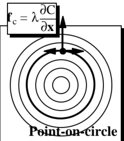
Point-on-circle

f

=

λ∂

C

∂

x

• Restrict constraint

force to the normal

direction.

• Orthogonal to all legal

displacements.

• No work, no energy

gain or loss.

• One DOF:

λ

Figure 2: In the case of a point-on-circle constraint, the principle of virtual work simply requires the constraint force to lie in a direction normal to the circle.

Whenx is nonzero, we unfortunately lose this simple geometric picture, but we can still interpret˙ the addition of the constraint force as a projection. Rather than a force projection, it is the projection of the acceleration onto the set of legal accelerations. The velocity-dependent term in equation 7 ensures that the curvature of the particle’s trajectory matches that of the circle. some effort, we could try to regain the geometric picture by visualizing a projection in phase space, but this is hardly worth the trouble.

3

The general case

In the last section we derived the constraint force expression for a single particle subject to a single scalar constraint. Our goal in this section is to extend this special case to the general one of a whole system of particles, collectively subjected to a number of constraints. The derivation follows the more detailed one presented in [5].

The key to making this a managable task is to adopt a uniform, monolithic view, much as we do in solving ODEs. Rather than considering each particle separately, we lump their positions into a single state vector, which we will call q.Unlike the phase-space vector that we hand to the solver, this one contains positions only, not velocities,so, in 3D, it has length 3n.

To collapse all the particles’ equations of motion into one global equation, we next define a mass

matrix, M, whose diagonal elements are the particles’ masses, and whose off-diagonal elements are

zero. The diagonal mass matrix for n 3D points is a 3n×3n matrix whose diagonal elements are [m1,m1,m1,m2,m2,m2, . . . ,mn,mn,mn]. implementation, a diagonal matrix may be represented

as a vector. Multiplication of a vector by the matrix is then just element-by-element multiplication. The inverse of a diagonal matrix is just the element-by-element reciprocal.

Finally, we concatenate the forces on all the particles, just as we do the positions, to create a global force vector, which we denote by Q. Now we can write the global equation governing the particle system as

¨

q=WQ, where W is the inverse of M.

We will also use global notation for the constraints, concatenating all the scalar constraint func-tions to form a single vector function C(q). If we have n 3D particles, subject to m scalar con-straints, then the output of this global constraint function is an m-vector, and its input is a 3n-vector. At this point, you may well be wondering how all this global notation will ever actually apply to a real network of particles and constraints. This is an example of just the same kind of duality that we encountered in applying ODE solvers to mass-and-spring models. On the one hand, we want to build particle-and-constraint models as networks of distinct interacting objects. On the other, we want to allow the code that calculates constraint forces to act as if the system on which it operates really were a structureless monolith, just as an ODE solver does. Soon, we will show very concretely how this dual view can be maintained.

As in the point-on-circle example, we assume that the configuration q and the velocityq are˙ both initially legal, i.e. that C= ˙C=0. Then our problem is to solve for a constraint forceQ that,ˆ added to the applied force Q, guarantees thatC¨ =0.

To do this, we will need to take derivatives of C. In the previous section, we had a specific algebraic expression for the constraint function, so we were able to derive expressions for their derivatives as well. Now, since we are regarding C as an anonymous function of state, we will be writing derivatives generically, using expressions such as ∂_∂C_q. To keep things down to earth, you should think of expressions such as these, as well as C itself, as things we are able to evaluate numerically by invoking functions.1

By the chain rule,

˙

C= ∂C

∂qq˙.

The matrix∂C/∂q is called the Jacobian of C. We will denote it henceforward by J. Differentiating again w.r.t. time gives

¨

C= ˙Jq˙ +Jq¨.

The quantityJ, the time derivative of the Jacobian, might be a little puzzling. By the chain rule we˙ could write it as J˙ = ∂J/∂qq˙.However, taking the derivative of a matrix w.r.t. a vector yields a rank 3 tensor (essentially, a 3D array). We can avoid introducing this new kind of object by writing, equivalentlyJ˙ =∂C˙/∂q.Assuming we have an expression forC, this entails only differentiating a˙ vector expression w.r.t. a vector, which is less menacing.

Next, we use the system’s equations of motion to replaceq by a force expression, giving¨

¨

C= ˙Jq˙ +JW(Q+ ˆQ). SettingC to zero and re-arranging gives¨

JWQˆ − ˙Jq˙ −JWQ, (9)

1_{Speaking of derivatives, it is important to understand what a quantity such as∂C/∂q is. Since both C and q are}

vectors, the derivative of one with respect to the other is a matrix, obtained by taking the scalar derivative of each component of C w.r.t. each component of q.

which is the counterpart, in general form, to equation 7. As in the point-on-circle example, we have more unknowns than equations, and once again we introduce the principle of virtual work. The legal velocities (i.e. the ones that don’t change C) are all the ones that satisfy Jx˙ = 0. To ensure that the constraint force does no work, we therefore require that

ˆ

Q· ˙x=0, ∀˙x|Jx˙ =0.

All and only vectorsQ that satisfy this requirement can be expressed in the formˆ

ˆ

Q=JTλ, whereλis a vector with the dimension of C.

To understand what this expression means, it helps to regard the matrix J as a collection of vec-tors, each of which is the gradient of one of the scalar constraint functions comprising C. Since our fundamental requirement is that C=0, these gradients are normals to the constraint hypersurfaces, representing the state-space directions in which the system is not permitted to move. The vectors that have the form JTλare the linear combinations of these gradient vectors, and hence span exactly the set of prohibited directions. Restricting the constraint force to this set ensures that its dot prod-uct with any legal displacement of the system will be zero, which is exactly what the principle of virtual work demands.

In matrix parlance, the set of vectors JTλ is known as the null space complement of J. The

null space of J is the set of vectors v that satisfy Jv = 0. The null space vectors are the legal displacements, while the null space complement vectors are the prohibited ones.

The components of λare known as Lagrange multipliers. These quantities, which determine how much of each constraint gradient is mixed into the constraint force, are the unknowns for which we must solve. To do so, we replaceQ by Jˆ Tλin equation 9, which gives

JWJTλ= −˙Jq˙ −JWQ, (10)

which is a matrix equation in which all butλare known. The matrix JWJT is a square matrix with the dimensions of C. Onceλis obtained, it is multiplied by JT to obtainQ, which is added to theˆ applied force before calculating acceleration.

We already noted the need for a feedback term to prevent the accumulation of numerical drift. This term can be incorporated directly into the constraint force calculation. Instead of solving for

¨

C=0, as we did above, we solve for

¨

C= −ksC−kdC˙,

where ks and kd are spring and damping constants. By adding this term, we make the constraint

force perform the extra function of returning, with damping, to a valid state should drift occur. The final constraint force equation, with feedback, is

JWJTλ= −˙Jq˙ −JWQ−ksC−kdC˙. (11)

The values assigned to ksand kd are not critical, since this term only plays the relatively

4

Tinkertoys: Implementing Constrained Particle Dynamics

The general formula of equation 11 is just a skeleton. To actually simulate anything, a specific constraint function C(q) must be provided, in a form that lets us evaluate the function itself and its various derivatives. One way to flesh out the skeleton would be to write down an expression for such a function, symbolically take the required derivatives, substitute these expressions into equation 11 and, after simplifying and massaging the resulting mess, write code that performs the numerical evaluations required for a simulation. This is essentially what we did in section 2, but only for a trivially simple example. As an exercise, you might try working through a somewhat more complicated example, say a double pendulum. If you actually do try it, you will probably be able to carry it through to a working implementation, but it will be readily apparent that this derive-and-implement methodology does not scale up!

Instead of hand-deriving and hand-coding models, we want to build models interactively by snapping the pieces together, drawing freely from a set of useful pre-defined constraints, such as distance and point-on-curve constraints. The main problem we must solve to acheive this goal is to evaluate the global matrices and vectors that comprise equation 11. The evaluations must be quick, and also dynamic in the sense that we can freely change the structure of the model on the fly. Naturally, we want constraints to be modular just as forces are.

In this section we describe an architecture for constrained particle dynamics simulation that meets these objectives. The approach is to represent individual constraints using objects similar to those that represent forces. Each constraint object is responsible for evaluating the constraint function it represents, and also that functions derivatives. These evaluations produce fragments of the vectors and matrices comprising equation 11. The fragments are then combined dynamically by the constrained particle system.

4.1 The constrained simulation loop

The machinery required to support constraints fits neatly into our basic particle system architecture. From the standpoint of the ODE solver, the main job of the particle system, in both the unconstrained and constrained case, is to perform derivative evaluations. The sequence of steps that the particle system must perform to evaluate the derivative is nearly the same, with one important addition: calculating the constraint force. This is how the extra step fits in:

1. Clear forces: zero each particle’s force accumulator.

2. Calculate forces: loop over all force objects, allowing each to add forces to the particles it influences.

3. Calculate constraint forces: On completion of the previous step, each particle’s force accu-mulator contains the total force on that particle. In this step, the global equation 11 is set up and solved, yielding a constraint force on each particle, which is added into the applied force. 4. Calculate the derivative: Divide force by mass to get acceleration, and gather the derivatives

into a global vector for the solver.

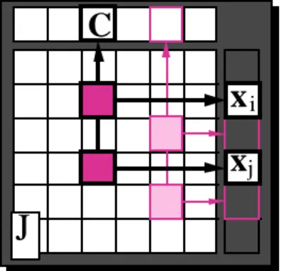
Matrix Block Structure

C

x

x

J

• Each constraint

contributes one or more

blocks to the matrix.

• Sparsity: many empty

blocks.

• Modularity: let each

constraint compute its

own blocks.

Figure 3: The block-sparse Jacobian matrix. The constraints are shown above, and the particles along the right side. Each constraint/particle pair corresponds to a block in the matrix. A block is non-zero only if the constraint depends on the particles. Here, we show a binary constraint, such as a distance constraint, that connects two particles. The two shaded blocks are that constraint’s only contributions to the sparse Jacobian.

4.2 Block-structured matrices

Each individual constraint contributes a slice to the global constraint vector C, just as each particle contributes a slice to the global state vector q. In addition to a list of particles, and a list of forces, a constrained particle system must also maintain a list of constraints. Evaluating the global vectors such as C andC is straightforward, assuming that each constraint points to a function that performs˙ its own portion of these evaluations. We simply loop over the constraints, invoking the functions, and placing the results in the global vectors with appropriate offsets. This is essentially the same gather operation that we use for communication with the ODE solver.

The main new ingredient is that we must evaluate global matrices as well as vectors. Whereas constraints and particles each occupy a slice of their respective global vectors, each

constraint-particle pair occupies a block of the global derivative matrix. The vector slice that is “owned” by

a constraint can be described by an offset and a length, say i and ilengt h. Similarly, a particle’s global station can be described by j and jlengt h. While jlengt h is always the dimension of the space that the particles live in, ilengt h may vary from constraint to constraint. The derivative of a constraint with respect to a particle occupies an ilengt h× jlengt h block of the Jacobian matrix J,

with originn at position(i, j). See figure 3.

A typical constraint influences at most just a few particles. The value of the constraint function depends on only these particles; its derivative with respect to all other particles is zero. This means that the matrices J andJ are typically very sparse. Of the n blocks per constraint in an n-particle˙ system, a unary constraint contributes only one non-zero block, a binary one two non-zero blocks,

etc. Given this structure, a natural way to represent the sparse matrices is by lists of the non-zero blocks. In this scheme, each matrix block is represented by a structure that specifies the block’s origin, (i, j), and dimensions, (ilengt h, jlengt h), and that contains an ilengt h× jlengt h float

array holding the block’s data, e.g.

struct{ int i; int j; int ilength; int jlength; float *data; };

To support constrained particle dynamics using block-sparse matrices, as we will soon see, we must implement only two operations: matrix times vector, and matrix-transpose times vector. Both are simple operations, looping over the matrix blocks, and performing an ordinary matrix multiplication for each block, using the block’s i and j as offsets into the destination and source vectors.

4.3 Building the matrices

In addition to holding lists of particles and forces, the constrained particle system will hold a list of constraints, block-sparse matrices to represent J andJ, and vectors to hold C,˙ C, etc. The structures˙ that represent the constraints may be similar in many respects to the structures we use to represent simple forces, i.e. they point to the particles on which they depend and they point to functions that perform their type-specific operations.

When a constraint is instantiated, matrix blocks must be created for each particle on which the constraint depends, and the blocks must be added to the global matrices. Since the number and shape of blocks involved varies with the constraint type, this initialization may be handled by the constraint in a type-specific way. Thereafter, the constraint must be able to evaluate its portions of the vectors C andC, and of the matrices J and˙ J. The results of the matrix evaluations are placed in˙ the matrix blocks that were created by the constraint on initialization.

All the required global quantities can then be computed simply by looping over the constraints, and invoking the functions that perform these evaluations.

4.4 Solving the linear system

The solution of sparse linear systems is a field unto itself. Of the many available options, we give one that is simple and readily available. A matrix equation of the form Mx = b may be solved

iteratively by finding a vector x that minimizes(Mx−b)·(Mx−b).A conjugate gradient algorithm that solves this problem is given in Numerical Recipes [4], Chapter 2. The conjugate gradient algorithm offers the advantage that it gives a least-squares solution for over-determined systems, and tolerates redundant constraints. The solver takes as arguments two routines which contitute its only access the matrix: vector-times-matrix, and vector-transpose-times matrix. Sparsity is exploited by implementing these routines efficiently. The routine requires O(n)iterations to solve an n×n matrix, and the cost of each iteration is O(m), where m is the number of non-zero entries in the matrix.

The matrix of equation 11 is JWJT, where J is block-sparse and W is diagonal. We need never actually calculate the matrix. Instead we need only calculate JWJTx, given a vector x. We do this by calculating JTx, using the block-sparse matrix-transpose multiply routine described above, then performing an element-by-element multiplication of the result by the vector representing the diag-onal W. Finally, the resulting vector is multiplied by J. Since the compound matrix is symmetric, we do not need a separate function for multiplication by the transpose.

Evaluating the right hand side vector of equation 11 is a straightforward application of the block-sparse matrix routines, and standard vector operations.

Finally, once the linear system has been solved, the vectorλis multiplied by JT to produce the global constraint force vectorQ, which is then scattered into the particles’ force accumulator.ˆ

4.5 Summary

To introduce constraints into a particle system simulation, we add the additional step of constraint force calculation to the derivative evaluation operation. After the ordinary applied forces have been calculated, but before computing accelerations, we perform the following steps:

• Loop over the constraints, letting each evaluate its own portion of C, C, J and˙ J. Each˙ constraint points to one or more matrix blocks that receive its contributions to the global matrices.

• Form the right-hand-side vector of equation 11.

• Invoke the conjugate gradient solver to obtain the Lagrange multiplier vector,λ.

• Multiply λ by JT to obtain the global constraint force vector, and scatter this force to the particles.

5

Lagrangian Dynamics: modeling objects other than particles

In the previous sections we have seen how to constrain the behavior of a particle system through the use of constraint forces. Our starting point for the derivation was the use of implicit functions— functions of state that are supposed to be zero—to represent the constraints. Each scalar implicit function defines a hypersurface in state space, and the legal states of the system are those that lie on the intersection of all the hypersurfaces.

Suppose instead that we represented the constraints using a parametric function—a function q(u), with dim u <dim q, so that q(u)specifies all and only the legal states. In the case of a unit circle, the parametric function would of course be x=[cosθ,sinθ], leavingθ as the single degree of freedom.

In order to use parametric functions to represent constraints, we need to express the constrained system’s equations of motion in terms of the new, constrained degrees of freedom, u, rather than the unconstrained q. These new equations, which we will derive in this section, are known as

Lagrange’s equations of motion.[2].

A clear advantage of the parametric constraint representation is that the extra degrees of freedom are actually removed from the system, rather than being neutralized through the use of constraint forces. This, as one would expect, can lead to better performance. However, Lagrangian dynamics has a very serious drawback: it is often difficult or impossible to find a parametric function that

captures the desired constraints. Moreover, in contrast to the implicit form, there is no automatic way to combine multiple constraints. Lagrangian dynamics is therefore unsuitable as a vehicle for interactive model building. Its important role is as an off-line tool for defining new primitive objects that are more complex than particles.

As before, we begin with a collection of particles whose positions are described by a global state vector q, a diagonal mass matrix M, and a global applied force vector Q. We also retain the idea of a constraint force vectorQ that satisfies the principle of virtual work. Now, however, the q’s are notˆ independent variables, but are given by a function q(u). Our goal is to solve foru, accounting for¨ the constraint forces.

In developing the constraint force formulation we made extensive use of the Jacobian of the implicit constraint function. The Jacobian of the parametric function,

J= ∂q

∂u,

has a different meaning but is equally important. By the chain rule, the legal particle velocities are given by

˙

q=Ju˙. The principle of virtual work therefore requires that

ˆ

QTJu˙ =0, ∀˙u,

which simply means that JTQˆ =0.As before, we can write the unconstrained equations of motion as

Mq¨ =Q+ ˆQ.

Now, however, instead of solving for the constraint force, we can simply make it go away, by multiplying both sides of the equation by JT, giving

JTMq¨ −JTQ=0. (12)

Since q is a function of u, we can now removeq from the expression, leaving¨ u as the unknown.¨ Once again invoking the trusty chain rule,

¨

q=Ju¨ + ˙Ju˙. Substituting this expression into equation 12 gives

JTMJu¨ +JTMJ˙u˙ −JTQ=0. (13)

which is a matrix equation to be solved for u. Although you will usually see it expressed in a¨ superficially quite different form, equation 13 is equivalent to the classical Lagrangian equation of motion. As we’ve expressed it here, its close relation to the constraint force formulation should be strikingly clear.

5.1 Hybrid models

The Lagrangian dynamics formulation is well-suited to creating compound objects off-line, while constraint force methods are well-suited to creating constrained models on the fly. In [5] we describe an architecture that combines both methods, allowing constraints to be applied dynamically to com-plex objects that had been pre-defined using Lagrangian dynamics. In [6], Lagrangian dynamics is used to create simplified non-rigid bodies.

References

[1] Ronen Barzel and Alan H. Barr. A modeling system based on dynamic constaints. Computer

Graphics, 22:179–188, 1988.

[2] Herbert Goldstein. Classical Mechanics. Addision Wesley, Reading, MA, 1950.

[3] John Platt and Alan Barr. Constraint methods for flexible models. Computer Graphics, 22:279– 288, 1988.

[4] W.H. Press, B.P. Flannery, S. A. Teukolsky, and W. T. Vetterling. Numerical Recipes in C. Cambridge University Press, Cambridge, England, 1988.

[5] Andrew Witkin, Michael Gleicher, and William Welch. Interactive dynamics. Computer

Graph-ics, 24, 1990. Proc. 1990 Symposium on 3-D Interactive Graphics.

[6] Andrew Witkin and William Welch. Fast animation and control of non-rigid structures.