Juha Ala-Luhtala
Approximate Bayesian inference methods for stochastic
state space models
Julkaisu 1528 • Publication 1528
Tampereen teknillinen yliopisto. Julkaisu 1528 Tampere University of Technology. Publication 1528
Juha Ala-Luhtala
Approximate Bayesian inference methods for stochastic
state space models
Thesis for the degree of Doctor of Science in Technology to be presented with due per-mission for public examination and criticism in Sähkötalo Building, Auditorium SA203, at Tampere University of Technology, on the 23rd of February 2018, at 12 noon.
Tampereen teknillinen yliopisto - Tampere University of Technology Tampere 2018
Doctoral candidate: Juha Ala-Luhtala
Laboratory of Mathematics Faculty of Natural Sciences Tampere University of Technology Finland
Supervisor: Robert Piché, Professor
Laboratory of Automation and Hydraulic Engineering Faculty of Engineering Sciences
Tampere University of Technology Finland
Instructor: Simo Ali-Löytty, University Lecturer Laboratory of Mathematics
Faculty of Natural Sciences Tampere University of Technology Finland
Pre-examiners: Jose A. Lopez-Salcedo, Associate Professor Department of Telecommunications & Systems Engineering
Universitat Autònoma de Barcelona (UAB) Spain
Matti Vihola, Associate Professor
Department of Mathematics and Statistics University of Jyväskylä
Finland
Opponent: Thomas Schön, Professor
Department of Information Technology Division of Systems and Control Uppsala University
Sweden
ISBN 978-952-15-4091-2 (printed) ISBN 978-952-15-4106-3 (PDF) ISSN 1459-2045
Abstract
This thesis collects together research results obtained during my doctoral studies related to approximate Bayesian inference in stochastic state-space models. The published research spans a variety of topics including 1) application of Gaussian filtering in satellite orbit prediction, 2) outlier robust linear regression using varia-tional Bayes (VB) approximation, 3) filtering and smoothing in continuous-discrete Gaussian models using VB approximation and 4) parameter estimation using twisted particle filters. The main goal of the introductory part of the thesis is to connect the results to the general framework of estimation of state and model parameters and present them in a unified manner.
Bayesian inference for non-linear state space models generally requires use of approximations, since the exact posterior distribution is readily available only for a few special cases. The approximation methods can be roughly classified into to groups: deterministic methods, where the intractable posterior distribution is approximated from a family of more tractable distributions (e.g. Gaussian and VB approximations), and stochastic sampling based methods (e.g. particle filters). Gaussian approximation refers to directly approximating the posterior with a Gaussian distribution, and can be readily applied for models with Gaussian process and measurement noise. Well known examples are the extended Kalman filter and sigma-point based unscented Kalman filter. The VB method is based on minimizing the Kullback-Leibler divergence of the true posterior with respect to the approximate distribution, chosen from a family of more tractable simpler distributions.
The first main contribution of the thesis is the development of a VB approximation for linear regression problems with outlier robust measurement distributions. A broad family of outlier robust distributions can be presented as an infinite mixture of Gaussians, called Gaussian scale mixture models, and include e.g. the t-distribution, the Laplace distribution and the contaminated normal distribution. The VB
approximation for the regression problem can be readily extended to the estimation of state space models and is presented in the introductory part.
VB approximations can be also used for approximate inference in continuous-discrete Gaussian models, where the dynamics are modeled with stochastic differential equations and measurements are obtained at discrete time instants. The second main contribution is the presentation of a VB approximation for these models and the explanation of how the resulting algorithm connects to the Gaussian filtering and smoothing framework.
The third contribution of the thesis is the development of parameter estimation using particle Markov Chain Monte Carlo (PMCMC) method and twisted particle filters. Twisted particle filters are obtained from standard particle filters by applying a special weighting to the sampling law of the filter. The weighting is chosen to minimize the variance of the marginal likelihood estimate, and the resulting particle filter is more efficient than conventional PMCMC algorithms. The exact optimal weighting is generally not available, but can be approximated using the Gaussian filtering and smoothing framework.
Preface
The majority of the research presented in the thesis was carried out in the Positioning Algorithms group in the Tampere University of Technology between 2012 and 2015. The finalisation of the thesis was carried out between 2016 and 2017 while I was working in the IndoorAtlas corporation. The research was funded by Tampere Doctoral Programme in Information Science and Engineering (TISE) and Tampere University of Technology Doctoral Programme in Engineering and Natural Sciences. I also gratefully acknowledge additional financial support from KAUTE and Emil Aaltonen foundations.
I thank my supervisor and instructor Prof. Robert Piché for his guidance and teaching throughout my PhD journey, providing me interesting research topics and connecting me with people in the industry and academia. I thank my instructor Dr. Simo Ali-Löytty for his excellent mathematical advice, and also for tirelessely guiding me through the university bureaucracy. I’m deeply grateful to Dr. Nick Whiteley for providing me an inspiring and challenging research topics and hosting my visits to the University of Bristol during Autumn 2014 and 2015. I also thank Prof. Simo Särkkä and Dr. Kari Heine for their mentoring and collaboration. I thank all my colleagues in the Positioning Algorithms group, especially Mari Seppänen, Dr. Matti Raitoharju, Dr. Philipp Muller, Dr. Henri Pesonen and Simo Martikainen. Special thanks to Prof. Jose A. Lopez-Salzedo and Prof. Matti Vihola for pre-examination of my thesis and Prof. Thomas Schön for acting as my opponent.
Finally, I thank my family for all the support throughout my life and for always encouraging me to pursue my dreams.
Contents
Abstract iii
Preface v
Acronyms ix
Nomenclature xi
List of Publications xiii
Author’s contribution . . . xiii
1 Introduction 1 1.1 Background . . . 1
1.2 Research objectives and scope of the research . . . 2
2 Model description 7 2.1 Discrete-time state-space model . . . 7
2.2 Gaussian model . . . 8
2.3 Continuous-discrete Gaussian state-space model . . . 10
2.4 Example: target tracking . . . 11
3 Methods for sequential Bayesian inference 15 3.1 Bayesian inference in discrete-time state-space models . . . 15
3.2 Gaussian filtering and smoothing . . . 16
3.3 Outlier-robust Gaussian filtering . . . 22
3.4 Particle filtering . . . 25
3.5 Filtering and smoothing in continuous-discrete models . . . 26
3.6 Example: state estimation for the target tracking problem . . . 31 vii
4 Parameter inference in state-space models 37
4.1 Parameter inference . . . 37 4.2 Particle Markov chain Monte Carlo . . . 38 4.3 Twisted particle filters . . . 39 4.4 Example: estimation of parameters for target tracking model . . . . 43
5 Conclusion and discussion 47
Bibliography 51
Acronyms
CKF cubature Kalman filter
CN contaminated normal
EKF extended Kalman filter
GHKF Gauss-Hermite Kalman filter
GNNS Global Navigation Satellite System
KL Kullback-Leibler
MAP maximum a posteriori
MCMC Markov Chain Monte Carlo
PF particle filter
PMCMC particle Markov Chain Monte Carlo
RMSE root-mean-square error
RTSS Rauch-Tung-Striebel smoother
SDE stochastic differential equation
UKF unscented Kalman filter
VB variational Bayes
Nomenclature
x, y, θ, . . . random or non-random scalars x,y,θ, . . . random or non-random vectors
F,H,Q, . . . matrices
In×n Identity matrix of size n
xa:b sequencexa, xa+1, . . . , xb, with the convention thatxa:bis an empty sequence whenb < a
N(m,P) multivariate Gaussian distribution with meanm and covariance
matrix P
N(x|m,P) multivariate Gaussian probability density function with meanm
and covariance matrix P
x∼p(x) random variablexis distributed according to distribution or
prob-ability densityp(x)
g(x)∝p(x) the function g(x) is proportional to functionp(x)
˙
x(t) first derivative of x(t) w.r.t. t
¨
x(t) second derivative ofx(t) w.r.t. t
E[f(x)] expected value of random variablef(x)
KL[p(x)||q(x)] KL-divergence ofp(x) w.r.t. q(x) ∇xf(x) gradient off(x) with respect tox
Neff Effective sample size in particle filter algorithm
Nthr Effective sample size threshold for resampling in particle filter
algorithm
nmax Maximum iterations in outlier-robust VB filter
List of Publications
I Juha Ala-Luhtala, Mari Seppänen, Simo Ali-Löytty, Robert Piché and Henri
Nurminen, Estimation of initial state and model parameters for autonomous GNSS orbit prediction, In Proceedings of International Global Navigation Satellite Systems Society Symposium 2013 (IGNSS2013), 2013
II Juha Ala-Luhtala, Robert Piché, Gaussian scale mixture models for robust
linear multivariate regression with missing data,Communications in Statistics - Simulation and Computation, 45:(3):791-813, 2016
III Juha Ala-Luhtala, Simo Särkkä, Robert Piché. Gaussian filtering and varia-tional approximations for Bayesian smoothing in continuous-discrete stochastic dynamic systems,Signal Processing, 111:(0):124-136, 2015
IV Juha Ala-Luhtala, Nick Whiteley, Kari Heine, Robert Piché. An introduction to twisted particle filters and parameter estimation in non-linear state-space models,IEEE transactions on Signal Processing, 64:(18):4875-4890, 2016
Author’s contribution
PI : I prepared the manuscript and wrote main parts of the Matlab code used to perform numerical experiments and analyse the results. Co-authors con-tributed in planning of the manuscript and advising during the writing process. PII : I prepared the manuscript based on the topic suggested by of Robert Piché. I performed all the numerical experiments and analysed the results presented in the paper.
PIII : I prepared the manuscript based on the topic suggested by of Simo Särkkä. I performed the numerical experiments and analysed the results.
PIV : The topic for this paper was suggested by Nick Whiteley. Chapters I-III were jointly prepared by me and Nick Whiteley, and chapters IV-V by me. I performed all the numerical experiments and data analysis presented in the paper.
1 Introduction
1.1
Background
Probabilistic state-space models are commonly used to describe dynamical systems ranging from engineering applications to medical and biological processes [13, 33, 41, 59]. In a state-space model, the modelled system is described by a vector variable that defines the state of the system at each time instant. The transition model describes how the system’s state evolves in time. Usually, the state cannot be observed directly, but only through some measurement process that is corrupted by noise. In the probabilistic setting, the transition model and measurement process are described by probability distributions.
Bayesian inference (see e.g. [14, 24, 40]) is a convenient way for doing inference in probabilistic state-space models. The components of Bayesian inference consists of a likelihood model, which links the noisy measurements to the variable of interest, and a prior distribution, which models our beliefs about the unknown variable before any measurements are observed. The prior and likelihood are combined using the Bayes theorem giving the posterior distribution, which contains all the information about the unknown variable.
In general state-space models, computing the posterior distribution is intractable and some approximations must be used. An important special case is the linear Gaussian state-space model, which allows an exact solution for the posterior distribution. The Kalman filter [31] is the well known algorithm for computing the solution recursively in the linear Gaussian case. Extensions of the Kalman filter for the nonlinear case include the extended Kalman filter, sigma-point filters (e.g. cubature Kalman filter, unscented Kalman filter, Gauss-Hermite Kalman filter) and statistically linearized filters [9, 27, 29, 49, 52]. These kind of approaches are generally called Gaussian filtering methods, since the posterior distributions are approximated as Gaussian
distributions.
A different approach for approximating the posterior distribution is using a method called Variational Bayes (VB) [15, 17]. The VB-method is based on trying to find an approximate distribution that minimizes the Kullback-Leibler divergence [38] between the approximation and the true posterior. The approximation is chosen from a certain family of distributions that yield tractable equations for the posterior. Some possible alternatives for the approximate family are factorized distributions, where the functional form of the distribution is not fixed beforehand, or fixed-form distributions e.g. Gaussian distributions, whose parameters are optimized in the minimization.
The VB-method is a useful tool for distributions that can be represented as a scale mixture of Gaussian distributions [2, 39]. These include e.g. thet-distribution [36],
the Laplace distribution [37] and the contaminated normal distribution [54], all three of which are often used in outlier-robust measurement models. For state-space models, using a heavy tailed measurement distribution yields outlier-robust Kalman filtering and smoothing algorithms [1, 44]. The VB-method has also been applied to continuous-discrete state-space models, where the state dynamics are represented by a continuous model in time and measurements are discrete [10 – 12].
The Gaussian and variational methods are generally computationally light, but there is no guarantee about the quality of the approximation. Sequential Monte Carlo methods, also called particle filters, are sampling based methods to approximate the filtering distribution and related expectations [22, 47, 49]. The particle filtering methods are computationally more demanding than the Gaussian filtering methods, but under light assumptions, there are theoretical convergence results. The simplest and most widely used particle filtering method is the bootstrap particle filter [25]. More complex strategies for generating the samples use information from the measurements to make the particle filter more efficient [21, 45, 55, 58].
1.2
Research objectives and scope of the research
This thesis collects together research results obtained during my doctoral studies. The published research spans a variety of topics, and one goal of this introduction is to tie them all together by presenting them under a unifying theme of approximate Bayesian inference in stochastic state-space models. The thesis is a compilation thesis and consists of an introductory part (Chapters 1-4) and 4 scientific publications.
1.2. Research objectives and scope of the research 3
Chapters 1-3 give background material and introduction for the research presented in the publications. Chapter 4 provides a conclusion and discussion of the contributions. Finally, the main contributions are presented in the 4 publications attached to the end of the thesis.
Approximation methods can be roughly divided into deterministic and random sampling based methods. The random sampling based methods aim to provide samples from the posterior probability distribution. These methods can be applied for a wide class of models and can approximate the true posterior arbitrarily well, but are computationally heavy. The deterministic methods have typically more restrictions for the mathematical model and do not provide any guarantee about the quality of the approximation, but are computationally light and are often used in real time applications with limited computational resources.
The focus of this research is in applications and development of deterministic approximation methods that improve upon the existing methods and allow the use of more complex mathematical models that better capture the properties of the underlying dynamical system. It is also shown how deterministic methods can be used as part of sampling based methods to make them more efficient and reduce the required computational resources. The main application area of the research is in positioning and navigation, but the results are presented in generic form and applicable to other application areas as well.
The explored topics and contributions are presented in more detail in the following sections.
Using Gaussian filtering methodology for improved statistical GNSS or-bit prediction
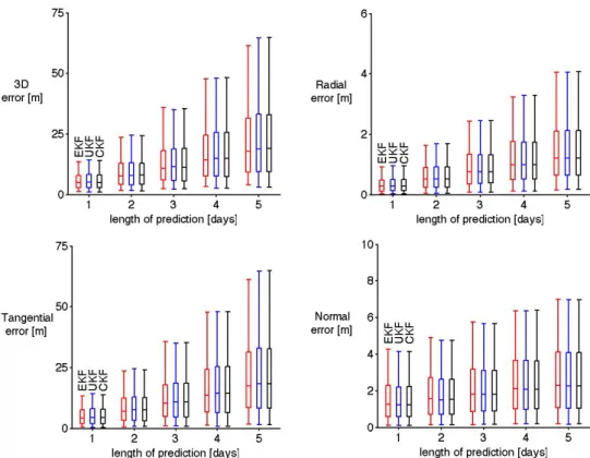
This topic is explored in publication [PI] and relates to the problem of estimating the initial state of a GNSS satellite using previously received ephemeris data and predicting the state into the future. This has practical applications e.g. in reducing the time required for first positiong fix in an autonomous GNSS positioning device. The problem is formulated as a Gaussian filtering problem with unknown process noise variance. Major part of the problem is estimating the unknown process noise, that has a significant impact especially to the estimated variance of the predicted orbit. Consistent estimates of the variance are important for assessing the reliability of the prediction results. Finally, the prediction results using the extended Kalman filter are compared to more sophisticated sigma-point based filters.
Developing online algorithms for statistical inference in regression and filtering problems with robust measurement noise models
These algorithms are especially important in applications where the problem needs to be solved in real time with possibly limited computational resources (e.g. online positioning in a mobile phone). Typically a Gaussian noise assumption is used to enable efficient Kalman filter based algorithms for state estimation. Measurement outliers, often encountered in real datasets, however do not fit into the Gaussian assumption and can distort the results.
Publication [PII] presents a variational Bayes based algorithm for linear regression problems with Gaussian scale mixture measurement noise distribution. Special cases from the Gaussian scale mixture family of distributions include the multivariate
t-distribution, the multivariate Laplace distribution and the contaminated normal
distribution.
Section 3.3 extends the regression results to the nonlinear filtering problem and presents a variational Bayes based outlier robust filtering algorithm for Laplace and contaminated normal measurement noise models. This extends the results presented in [1] and [44] which consider outlier robust filtering based on the multivariate t
distribution.
Improving Gaussian filtering based smoothing for continuous-discrete Gaussian models using iterative variational Gaussian algorithm
These results apply for continuous-discrete models, where the transition process is modelled with a continuous stochastic differential equation (SDE) and measurements are taken at discrete time instants. These kind of systems can be found for example in navigation, systems biology and weather forecasting [13, 32, 59]. Computing the exact smoothing solution requires solving the partial differential equations related to the process SDE [27]. The exact solution is tractable only for some special cases and approximations must be used.
In publication [PIII] an iterative variational Bayes based smoothing algorithm is presented for approximating the posterior distribution. The presented variational Gaussian smoothing algorithm extends the results in [10 – 12] by allowing a more general stochastic process with possibly singular diffusion matrix for describing the system dynamics. Furthermore, a practical algorithm is presented based on the Gaussian filtering based smoothing results in [51]. The presented algorithms use the Gaussian filtering based smoothing results as initial conditions and approximate the
1.2. Research objectives and scope of the research 5
intractable Gaussian integrals with linearisation or sigma-point based methods. It is shown how for some highly nonlinear systems, the variational Gaussian smoother can be used to iteratively improve the Gaussian filtering based smoothing results.
Improving the efficiency of particle Markov chain Monte Carlo methods using twisted particle filters and Gaussian filtering methodology
Particle Markov chain Monte Carlo (PMCMC) methods for model parameter estimation (system identification) use particle filters at each iteration of a MCMC sampler to estimate the marginal likelihood and generate samples from the posterior distribution [5]. The advantage of these methods is that they target the true posterior probability distribution. However, running a particle filter at each iteration means that they are often computationally heavy.
Publication [PIV] shows how the efficiency of the PMCMC algorithm can be improved using twisted particle filters. The twisted particle filter builds upon standard particle filters by adding a special weighting to the sampling law, and can be used to optimally estimate the marginal likelihood of the state-space model [58]. This thesis presents a generalization of the twisted particle that allows a variety of different resampling schemes. Also, a practical implementation of the twisted particle filter is presented for Gaussian models based on the Gaussian filtering methodology. An example with real data shows how the twisted particle filter can deliver computational gains in the particle Markov chain Monte Carlo algorithm compared to standard particle filters.
2 Model description
2.1
Discrete-time state-space model
A general probabilistic discrete time state-space model can be presented in a form
x0∼p(x0), xk ∼p(xk|xk−1), k≥1 (2.1a)
yk ∼p(yk|xk), k≥0, (2.1b)
where xk ∈ Rn is the state at time tk, yk ∈ Rm is the measurement at time
tk, p(x0) is the initial distribution, p(xk|xk−1) is the distribution for the state transition process, also called dynamic model, and p(yk|xk) is the distribution for the measurement process, also called measurement model.
The system is assumed to be Markovian i.e. the state sequence{xk}is a Markov sequence and the measurement yk given statexk is conditionally independent of the state and measurement histories:
p(xk|x0:k−1,y0:k−1) =p(xk|xk−1), k≥1, (2.2a)
p(yk|x0:k,y0:k−1) =p(yk|xk), k≥0. (2.2b) With these assumptions satisfied, the joint density of the model can be presented by
p(x0:k,y0:k) =p(x0)p(y0|x0) k Y
s=1
p(ys|xs)p(xs|xs−1), k≥0. (2.3)
The following subsections describe the specific state-space models that are considered in this thesis.
2.2
Gaussian model
Gaussian state-space model can be presented in the form
x0∼N(m−0,P −
0), xk∼N(fk−1(xk−1),Qk−1), k≥1, (2.4a)
yk∼N(hk(xk),Rk), k≥0, (2.4b)
where N(m,P) denotes a multivariate Gaussian distribution with mean vectormand
covariance matrix P. The transition functions fk−1: Rn →Rn and measurement functions hk:Rn →Rm can be any (nonlinear) functions of the state.
An alternative presentation for (2.4), which emphasizes the additive nature of the noise processes, is given by
x0∼N(m0,P0), xk =fk−1(xk−1) +wk−1, k≥1, (2.5a)
yk =hk(xk) +vk, k≥0, (2.5b)
where{wk}and{vk}are zero-mean Gaussian white noise sequences, with covariance matricesE[wkwTs] = Qkδks andE[vkvTs] = Rkδks respectively. In order to satisfy the Markov assumptions (2.2), the random variablesx0,{wk}and{vk}are assumed mutually independent.
If the functionsfk−1 andhk are linear, the model is called a linear Gaussian model. The linear Gaussian model is an important special case, since it is one of the only special cases that allows an exact solution of the state inference problem.
2.2.1
Models with outlier robust measurement distribution
Real datasets sometimes contain outliers, or extreme observations, that do not fit into the Gaussian assumption about the measurement distribution. Under the Gaussian assumption, even a single outlier can have a significant effect on the results of the statistical inference (see e.g. [24, p. 435]). Outlier-robust inference can be achieved using a measurement distribution with heavier tails than the Gaussian distribution. Here heavy-tailed means distributions that give relatively high probability also for observations far away from the mean.
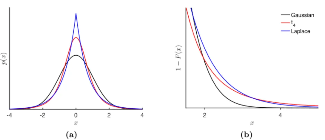
Fig. 2.1 shows the probability densities and the heavy-tailedness property of two often used outlier robust measurement distributions: the (Student’s)t distribution,
with degrees of freedom 4, and the Laplace, or double exponential, distribution. Compared to the Gaussian distribution with the same mean and variance, thetand
2.2. Gaussian model 9 -4 -2 0 2 4 (a) 2 4 Gaussian t4 Laplace (b)
Figure 2.1: Probability density functions (a) and right tail probabilities (b) for Gaussian, tand Laplace distributions with the same mean and variance.
Laplace distributions have more probability mass in the tails of the distribution, and therefore observations far away from the mean are not so rare.
An outlier robust version of the Gaussian model (2.4) is obtained by using a
t, Laplace or some other heavy-tailed distribution for the measurement model
(2.4b). For computational purposes (see Section 3.3) it is convenient to define the outlier-robust measurement distribution using the hierarchical model
yk∼N(hk(xk),Rk/uk), uk ∼p(uk), k≥0, (2.6) where {uk > 0} is a sequence of independent auxiliary random variables, and the distribution p(uk) controls the form of the distribution for the measurements. The measurement distribution obtained using (2.6) is also called a Gaussian scale mixture distribution [2], sincep(yk|xk) is given by
p(yk|xk) = Z
RN(
yk|hk(xk),Rk/uk)p(uk) duk. (2.7)
The following list shows how to choosep(uk) to obtain three common outlier-robust measurement distributions: the multivariatet, multivariate Laplace and multivariate
contaminated normal distributions [PII]:
• The multivariatetdistribution[36], with degrees of freedomν, is obtained
by choosing [39] p(uk)∝u ν 2−1 k e −ν 2uk. (2.8)
The density (2.7) is given by p(yk|xk)∝ 1 + 1 ν(yk−hk(xk)) TR−1 k (yk−hk(xk)) −ν+2m . (2.9)
• The multivariate Laplace distribution[37, p. 296] is obtained by choosing p(uk)∝u−k2e
−u−1k . (2.10)
The density (2.7) is given by
p(yk|xk)∝ Km/2−1 q 2(yk−hk(xk))TRk−1(yk−hk(xk)) q 1 2(yk−hk(xk)) TR−1 k (yk−hk(xk)) m/2−1 , (2.11)
whereKp is a modified Bessel function of the second kind with orderp. • The multivariate contaminated normal distribution[39] is obtained
by choosing
p(uk) = (1−)δ(uk−1) +δ(uk−1/c), (2.12) where 0< <1 andc >1. The density (2.7) is given by
p(yk|xk) = (1−)N(yk|hk(xk),Rk) +N(yk|hk(xk), cRk), (2.13) wheregives the probability of obtaining an outlier andcis a variance scaling
factor for the outlier observations. The distribution (2.13) is a multivariate generalization of the contaminated normal distribution introduced in [54]. More general Gaussian scale mixture measurement distributions can be obtained by taking the auxiliary variable’s distributionp(uk) from the Gamma or inverse-Gamma families [PII].
2.3
Continuous-discrete Gaussian state-space model
Many real dynamical systems are most easily described in continuous time i.e. using differential equations based on physical principles or empirical models. However, the measurements are nowadays often collected at discrete time instants e.g. using digital sensors or sampling from an analog sensor.
2.4. Example: target tracking 11
The continuous-discrete Gaussian state-space model is described by
x(t0)∼N(m0,P0), x˙ =f(x, t) + L(t)w(t), t≥t0, (2.14a) yk∼N(hk(x(tk)),Rk), k≥0, (2.14b) wheref:Rn+1→Rn is the transition function,w(t)∈Rd is a zero-mean Gaussian white noise stochastic process with covariance functionE[w(t)wT(τ)] = Q(t)δ(t−τ) and L: R→Rn×d. The measurement model is the same as in the discrete-time Gaussian state-space model.
Note that the white noise process is by definition discontinuous everywhere and therefore the differential equation in (2.14a) is not analysable by standard calculus rules. Mathematically rigorous treatment of the continuous-discrete model requires theory of stochastic differential equations and stochastic calculus (see e.g. [27, 43]). However, the presentation (2.14a) is still intuitively useful as a continuous-time version of the discrete-time Gaussian model (2.5a).
The continuous-time model (2.14a) can in theory be converted to the equivalent discrete-time model by solving the integral equation
x(tk) =x(tk−1) + Z tk tk−1 f(x(t), t) dt+ Z tk tk−1 L(t)w(t) dt, (2.15)
where the latter integral is interpreted as a stochastic Itô integral (see e.g. [27]). For the linear case, withf(x, t) = F(t)x, solving (2.15) gives [27, pp. 199-200]
x(tk) = Φ(tk, tk−1)x(tk−1) +wk−1, (2.16) where the state-transition matrix Φ(tk, tk−1) is the solution, at timet=tk, of the matrix differential equation
d
dtΦ(t, tk−1) = F(t)Φ(t, tk−1), Φ(tk−1, tk−1) = I, (2.17)
and{wk}is a zero-mean Gaussian white noise sequence with covariance matrix E[wkwsT] = Z tk+1 tk Φ(tk+1, τ)L(τ)Q(τ)LT(τ)ΦT(tk+1, τ) dτ δks. (2.18)
2.4
Example: target tracking
Throughout this introduction, the following example is used to demonstrate the presented methods. The example is motivated by a target tracking problem, where
the goal is to estimate the trajectory of some physical object e.g. a vehicle or a person. The state of the object is given by a vectorxT(t) = [rT(t),vT(t)], where r(t)∈R2 andv(t)∈R2 are the position and velocity of the target in Cartesian coordinates at timet≥0. A typical model for the state transition process is the
constant velocity model given formally by [13, p. 269] ¨
r(t) =w(t), (2.19)
where w(t) ∈ R2 is a zero-mean Gaussian white noise stochastic process with covariance given by
E[w(t)wT(τ)] =q2I2×2δ(t−τ), (2.20) whereq >0.
The continuous-time transition model is given by " ˙ r(t) ˙ v(t) # = " 02×2 I2×2 02×2 02×2 # | {z } F(t) " r(t) v(t) # + " 02×2 I2×2 # | {z } L(t) w(t). (2.21)
The state transition model is linear, so the continuous-time model can be exactly discretized using (2.16)-(2.18) giving (see also [13, p. 270])
xk= Fkxk−1+wk−1, (2.22) where Fk = " I2×2 I2×2∆tk 02×2 I2×2 # , (2.23)
∆tk =tk−tk−1 and{wk}k≥0is a zero-mean Gaussian white noise sequence with covariance E[wkwTs] =q 2 " (∆tk)3 3 I2×2 (∆tk)2 2 I2×2 (∆tk)2 2 I2×2 ∆tkI2×2 # δks. (2.24)
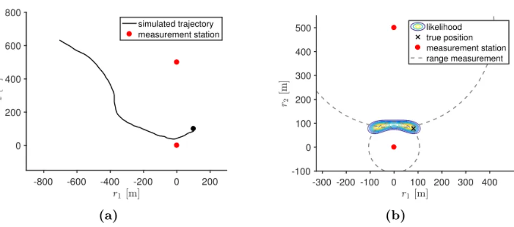
The measurements come from two stationary rangefinders (measurement stations) located at coordinates s1 = [0,0]T and s2 = [0,500]T. The measurements are modeled by yk =h(r(tk),v(tk)) +zk, (2.25) where h(r,v) = " kr−s1k kr−s2k # , (2.26)
2.4. Example: target tracking 13 -800 -600 -400 -200 0 200 0 200 400 600 800 simulated trajectory measurement station (a) -300 -200 -100 0 100 200 300 400 -100 0 100 200 300 400 500 likelihood true position measurement station range measurement (b)
Figure 2.2: (a) Simulated route and (b) the likelihood at one time instant.
and{zk}k≥1is a zero-mean Gaussian white noise sequence with covarianceE[zkzTs] =
σ2I
2×2δks, σ2 > 0. Fig. (2.2) shows a simulated route and the likelihood for a single measurement. Since the measurements do not depend on the velocityv, the
likelihood can be plotted by computingp(yk|r(tk)) on a dense grid forr1 andr2. Typically for two range measurements, the likelihood is bimodal, and the modes are located at the intersections of the ring shaped likelihoods of the individual ranges.
3 Methods for sequential Bayesian
inference
3.1
Bayesian inference in discrete-time state-space models
Given measurements y0:t, the full solution to the discrete-time state inference problem for the model in Eq. (2.1) is given by the Bayes theorem
p(x0:t|y0:t) =
p(y0:t|x0:t)p(x0:t)
p(y0:t)
, (3.1)
wherep(y0:t|x0:t) is the likelihood,p(x0:t) is the prior andp(y0:t) is a normalization constant, also called marginal likelihood or evidence. Usually, instead of the full posterior distribution, we are interested in specific marginal posterior distributions of the state:
Filtering distribution p(xk|y0:k) gives the posterior distribution of the state at timekgiven all the measurements up to that time.
Smoothing distribution p(xk|y0:t) gives the posterior distribution of the state at time 0≤k≤tgiven all the available measurements.
The filtering distribution can be computed recursively, starting from the priorp(x0), using the Bayesian filtering equations
p(xk|y1:k−1) = Z
Rn
p(xk|xk−1)p(xk−1|y1:k−1) dxk−1, k≥1, (3.2a)
p(xk|y0:k)∝p(xk|y0:k−1)p(yk|xk), k≥0. (3.2b) The first equation (3.2a) is often called the prediction step and (3.2b) the update step.
The smoothing distribution can be computed using the backward-time recursion, started from the filtering distributionp(xt|y0:t) at timet, using [34]
p(xk|y0:t) =p(xk|y0:k) Z Rn p(xk+1|xk)p(xk+1|y0:t) p(xk+1|y0:k) d xk+1, t−1≥k≥0. (3.3) The smoothing presented by (3.3) is also called forward-backward smoothing, since it is based on first computing the forward-time filtering equations and then using the filtering distribution to compute the backward-time smoothing equations. An alternative formulation is the two-filter smoother [18, 23, 35].
In general the integrals in the filtering and smoothing equations are intractable and must be approximated. A special case is the linear Gaussian model, which allows an exact solution that can be computed using the Kalman filter and smoother algorithms. The approximation methods for the non-linear non-Gaussian case can be broadly divided into two classes, deterministic and stochastic approximations. The deterministic approximations replace the posterior distribution with a distribution that allows computationally tractable solution for the filtering and smoothing equations. Typically these are computationally light, but do not give any guarantee about the quality of the approximation. Examples are the Gaussian and factorized variational Bayes approximations.
The stochastic approximation methods are based on generating random samples from the posterior distribution; the samples can be used to approximate the posterior distribution and related expectations with arbitrary accuracy. These methods are however computationally intensive, which limits their use in large-scale or online inference problems. An example is the particle filter based on sequential Monte Carlo sampling.
3.2
Gaussian filtering and smoothing
Gaussian filtering and smoothing is a general framework for solving the Bayesian inference problem in Gaussian state-space models. It is based on approximating the non-Gaussian filtering and smoothing distributions with a Gaussian distribution [26, 49, 50, 60].
3.2. Gaussian filtering and smoothing 17
3.2.1
Gaussian filter
Assume that we have obtained the Gaussian approximation for the filtering distri-bution at time tk−1, given byp(xk−1|y0:k−1)≈N(xk−1|mk−1,Pk−1). Using the Gaussian moment matching [49, pp. 96-97], the prediction step (3.2a) is then given by p(xk|y0:k−1)≈N(xk|m−k,P−k), (3.4) where m−k = Z Rn fk−1(xk−1)N(xk−1|mk−1,Pk−1) dxk−1, (3.5a) P− k = Z Rn (fk−1(xk−1)−m−k)(fk−1(xk−1)−m−k)TN(xk−1|mk−1,Pk−1) dxk−1 + Qk−1. (3.5b)
Similarly, using the Gaussian approximation (3.4) and the Gaussian moment match-ing, the update step (3.2b) is given by
p(xk|y0:k)≈N(xk|mk,Pk), (3.6) where µk= Z Rn hk(xk)N(xk|m−k,P − k) dxk, (3.7a) Sk= Z Rn( hk(xk)−µk)(hk(xk)−µk) TN(x k|m−k,P − k) dxk+ Rk, (3.7b) Ck= Z Rn (xk−m−k)(hk(xk)−µk) TN(x k|m−k,P − k) dxk, (3.7c) Kk= CkS−k1, (3.7d) mk=m−k + Kk(yk−µk), (3.7e) Pk= P−k −KkSkKTk. (3.7f)
The recursion is started with the update step for the prior meanm−0 and variance
P−
0. If there is no measurement at k = 0, then the update step is left out and m0=m−0 and P0= P−0.
The resulting Gaussian filter is summarized in Algorithm 1. Figure 3.1 illustrates one step of the Gaussian filter. As can be seen, the Gaussian approximation cannot capture the true shape of the resulting posterior distribution, but is often sufficiently accurate in practical applications.
Algorithm 1Gaussian filter
1: Setm0and P0using (3.7)
2: fork= 1 totdo
3: Setm−k and P−k using (3.5)
4: Setmk and Pk using (3.7)
5: end for
If the transition and measurement functions are linear, the Gaussian filter reduces to the Kalman filter [31]. For non-linear transition and measurement functions, the general Gaussian filter is intractable, since the Gaussian integrals in (3.5) and (3.7) cannot be computed explicitly. Many of the common non-linear filters can be seen as special cases of the Gaussian filter when the Gaussian integrals are approximated with a specific numerical integration method. Using first order Taylor series linearization for the transition and measurement functions gives the extended Kalman filter (EKF). Using the cubature or the Gauss-Hermite integration rule to approximate the Gaussian integrals give the cubature Kalman filter (CKF) [6, 60] and Gauss-Hermite Kalman filter (GHKF) [8, 26] respectively. The unscented Kalman filter (UKF) [28, 29, 57] can be also seen as a Gaussian filtering algorithm by a generalization of the CKF integration rule [49, p. 108].
3.2.2
Gaussian smoother
The general Gaussian fixed-interval smoother can be derived in a similar way as the Gaussian filter by assuming thatp(xk+1|y0:t)≈N(xk+1|msk+1,Psk+1), and then using the Gaussian moment matching to get the approximation [50], [49, p. 152]
p(xk|y0:t)≈N(xk|msk,P s k), (3.8) where Dk+1= Z Rn( xk−mk)(fk(xk)−m−k+1) TN( xk|mk,Pk) dxk (3.9a) Gk= Dk+1(P−k+1) −1 (3.9b) msk=mk+ Gk(msk+1−m − k+1) (3.9c) Ps k= Pk+ Gk(Psk+1−P−k+1)G T k. (3.9d)
The resulting Gaussian smoother is summarized in Algorithm 2. Note that the matri-ces Dk+1and Gk depend only on filtering results and can therefore be precomputed and stored during the filtering recursion.
3.2. Gaussian filtering and smoothing 19
(a) (b)
(c) (d)
Figure 3.1: Contour lines for the prior distribution (a), prediction distribution (b),
measurement likelihood (c) and posterior distribution (d) for the first filtering step of the tracking example. Solid black line in figures (c) and (d) shows contours of the Gaussian approximation computed with EKF.
For a linear model, the Gaussian smoother reduces to the Rauch-Tung-Striebel smoother (RTSS) introduced in [46]. The extended RTSS [20] is obtained by using the first order Taylor series approximation for the transition and measurement functions. The unscented RTSS [48], cubature RTSS [7] and Gauss-Hermite RTSS [50], [49, p. 153-154] can be obtained by using the unscented, cubature and Gauss-Hermite integration rules for the Gaussian integral in (3.9).
Algorithm 2Gaussian smoother
1: Setmst←mtand Pst ←Pt
2: fork=t−1 to 0 do
3: Setm−k+1 and P−k+1 using (3.5)
4: Setmsk and Psk using (3.9)
5: end for
3.2.3
Numerical approximations for the Gaussian integrals
This section provides a brief overview of the Taylor series linearization and sigma-point based numerical approximation methods for the Gaussian integrals in (3.5), (3.7) and (3.9). Detailed discussion of the presented methods can be found e.g. from [49].
Taylor series linearization
The EKF and extended RTSS can be obtained by linearizingfk−1 andhk using the first order Taylor series expansion given by
fk−1(xk−1)≈fk−1(mk−1) + Fk−1(xk−1−mk−1), (3.10a)
hk(xk)≈hk(mk−) + Hk(xk−m−k), (3.10b) where Fk−1∈Rn×n is the Jacobian matrix offk−1evaluated at mk−1, and Hk∈ Rm×n is the Jacobian matrix ofh
k evaluated atm−k given below. Using (3.10a), the prediction step (3.5) is given by
m−k =fk−1(mk−1) (3.11a)
P−
k = Fk−1Pk−1F T
k−1+ Qk−1. (3.11b)
Using (3.10b), the variables µk, Sk and Ck in the update step (3.7) are given by
µk=hk(m−k) (3.12a)
Sk= HkP−kH T
k + Rk (3.12b)
Ck= P−kHTk. (3.12c)
And the matrix Dk+1 in the smoothing step (3.9) is given by
Dk+1= PkFTk. (3.13)
3.2. Gaussian filtering and smoothing 21
The sigma-point approximation is based on approximating the Gaussian integral on a deterministically chosen grid. For a nonlinear function g, the Gaussian integral is
approximated using Z
g(x)N(x|m,P) dx≈X
i∈I
wig(Xi), (3.14)
where the index setI, sigma-points{Xi}i∈I and related weights{wi}i∈I depend on the chosen sigma-point rule. The sigma-points are typically chosen based on the mean and variance of the Gaussian distribution and are given by
Xi=m+√Pξi, i∈I, (3.15)
where the matrix square-root is defined here with P =√P√PT and the vectorsξi
depend on the chosen sigma-point rule. Different rules for choosing the sigma-points and weights include e.g. the cubature, unscented and Gauss-Hermite integration rules [49].
The prediction step of the sigma-point filter is given by
Xik−1=mk−1+ p Pk−1ξi, i∈I, (3.16a) m−k =X i∈I wifk−1(Xik−1), (3.16b) P− k = X i∈I wi(fk−1(Xik−1)−m − k)(fk−1(Xik−1)−m − k) T + Q k−1. (3.16c) The variablesµk, Sk and Ck in the update step (3.7) are given by
ˆ Xik =m−k + q P− kξ i , i∈I, (3.17a) µk =X i∈I wihk( ˆX i k), (3.17b) Sk = X i∈I wi(hk( ˆX i k)−µk)(hk( ˆX i k)−µk) T + R k, (3.17c) Ck = X i∈I wi( ˆXik−m−k)(hk( ˆX i k)−µk)T. (3.17d)
The matrix Dk+1 in the smoothing step (3.9) is given by Xi k=mk+ p Pkξi, i∈I, (3.18a) Dk+1= X i∈I wi(Xik−mk)(fk(Xik)−m−k+1) T. (3.18b)
3.3
Outlier-robust Gaussian filtering
In [PII] outlier robust inference is presented for the multivariate regression problem. The regression model can be seen as a special case of a state-space model with the identity function as the transition function, and to better tie the results to the topic of the thesis, this section extends the regression results to the dynamic state-space model case.
Outlier robust filtering and smoothing using the multivariate t distribution is
presented in [1, 44]. The results for the robust multivariate regression in [PII] can be combined with the recursive algorithm in [44] to obtain a general recursive outlier-robust filtering and smoothing equations, having the multivariatet, multivariate
Laplace and contaminated normal distributions as special cases. For simplicity, the introductory part only deals with the three special cases that are the most useful in practical applications.
The state-space model is given by (2.4a) and (2.6), and the filtering distribution at timek is given by
p(xk|y0:k) = Z
Rp(xk, uk|y0:k) duk. (3.19)
Computing (3.19) is intractable, and approximate methods must be used.
The variational Bayes (VB) method is a general framework for forming approximate distributions using variational calculus. Usually the VB method refers to finding factorized approximations that minimize the Kullback-Leibler (KL) divergence of the approximation with respect to the original distribution [15, 17, 42].
Applying the VB method for the filtering problem results in a factorized approxi-mation of the form
p(xk, uk|y1:k)≈q(xk)q(uk), (3.20) where the distributionsq(xk) andq(uk) are chosen to minimize the KL divergence [38] given by KL [q(xk)q(uk)||p(xk, uk|y0:k)] = Z R Z Rn q(xk)q(uk) log q(xk)q(uk) p(xk, uk|y0:k) dxkduk. (3.21) Note that combining (3.19) and (3.20) gives p(xk|y0:k)≈q(xk).
3.3. Outlier-robust Gaussian filtering 23
It can be shown that the optimal distributionsq(xk) andq(uk) minimizing (3.21) satisfy [17, pp. 465-466]
logq(xk) = Z
Rlogp(xk, uk,y0:k)q(uk) duk+ const, (3.22a)
logq(uk) = Z
Rnlog
p(xk, uk,y0:k)q(xk) dxk+ const. (3.22b) The equations (3.22) do not give an explicit solution, but can be used as the basis for an iterative coordinate-descent algorithm that converges to the minimum [17, p. 466].
The functional forms forq(xk) andq(uk) are found by computing the integrals in (3.22a) and (3.22b). For (3.22a) we have [44]
logq(xk) =−¯ uk 2 (yk−hk(xk))TRk−1(yk−hk(xk)) −1 2(xk−m−k) T(P− k) −1(x k−m−k) + const, (3.23) where ¯ uk= Z Rukq(uk) duk. (3.24)
For non-linear measurement function hx(xk) (3.23) does not correspond to any standard distribution, but since it is of the same form as the distribution in the update step of the Gaussian filter, we can use the Gaussian approximation
q(xk)≈N(xk|mk,Pk), where the meanmk and covariance Pk are computed using
µk = Z Rn h(xk)N(xk|m−k,P − k) dxk, (3.25a) Sk = Z Rn( h(xk)−µk)(h(xk)−µk)TN(xk|m−k,P − k) dxk+ 1 ¯ ukR k, (3.25b) Ck = Z Rn( xk−m−k)(h(xk)−µk)TN(xk|mk−,P − k) dxk (3.25c) Kk = CkS−k1 (3.25d) mk =m−k + Kk(yk−µk) (3.25e) Pk = P−k −KkSkKTk. (3.25f) For (3.22b) we have logq(uk) =− ¯ γk 2 uk+ m 2 loguk+ logp(uk), (3.26)
where ¯ γk= trace Z Rn( yk−h(xk))(yk−h(xk))Tq(xk) dxk R−1 k (3.27) For the three different p(uk), given in (2.8), (2.10) and (2.12), and corresponding to multivariatet, Laplace and contaminated normal distributions, the distribution q(uk) in (3.26) is given by the following formulas [PII]
• Multivariatet distribution, withν degrees of freedom: q(uk) is a Gamma distribution with density
q(uk)∝u (ν+m)/2−1 k e −uk(ν+¯γk)/2 (3.28) and mean ¯ uk= ν+m ν+ ¯γk . (3.29)
• multivariate Laplace distribution: q(uk) is a generalized inverse Gaussian distribution with density
q(uk)∝u m/2−2 k e −1 2(¯γkuk+2u−1k ), (3.30) and mean ¯ uk= r 2 ¯ γk Km/2( √ 2¯γk) Km/2−1( √ 2¯γk) , (3.31)
whereKp is a modified Bessel function of the second kind with orderp. • multivariate contaminated normal distribution: q(uk) is a two-component
mixture with density1
q(uk)∝(1−)e− ¯ γk 2 δ(uk−1) +c−1e− ¯ γk 2cδ(uk−1/c), (3.32) and mean ¯ uk =(1 −)e−¯γk/2+c−2e−¯γk/(2c) (1−)e−¯γk/2+c−1e−¯γk/(2c). (3.33) The resulting outlier robust VB filter is summarized in Algorithm 3. Here the parameternmaxdetermines the number of iterations in the VB update step. Instead of a fixed number of iterations, the termination condition could be obtained by monitoring the variational lower bound [PII]. However, computing the variational lower bound increases the computational cost for each iteration and in practice it is often sufficient to use a fixed number of iterations.
3.4. Particle filtering 25
Algorithm 3outlier-robust VB filter
1: fori= 1 tonmax do
2: Setm0 and P0 using (3.25)
3: Σ0← R (y0−h0(x0))(y0−h0(x0))TN(x0|m−0,P − 0) dx0 4: γ¯0←trace(Σ0R−01)
5: Set ¯uk using (3.29) for multivariatet, (3.31) for multivariate Laplace, (3.33) for multivariate contaminated normal
6: end for 7: fork= 1 totdo 8: mk−←R fk−1(xk−1)N(xk−1|mk−1,Pk−1) dxk 9: P−k ←R(fk−1(xk−1)−m−k)(fk−1(xk−1)−m−k) TN(x k−1|mk−1,Pk−1) dxk+ Qk−1 10: u¯k←1 11: fori= 1 tonmax do
12: Setmk and Pk using (3.25)
13: Σk ←R(yk−hk(xk))(yk−hk(xk))TN(xk|mk,Pk) dxk
14: ¯γk ←trace(ΣkRk−1)
15: Set ¯uk using (3.29) for multivariatet, (3.31) for multivariate Laplace, (3.33) for multivariate contaminated normal
16: end for
17: end for
3.4
Particle filtering
The particle filter, or sequential Monte Carlo method, uses sequential importance sampling to draw samples from the filtering distribution. The set of samples, or particles, can then be used to approximate the filtering distribution and related expectations. The particle filter can be used for the general state-space model (2.1). Let{xi
k∈Rdx}ni=1denote the set of particles and{wik∈[0,1]}ni=1the set of related weights at timek. The weights satisfyPn
i=1w i
k = 1. The approximation for the
filtering distribution is given by
p(xk|y0:k)≈ N X i=1 wikδ(xk−xik). (3.34) The particlesxi
k are drawn from an importance distributionq(xk|xik−1,y0:k) and the weights are evaluated using
wik∝wik−1p(yk|x i k)p(xik|xik−1) q(xi k|xik−1,y0:k) . (3.35)
To avoid problems with degeneracy, the particle filters use a resampling step to discard particles with small weights and duplicate particles with large weights [47].
The particle filter algorithm is presented in Algorithm 4. Here resampling is done at stepiif the effective sample size, given by
Neff= N X i=1 1 (wi k)2 , (3.36)
goes below a predefined thresholdNthr.
Using Equation (3.34) the expectations with respect to the filtering distribution can be approximated using
E[g(xk)|y0:k]≈ N X
i=1
wkig(xik). (3.37)
As the number of particles increases, this approximation approaches the true value of the expectation by the law of large numbers [19].
Taking the transition distribution as the importance distribution, i.e.q(xk|xk−1,y0:k) =f(xk|xk−1), gives the bootstrap particle filter [25]. The bootstrap particle filter is simple to implement, but can be inefficient since the particles are propagated without using any measurement information. An optimal importance distribution, in the sense of minimizing the variance of the weights in a single time step, can be shown to be q(xk|xk−1,y0:k)∝p(yk|xk)p(xk|xk−1) [21]. For nonlinear and non-Gaussian measurement models the optimal importance distribution is often intractable, but can be approximated e.g. using Kalman filter extensions [21, 55]. The auxiliary particle filter [45] uses the measurement information in the resampling step and effectively mimics the use of the optimal importance distribution.
3.5
Filtering and smoothing in continuous-discrete models
For the continuous-discrete model, the statex(t) is now continuous in time.
There-fore the filtering distribution using measurements up to timek is defined for the
whole time interval [tk, tk+1) and denoted by
p(x(t)|y0:k), tk ≤t < tk+1. (3.38) Similarly, the smoothing distribution is defined for time interval [t0, tt] and denoted by
p(x(t)|y0:t), t0≤t≤tt. (3.39)
For a fully continuous (i.e. both dynamics and measurements are continuous in time) linear Gaussian model, the solution to the filtering problem is given by the
3.5. Filtering and smoothing in continuous-discrete models 27
Algorithm 4Particle filter
1: Samplexi0∼p0(x0) and setw0i ←p(y0|xi0) for 1≤i≤N
2: for1≤k≤t do 3: for1≤i≤N do 4: Samplexik∼q(xk|xik−1) 5: Setwi k←wki−1 p(yk|xik)p(xik|xik−1) q(xi k|x i k−1) 6: end for 7: SetNeff←P N i=1 1 (wi k)2 8: if Neff< Nthr then 9: Set (xi k) N i=1←resample((xik) N i=1,(wki) N i=1) 10: Setwi k←1/N for alli 11: end if 12: end for
Kalman-Bucy filter [30]. The continuous-discrete Kalman filter is a combination of the continuous-time Kalman-Bucy filter and the discrete-time Kalman filter, where the Kalman-Bucy prediction equations are used between observations and the Kalman filter update step at observation times [27]. The continuous-time Rauch-Tung-Striebel smoother [46] uses the filtering solution and gives a recursive solution for the smoothing problem in the linear continuous-discrete system.
3.5.1
Gaussian filtering and smoothing for the
continuous-discrete model
For non-linear models, the filtering and smoothing distributions are no longer Gaussian, but similarly to the discrete-time case, we can consider Gaussian approx-imations for these densities. This means approximating the filtering and smoothing densities with
p(x(t)|y0:k)≈N(x(t)|m(t),P(t)), tk ≤t < tk+1,0≤k≤t, (3.40a)
p(x(t)|y0:k)≈N(x(t)|ms(t),Ps(t)), t0≤t≤tt, (3.40b) wheremk(t) andms(t) are the mean functions and P(t) and Ps(t) are the auto-covariance functions for the approximating Gaussian distributions. The filtering and smoothing problem now reduces to finding the expressions for the mean and covariance functions.
In this thesis, two methods for computing the Gaussian approximations are presented. The classical Gaussian approximation is based on recursions similar to the
discrete-time case, and gives approximate solutions for the mean and covariance functions in the filtering and smoothing problem [51]. Another solution is based on the variational Bayes methodology, where the mean and covariance functions for the smoothing solution are chosen to minimize the KL-divergence between the true and approximate solutions [11, 12]. In some sense, this can be seen as an iterative way to improve the classical Gaussian approximation [PIII].
3.5.2
Gaussian filtering based approximation
In the prediction step, the mean and covariance functions are propagated from time
tk−1to time tk by solving the differential equations ˙ m(t) = Z Rn f(x, t)N(x|m(t),P(t)) dx, (3.41a) ˙P(t) = Z Rn ( x−m(t))fT(x, t) +f(x, t)(x−m(t))TN( x|m(t),P(t)) dx+ Σ(t), (3.41b) with initial conditionsmk−1(tk−1) and P(tk−1) obtained from the previous step. In the update step, the information from the latest measurement yk is used to update the predicted estimates m(t−k) and P(t−k) using equations
µk=E[hk(x(t−k)), (3.42a) Sk=E (hk(x(t−k))−µk)(hk(x(t−k))−µk) T + Rk, (3.42b) Kk=E (x(t−k)−m(t−k))(hk(x(t−k))−µk) T S−1 k , (3.42c) m(tk) =m(t−k) + Kk(yk−µk), (3.42d) P(tk) = P(t−k)−KkSkKTk. (3.42e)
Gaussian approximation for the smoothing distribution can be derived using several different approaches. A numerically stable and computationally light solution is given by [51] ˙ ms(t) =E[f(x(t), t)] + E[f(x(t), t)(x(t)−m(t))T] + Σ(t)P−1(t)(ms(t)−m(t)), (3.43a) ˙Ps(t) = ( E[f(x(t), t)(x(t)−m(t))T] + Σ(t))P−1(t)Ps(t) + Ps(t)P−1(t)(E[f(x(t), t)(x(t)−m(t))T]T+ Σ(t))−Σ(t), (3.43b) where the expectations are with respect to the filtering distribution.
3.5. Filtering and smoothing in continuous-discrete models 29
If the Jacobian Fx(x, t) off(x, t) is available, we can use the result
E[f(x, t)(x−m)T] =E[Fx(x, t)]P (3.44)
in the filtering and smoothing equations. Since the expectations in the smoothing equations are with respect to the filtering density, they can be precomputed already during the filtering stage.
3.5.3
Variational Gaussian approximation
The variational Gaussian approximation, first presented in [11], for the continuous-discrete smoothing problem is based on approximating the intractable smoothing process with a linear stochastic differential equation
dx= [−A(t)x(t) +b(t)]dt+pΣ(t)dβ(t), (3.45)
where A(t) andb(t) are parameters of the approximation andβ(t)is a Brownian
stochastic process with identity diffusion matrix. The matrix Σ(t) is called the
effective diffusion matrix of the original stochastic differential equation in Eq. (2.14a) and is given by
Σ(t) = L(t)Q(t)LT(t). (3.46)
For simplicity, only the case of non-singular effective diffusion matrix is considered in this introduction. Derivation of the equations for some singular cases can be found in [PIII].
The solution to the linear stochastic differential equation (3.45) is a Gaussian process, with mean and variance defined by ordinary differential equations
˙
m(t) =−A(t)m(t) +b(t), (3.47a)
˙P(t) =−A(t)P(t)−P(t)AT(t