Timothy Peter Jackson
ORCID Identifier: 0000-0002-6142-8882
Submitted in total fulfillment of the requirements of
the degree of Doctor of Philosophy
Submitted September 2018; Revised December 2018
Economics Section
Cardiff University
ANNEX 1:
Specimen layout for Declaration/Statements page to be included in a thesis.
DECLARATION
This work has not been submitted in substance for any other degree or award at this or any other university or place of learning, nor is being submitted concurrently in candidature for any degree or other award.
Signed (Tim Jackson) Date 09/01/2019
STATEMENT 1
This thesis is being submitted in partial fulfillment of the requirements for the degree of PhD
Signed (Tim Jackson) Date 09/01/2019
STATEMENT 2
This thesis is the result of my own independent work/investigation, except where otherwise stated, and the thesis has not been edited by a third party beyond what is permitted by Cardiff University’s Policy on the Use of Third Party Editors by Research Degree Students. Other sources are acknowledged by explicit references. The views expressed are my own.
Signed (Tim Jackson) Date 09/01/2019
STATEMENT 3
I hereby give consent for my thesis, if accepted, to be available online in the University’s Open Access repository and for inter-library loan, and for the title and summary to be made available to outside organisations.
Signed (Tim Jackson) Date 09/01/2019
STATEMENT 4: PREVIOUSLY APPROVED BAR ON ACCESS
I hereby give consent for my thesis, if accepted, to be available online in the University’s Open Access repository and for inter-library loans after expiry of a bar on accesspreviously approved by the Academic Standards & Quality Committee.
Banks provide not one but two vital services. Bank deposits are the pre-ferred form of safe assets used for transactions, and bank loans allow busi-nesses to undertake risky endeavors. However, this creates a tension in bank business: deposit-holders require safety for bank liabilities to be liquid; while loan-holders want the freedom to take profitable business risks. A widely-used policy to guarantee the liquidity of bank deposits is the government provision of deposit insurance. This thesis considers some of the relative benefits and costs of deposit insurance relative to an alternative of ‘narrow banking’. This policy argues that a single bank liability structure cannot optimally provide both liquidity and credit. Instead, these two services should be provided by separate entities. These entities could share an owner, provided the safe ‘nar-row’ business can be credibly ring-fenced from the risky ‘wide’ bank. Narrow banks issue safe, short-term, debt which can be used for transactions and are invested solely in safe assets so as not to necessitate insurance. To pre-vent runs, we suggest that wide banks issue longer-term equity contracts to fund risky business credit. Savers are informed of risks up-front and updated through regular markings-to-market. This thesis considers the ability of a narrow banking system to provide liquidity and credit.
Acknowledgments
Throughout my PhD candidature at Cardiff University, I have received a tremendous amount of support and would like to devote a few paragraphs to expressing my gratitude to those who have contributed to my ability to submit today.
First and foremost, I would like to thank my co-authors Larry Kotlikoff and George Pennacchi who answered an email out-of-the-blue and have been extremely generous with their time in the past years. I have benefited tremen-dously from watching them work. I have also profited from collaborations and discussions with my supervisors Huw Dixon and Vo Phuong Mai Le, as well as Keqing Liu, Vito Polito, Mervyn King, Nobu Kiyotaki, Robert Townsend, Jeffrey Miron, John Cochrane, Tom Wilkening, Steven Williamson, Kevin Hoskin, Ian Woolford, David Delacr´etaz, Matthew Greenwood-Nimmo, An-drew Lilico, and Mike Wickens. Finally, I am grateful for the comments and criticism I received from my examiners Kent Matthews and Kevin Dowd. They have helped hone my ideas on this thesis and my future research.
I am grateful to all the professional staff in the business school, and in particular to Elsie Phillips, who have accompanied us throughout the past five years. Helen Walker has offered tremendous support as Director of the PhD programme and Melanie Jones as research panel convener.
It is hard to overstate the importance of the scholarships and travel funding I have received throughout my PhD candidature. Without the Economic and Social Research Council and Cardiff University, I would not have been able to conduct my Overseas International Visit to Boston University and other institutions in the United States to start the two papers that form the core of this thesis. I am also grateful to the Jim Perkins Traveling PhD Scholarship and everyone at the University of Melbourne who helped make a visit to the
Department so productive. The Money and Macro Finance Research Group also generously provided me a funded place on a workshop on Computational Methods from Jes´us Fern´andez-Villaverde hosted by the University of Oxford which has proved very useful in understanding what DYNARE does behind the scenes. I was also very fortunate to receive funding to visit the Reserve Bank of New Zealand, the only country in the OECD that does not have deposit insurance. I benefited greatly from discussions with practitioners on policy details and the important task of justifying policy to successive governments. My PhD colleagues have been essential to my candidature. Without Robert Forster and Lu´ıs Matos to share the ups and downs, and without Rachel Williams, James Wallace, Laura Reynolds, Emma Jones and Cassan-dra Bowkett, I am not sure I would have been able to complete.
Most importantly, I thank my girlfriend, Charlotte Cadman, for her con-stant support in the hardest years of the thesis. She continues to be the reason I can do something as ambitious as trying to get paid to think about things I find interesting. I am also grateful to both our families, particularly our parents – David and Wendy Jackson and Paul and Joanne Cadman – for their help throughout.
This thesis contains original research in Chapters 2 through 4. Chapter 2 is based on the following working paper:
Jackson, T., and Pennacchi, G.(2018): “How Should Governments Create Liquidity?” Working Paper.
Chapter 3 is based on the following working paper:
Jackson, T., and Kotlikoff, L. (2018) “Banks as Potentially Crooked Secret Keepers,” Working Paper.
Chapter 4 is based on the following working paper:
Dixon, H., and Jackson, T.(2018) “A Tale of Two Bailouts,” Work-ing Paper.
All co-authorship has taken place in accordance with the Graduate Re-search Training Policy of Cardiff University.
List of Figures ix
List of Tables xi
1 Introduction 1
We introduce and motivate the class of problems considered in this thesis and survey the relevant economics literature
2 How Should Governments Create Liquidity? 5
2.1 Introduction . . . 5
2.2 Liquidity Creation in a Fully-Private Banking System . . . 9
2.2.1 Tranching . . . 16
2.2.2 Quasi-Safe Asset Production . . . 20
2.3 Liquidity Creation with Government Deposit Insurance . . . 21
2.3.1 Taxes as a Source of Public Liquidity . . . 21
2.3.2 Deposit Insurance . . . 22
2.3.3 Cost Threshold for Effort under Deposit Insurance . . 28
2.3.4 The Maximum Level of Deposit Insurance . . . 29
2.3.5 Aggregate Liquidity under Deposit Insurance . . . 30
2.4 Liquidity Creation with Government Debt and Narrow Banking . . . 31
2.4.1 Equilibrium with Narrow Banks and Government
In-vestment . . . 33
2.4.2 Equilibrium with Narrow Banks and Government Rebate . . . 35
2.5 Numerical Illustrations . . . 37
2.5.1 Welfare Measures . . . 37
2.5.2 Calibration . . . 38
2.5.3 Comparative Statics . . . 41
2.6 Robustness of the Model’s Results . . . 44
2.7 Conclusions . . . 46
3 Banks as Potentially Crooked Secret-Keepers 48 3.1 Introduction . . . 49
3.2 Literature Review . . . 53
3.3 The Model . . . 58
3.4 Calibration . . . 61
3.5 Base Model Results. . . 62
3.6 Deposit Insurance . . . 72
3.7 Monitoring Banks . . . 75
3.7.1 Private Monitoring . . . 75
3.7.2 Information as a Public Good . . . 79
3.8 Regulation Through Disclosure . . . 81
3.9 Conclusion . . . 85
4 A Tale of Two Bailouts 87 4.1 Introduction . . . 88
4.2 Quantitative Easing . . . 90
4.2.1 US . . . 91
4.2.2 UK. . . 94
4.3 Bank Recapitalization and Nationalization . . . 104 4.3.1 USA . . . 104 4.3.2 UK. . . 109 4.3.3 Return on Investment . . . 111 4.4 Theoretical Model . . . 113 4.4.1 Model . . . 113 4.4.2 Results . . . 116 4.5 Conclusion . . . 120 5 Conclusion 122 A Appendices for Chapter 2 124 A.1 Proofs. . . 124
A.1.1 Proof of Lemma 1 . . . 124
A.1.2 Proof that high effort profits are decreasing in cost . . 126
A.1.3 Proof of Proposition 1 . . . 126
A.1.4 Proof of Lowest-cost bank leverage limit . . . 127
A.1.5 Proof of Proposition 3 . . . 127
A.2 Deposit insurance solution . . . 128
A.3 Welfare Measures . . . 130
B Appendices for Chapter 3 133 B.1 Deriving Sectoral Returns . . . 133
B.2 Solving for Allocation Decision with Private Monitoring. . . 134
List of Figures
2.1 Individual Bank Profits Under Each Regime. . . 40 2.2 Varying the Quasi-safe Liquidity Premium,l, Holdinglf Constant 42
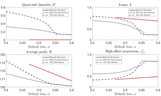
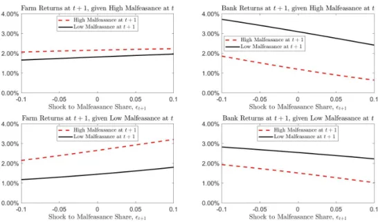
2.3 Varying Bank Capital,k. . . 43 2.4 Varying the Default Loss Rate, α. . . 44 3.1 Annualized Returns at t+ 1 Conditional on the Shocks to the
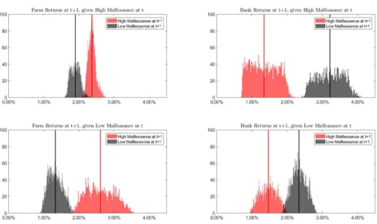
Mean Malfeasance Share att+ 1 . . . 66 3.2 Histograms of Realized Returns conditional on Mean
Malfea-sance State, ¯ms. . . 67
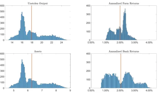
3.3 Histograms of Assets, Non-Stolen Output and Returns to
Bank-ing and FarmBank-ing . . . 68 3.4 The Economy’s Transition – High to Low to High Mean
Malfea-sance. . . 70 3.5 The Economy’s Transition – Low to High to Low Mean
Malfea-sance. . . 70 3.6 Transition to High Mean Malfeasance after Extended Low Mean
Malfeasance . . . 71 3.7 Baseline Transition . . . 72 3.8 Economy’s Transition With and Without Deposit Insurance. . . . 73 3.9 An Example Transition With and Without Monitoring . . . 79 3.10 The Effect of Free Reports on Monitoring Expenditure . . . 80 3.11 Economies with Low and High Disclosure and Deposit Insurance. 81
3.12 Comparing Means of Aggregates in Different Regimes. . . 83
3.13 Comparing Variability of Aggregates in Different Regimes. . . 84
4.1 SOMA . . . 94
4.2 QE and Balances at Bank of England, authors’ calculations . . . . 100
4.3 M4 and QE, authors’ calculations . . . 101
4.4 Breakdown of US repayments . . . 105
4.5 Breakdown of US repayments, excluding GSEs . . . 105
4.6 USA monthly . . . 106
4.7 GSE graph . . . 106
4.8 Winners$bn . . . 107
4.9 Winners, excluding fees from insurance guarantees$bn . . . 108
4.10 Losers, excluding fees from insurance guarantees $bn . . . 108
4.11 Losers$bn. . . 109
4.12 Breakdown of UK repayments . . . 110
4.13 UK monthly. . . 111
4.14 Real return on bank equity for US participants of bank recapi-talization programs. . . 112
4.15 IRF results comparing slow recovery with government support to a ‘short sharp shock’ without. . . 120
List of Tables
2.1 Parameter Values . . . 39
2.2 Implied Deposit Limits and Effort Levels . . . 39
2.3 Welfare Comparisons . . . 41
3.1 Parameter Values . . . 62
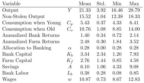
3.2 Average Values in Model’s Stochastic Steady State . . . 64
3.3 Average Values when Mean Malfeasance Share is Low att. . . 64
3.4 Average Values when Mean Malfeasance Share is High att . . . 65
3.5 Path oft for First Ten Periods of Transition . . . 72
3.6 Average Values with Deposit Insurance . . . 74
3.7 Effect of Information on Allocation to Banking. . . 78
3.8 Average Values with Monitoring . . . 79
3.9 Average Values with Low levels of Disclosure, φ= 0.2 . . . 82
3.10 Average values with High Levels of Disclosure,φ= 0.4 . . . 82
3.11 Percentage Compensating Variations . . . 84
4.1 QE in the USA. * indicates authors’ calculations. . . 103
4.2 Net gains (losses) from the UK recapitalization program, £m . . . 110
4.3 Parameter Values . . . 119
Introduction
We introduce and motivate the class of problems considered in this thesis and survey the relevant economics literature
At the end of their seminal book on bank regulation (Dewatripont, Tirole, et al. (1994)), the authors lay down a challenge for future research. As de-posit insurance reduces incentives for savers to monitor bank risk, what would happen if insurance were restricted to only cover safe assets? This is a sys-tem known as narrow banking1 – in contrast with the dominant policy2 of ‘blanket’ coverage which does not restrict how insured deposits are invested. That the question remains unanswered speaks to the many facets that must be considered. A major challenge is the central role that banks play in the provision of both liquidity and credit. Both services link banks to the real economy – an area that has received intense attention since the Global Finan-cial Crisis (GFC). Morley (2016) provides an excellent summary of the vast literature that has emerged. However, discussion of changes to the scope of deposit insurance has been limited, with notable exceptions from King (2016); Lilico (2010); Dowd (2013); Calomiris and Haber (2014) and Kotlikoff (2010).
1
First suggested by Fisher (1935), as ‘the Chicago Plan’, narrow banking has been supported by many economists (Hart (1935); Tobin (1987); Friedman (1960)) and is enjoying a recent resurgence (Kay et al. (2010); Benes and Kumhof (2012); Pennacchi (2012)).
2
Demirg¨u¸c-Kunt, Kane, and Laeven (2014) document the geographic scope and extent of deposit insurance worldwide.
Naturally, there is variation in opinion on the optimal alternative policy.3 Regulatory change – especially for policies which directly connect savers to bank risks4 – requires a burden of proof in the form of a substantial literature. This thesis takes a general stance on the form of the alternative system and is most concerned with providing theoretical results for a policy regime in which deposit insurance is restricted or removed completely. In particular, we focus on the ability for such a system to provide liquidity and credit.
Holmstrom (2015) defines a liquid asset as one that can be sold at face-value ‘no questions asked’ (NQA). Such assets are useful for transactions and trade with a liquidity premium (Stein (2012); Krishnamurthy and Vissing-Jorgensen (2012)). Chapter 2 focuses directly on liquidity provision in a simple micro-theory framework where banks can choose to exert monitoring effort to improve loan quality. We show that, relative to deposit insurance, the government can provide commensurate liquid assets by issuing government debt directly to narrow banks. In terms of lending, deposit insurance provides the highest quantity of loans but of a lower quality, relative to the case of narrow banking.
Townsend (1979) models the agency problem between a bank and an en-treprenerial borrower, where the entrepreneur has incentive to falsify returns. Chapter 3 uses an overlapping generations model to consider the same prob-lem between savers and the bank. The long generational time-frame abstracts from liquidity issues thus this Chapter can be understood as focusing on the
3
Miron (2010) and Dowd (1992, 2013) come from a libertarian stance prefering a fully free-market solution, while King (2016) provides a transitional policy ceding greater power to the central bank. Kay et al. (2010) would allow narrow banks to invest in residential mortgages. Kotlikoff (2010) and Cochrane (2014) restate the policy of Jacklin (1989) of using equity-funded banking. Pennacchi (2012) points out the equity suffers from ‘cream-skimming’ (Gorton and Pennacchi (1990)) and the traditional definition of a narrow banking system which provides debt layered on government bonds is preferable for transactions.
4
Another cause for concern is the re-introduction of ‘sunspot’ bank runs as in Diamond and Dybvig (1983). Jacklin (1989) and Dowd (2000) point out runs are a problem linked to insufficient capitalization.
‘wide’ sector of a narrow-wide banking system. We note the problems in charg-ing actuarially fair insurance premia (Leonard (2013); Chan, Greenbaum, and Thakor (1992)) and assume that, in a crisis, government funds are necessary to ensure depositors are repaid in full. We show that if these funds are instead spent preventing the “cream-skimming” problem with equity savings contracts (Gorton and Pennacchi (1990)) then equity-funded banking can provide signif-icant welfare improvements. Using government funds to promote bank disclo-sure contrasts with the proposal in Dang, Gorton, Holmstr¨om, and Ordo˜nez (2017) who argue that bank opacity is necessary for liquidity. We point out that government debt is an ample source of safe liquid assets for transactions. Opacity creates hard-to-measure risk. It is far simpler for governments to au-dit a transparent banking sector than a deliberately over-complicated one. We also consider investor-funded ratings unions but these suffer from the para-dox that costly information suffers from free-riding (Grossman and Stiglitz (1980)).
It is common for large industries to extract government assistance when hit with potentially catastrophic losses. The scale, however, of assistance given to banks following the crisis was extraordinary. Chapter 4 attempts to quantify the real cost of bank recapitalization in the US and UK. Contrary to Treasury reports, our figures include inflation and the effect of Quantitative Easing on government costs of borrowing incurred from funding the emergency recapitalization of banks. The key finding is that differences in the treatment of equity-holders of recipient banks changed the outcome of the programes. The treatment of equity-holders of receipient banks was not consistent. In the UK, Northern Rock’s shareholders received no compensation when the bank was nationalized, while the Royal Bank of Scotland and Lloyds Bank suffered no dilution despite the government taking a majority stake in each company. In the USA, all profits from Government Sponsored Enterprises – Fannie Mae and Freddie Mac – are transferred to the government, at the expense of its
shareholders. Without this ruling, the headline result that the Troubled Asset Relief Program (TARP) was profitable disappears. All other recipients were not subject to this ongoing profit transfer. Other differences between the two countries result from the lessons that the US regulators learned from the UK programme. Chiefly, US regulators mandated that recipient banks issue warrants so the taxpayer benefitted from capital gains. Secondly, the US program was able to corral a large number of healthier banks to join the program, which raised average returns. The UK results are dominated by the large losses which will result from the eventual sale of the government’s stake in the Royal Bank of Scotland.
Chapters 2 to 4 form the core of the present thesis. Chapter 2 is based on a paper authored with George Pennacchi. Chapter 3 is based on a paper co-authored with Lawrence Kotlikoff. Chapter 4 is based on a paper co-co-authored with Huw Dixon. Chapter 5 concludes.
How Should Governments
Create Liquidity?
Governments can create safe, liquid assets by issuing government debt or by insuring private debt, such as bank deposits. Yet this public liquidity creation is limited by the government’s capacity to raise taxes to pay its liabilities. This paper analyzes the effects of safe asset creation in a financial system where individuals es-pecially value default-free assets. It compares a banking system with fairly-priced deposit insurance to banking systems with both uninsured “broad” banks and “narrow” banks which invest only in government debt. We find that a system with deposit insurance maximizes the amount of bank system lending but leads to less ef-ficient monitoring of bank borrowers. The alternative system with narrow and broad banks produces the same amount of government safe assets but more privately-created “quasi-safe” assets.
2.1
Introduction
This paper analyzes the design of a country’s banking system when its govern-ment’s taxing capacity limits the amount of safe assets that can be created.
A government can provide safe (default-free) assets by insuring bank deposits or by directly issuing government debt, such as Treasury bills. Yet it can do so only to a limited degree. A government’s total liabilities are constrained by the amount of taxes that it can raise from its citizens.
We compare a system where the government provides limited deposit in-surance to banks that make risky loans versus a system where the government requires that narrow banks invest only in the government’s directly issued debt (Treasury bills) and uninsured “broad” banks make risky loans. In both systems, safe assets may be created by the government but “quasi-safe” assets can also be created privately. The distinction between government safe assets and private quasi-safe assets is that the former are fully default-free while the latter are default-free except during a severe financial crisis or “catastrophe.” Individuals are willing to pay “liquidity” premiums to invest in safe assets, where the premium is greater for fully-safe assets compared to quasi-safe as-sets. Because individuals especially value liquidity, they accept lower rates of return on safe assets relative to the certainty-equivalent return on risky assets. The banks in our model are local and separated, with similarities to the ‘islands’ models developed in Lucas Jr (1972, 1975), such that interbank net-work effects are precluded. Our model assumes that banks can improve the returns on their risky loans by costly monitoring of their borrowers. How-ever, monitoring is not contractible so that the bank’s owner-manager must be given incentives to monitor efficiently. Because the bank owner has limited liability, the bank’s choice of leverage (deposit-to-equity capital ratio) affects its incentive to monitor. A bank that limits its leverage can signal its incentive to efficiently monitor, which can raise the bank’s firm value and potentially lower its cost of deposit funding. Because monitoring costs are assumed to vary across banks, in general some lower-cost banks may limit leverage and
0Compared to deposit-insured banks, uninsured broad banks might be considered a type
efficiently monitor while other higher-cost banks choose high leverage and do not monitor. Our model also permits a bank to issue deposits with different seniorities, a process referred to as “tranching.” For some banks, issuing both senior and junior deposits can be profitable because the former can be made quasi-safe.
We use the model to investigate three regimes: a baseline, fully-private banking system with no government safe assets; a scheme of fairly-priced government deposit insurance; and a system combining narrow banks that invest in government debt and uninsured broad banks that make loans. We assume the tax base available to finance a government’s safe assets is identical in the latter two regimes to allow for a fair comparison.
We show that the creation of safe assets that derives from the government’s ability to impose future taxes can potentially improve welfare by providing more and higher-quality liquidity. However, government safe asset production can come at the cost of less-efficient bank monitoring or less total bank lending. Government deposit insurance is profitable for banks because deposits that are completely safe, even during a catastrophe, are especially valued by savers and require the lowest risk-adjusted rate of return. However, sufficiently high levels of deposit insurance reduce the amount of efficient monitoring in the banking system and can crowd out quasi-safe deposits.
In a system with narrow banks and uninsured broad banks, narrow banks that take deposits and invest in government debt may, in some structures, reduce the deposits available to broad banks that make loans. As a conse-quence, banking system lending can decline. However, because fewer deposits limit the leverage of broad banks, the lending that does occur tends to be done with more efficient monitoring and possibly greater production of quasi-safe deposits. However, under a different narrow bank - broad bank structure,
narrow banks would not reduce deposits available to broad banks and would be equivalent to a system of fully-private lending banks but with the benefit of additional government safe assets.
Our paper contributes to a literature on the private and public provision of safe assets.1 Prior research, including Gorton and Pennacchi (1990) and Dang, Gorton, Holmstr¨om, and Ordo˜nez (2017), notes that safe assets are especially valuable for making transactions due to their information-insensitivity. The “money-like” feature of safe assets can allow them to pay a lower rate of return compared to riskier, less-liquid assets. Such a liquidity premium is empirically documented by work including Krishnamurthy and Vissing-Jorgensen (2012), Sunderam (2015), and Nagel (2016).
Research shows that safe assets can be created privately via financial insti-tutions such as banks (e.g., Diamond (2017)) or special purpose vehicles that invest in risky debt and issue tranched securities (e.g., DeMarzo and Duffie (1998) and DeMarzo (2005)). However, safe assets can also be created by gov-ernments in the form of sovereign debt or by insuring privately-issued debt, such as bank deposits (e.g., Greenwood, Hanson, and Stein (2015), He, Kr-ishnamurthy, and Milbradt (2018), Gatev and Strahan (2006), and Pennacchi (2006)).
Most papers that analyze the co-existence of private and public safe assets concentrate on issues related to financial stability. Research by Holmstr¨om and Tirole (1998), Bolton, Santos, and Scheinkman (2009), and Stein (2012) present models where the provision of government safe, liquid assets can im-prove financial system stability relative to an economy with only private liquid assets.
Our paper also analyzes the interaction between private and public safe
1
assets, but our focus relates to issues of lending efficiency and the aggregate volume of private safe assets. As in Diamond (1984), banks in our model can create value by making loans and providing costly monitoring of borrowers. We study how theform of government safe assets affects monitoring efficiency and private liquidity creation. Our paper’s main contribution is to show that public safe assets in the form of government-insured deposits can have differ-ent implications compared to public safe assets in the form of directly-issued government debt. They have different effects with regard to a banking sys-tem’s aggregate lending, its lending efficiency, and its creation of private safe assets.
The next section introduces our basic model and considers a fully-private banking system with no role for government. Section 3 examines a banking system with government deposit insurance that is limited by the government’s capacity to tax agents’ future wages in order pay insurance losses. Section 4 considers a banking system where the government directly issues debt that is held by narrow banks that operate like “Treasury-only” money market mutual funds. In this system, uninsured broad banks make loans. As with deposit insurance, the amount of government debt that can be issued is limited by the government’s future taxing capacity. Section 5 provides numerical illustrations of the model’s results, and Section 6 briefly discusses the robustness of the model’s assumptions. Conclusions are given in Section 7.
2.2
Liquidity Creation in a Fully-Private Banking
System
This section presents our basic model of a private banking system that has no role for a government to create safe assets. Private banks can create only quasi-safe assets, which are default-free except in a financial catastrophe. The following sections will consider how a government can create fully default-free
assets due to its ability to tax individuals’ future endowments.
Consider a single-period economy with risk-neutral agents who obtain util-ity from their end-of-period consumption. Agents receive initial endowments that can be transformed into end-of-period consumption using two types of investment technologies. One is a risky investment technology that is available to all agents. The other is a superior risky investment technology that can only be accessed through lending intermediaries, which we call “banks.”
There are two types of agents: agents who are capable of owning and managing banks and other agents who wish to save and value liquidity derived from investing in safe assets. We will refer to the former agents as “bankers” and the latter agents as “savers.” Each banker has a fixed beginning-of-period endowment of inside equity equal tok. A banker can raise additional funds in the form of deposits from its local savers who can deposit only in their local bank.2 We normalize the maximum amount of available local savings to 1 and the amount of total deposits actually issued by the bank is denoted by γ ≤1. Therefore, a bank’s beginning-of-period assets equals (γ+k)≤(1 +k).3
Banks are special due to their superior lending technology that funds iden-tical projects in perfectly elastic supply. All projects, and therefore loans, are subject to only aggregate (macroeconomic) risk.4 We consider three end-of-period states of the world: ‘good,’ ‘bad,’ and ‘catastrophe.’ The good state occurs with probability pg, in which case each loan’s end-of-period return per
unit lent equals its promised return of RL. The bad state occurs with
prob-ability pb, in which case each loan defaults but has a positive recovery value.
2
Savers are limited to investing only in the bank’s debt (deposits) and not its equity. In richer models where savers cannot verify the return on the bank’s assets or have needs to trade, they may prefer bank deposits relative to bank equity. For example, see Diamond (1984); Townsend (1979); Gorton and Pennacchi (1990).
3As will become clear, a banker has the incentive to invest the entire amount of capital,
k, in the bank because of its access to a superior investment technology.
4We focus on macroeconomic risk because, in general, idiosyncratic risks might be
Finally, the catastrophe state occurs with probability pc = 1−pg −pb, in
which case the loan defaults and has a zero recovery value.
The banker is able to improve each loan’s recovery value in the bad state by exerting beginning-of-period effort to monitor the borrower.5 This recovery value is denoted by d(a), where a is a banker’s beginning-of-period level of effort per unit of loan. Recovery value per unit of loan is assumed to be the following increasing and concave function of banker effort:
d(a) =RL
1−αe−βa
(2.1) where 0 < α < 1 and β > 0. Monitoring effort is assumed to be costly in terms of diminishing the banker’s utility at a fixed marginal cost per unit of effort.6 Denote Banker i’s marginal cost of effort by ci. We assume the
country’s economy has a continuum of local bankers who differ in terms of their cost of monitoring, where ci belongs to a continuous distribution having
the range:
ci∈[pbβ(RL−1), pbαβRL]≡[c,c¯]. (2.2)
As will be shown, this restriction on the range of monitoring costs ensures that each bank’s first-best effort is positive but still results in a positive loss given default. Importantly, it is also assumed that each bank’s effort level, a, is unobservable to savers and, hence, cannot be contracted upon.
While savers are risk neutral, they have an additional ‘liquidity’ demand for safe assets. Savers have direct access to a risky investment technology that funds projects in perfectly elastic supply and pays a return per unit investment ofRR/pgonly in the good state. Therefore, this non-intermediated investment
5
We refer to this effort as monitoring, but it could also be interpreted as credit screening to determine which loan applicants have higher recovery value.
6
Alternatively, one could assume bankers differ in terms of how efficient is their effort in improving recovery value,β.
technology has an expected return per unit investment ofRR< RL.7 However,
savers will accept the expected return of RC < RR on an investment that is
default-free in the good and bad states but not the catastrophe state. Thus, this ‘quasi-safe’ investment does not default with probability ℘≡pg+pb and
defaults with probability pc = 1−℘. Examples of these investments might
include money market instruments such as A1/P1-rated commercial paper and wholesale, uninsured bank certificates of deposit.8 Later we will consider government-created assets that are default-free in all states for which savers require a return that is even lower than RC. As in Stein (2012), we assume
that savers’ required return on quasi-safe assets is independent of their supply. We can define a quasi-safe asset’s liquidity premium bylwhereRC(1+l) =
RR. This liquidity premium can be considered a utility bonus due to a safe
asset’s value in settling transactions and for use as collateral.9
Because loans return zero in the catastrophe state, the best that a private bank can do is to create quasi-safe deposits. Doing so allows it to reduce its cost of funding by the liquidity premium l. The bank can augment its quasi-safe deposits in two ways. One way is by increasing the recovery value of its loans in the bad default state by efficiently monitoring its borrowers. However, for depositors to find this credible, the bank must have an incentive to undertake this unobserved action. The bank can create this incentive by restricting its leverage so that bank equity receives the marginal benefit from its costly monitoring effort.
7
These projects may be the same types of projects that banks fund with loans. However, savers are not able to monitor borrowers and obtain inferior expected returns relative to those received by banks.
8This asset class might be considered a ‘near-money’ or what Moreira and Savov (2014)
refer to as ‘shadow money.’
9
Gorton and Pennacchi (1990) provide a theory for why safe assets are particularly valuable for transactions. Several recent models, such as Stein (2012), assume that the moneyness feature of safe short-term gives it a lower required return than the certainty-equivalent return on risky assets.
The second way that a bank might increase its quasi-safe deposits is by “tranching” its debt, which means that it issues both senior deposits and junior deposits (or subordinated debt). Designed appropriately, the senior deposits can be made quasi-safe and supported by the additional assets that are funded by junior deposits. We defer consideration of tranching until the next section. For now, we assume that the bank issues only a single class of deposits of the amount γ.
Bankers are assumed to be the only equity investors (shareholders) of the bank. Their profit-maximizing choice of leverage and effort may result in savers’ deposits being either quasi-safe or default-risky. We now consider the possible equilibrium behavior of these limited-liability bankers and savers.
An equilibrium is defined as follows. First, a bank(er) announces that it will raiseγ ≤1 in deposits, so that its total assets equalsγ+k. Second, given this choice of leverage (deposits and total assets), the bank’s promised return on deposits, RD, is set. Third, given this deposit rate, the bank chooses its
unobserved effort level,a. An equilibrium is a choice ofγandathat maximizes the bank’s profits and a promised deposit rate RD that satisfies depositors’
participation constraint given the bank’s announced γ and its equilibrium profit-maximizing choice of a.
Since Bank ihas monitoring costci, its profit maximization problem can
be characterized as: max
γ,a pg[(γ+k)RL−γRD]+pbmax [(γ+k)d(a)−γRD,0]−cia(γ+k) (2.3)
subject to the constraint that its deposits cannot exceed 1:
and subject to depositors’ participation constraint: RD ≥ RR−pbγ+γkd(a∗) pg if (γ+k)d(a ∗)< γR C/℘ RC/℘ otherwise (2.5)
Note that the expected profits given in (2.3) reflect the fact that the bank may or may not default in the bad state but will always default in the catastrophe state due to loans’ zero recovery value in that state. Also, the depositors’ participation constraint (2.5) reflects either default in the bad state (the first line on the right-hand side) or no default in the bad state (the second line on the right-hand side). In the former case, depositors’ required expected return is RR, but in the latter case it isRC since deposits are quasi-safe.
The solution to the problem can be found by noting that whenever default occurs in the bad state, (γ +k)d(a∗) < γRC/℘, then from the objective
function (2.3) we see that the banker receives no benefit from monitoring and the bank’s private effort choice will be a∗ = al ≡ 0. Deposits’ equilibrium promised return must then be RD =
RR−pbγ+γkd(al)
pg =
RR−pbγ+γkRL(1−α)
pg and
the bank’s expected profit is
πl=pg[(γ+k)RL−γRD] = (γ+k)[pgRL+pbRL(1−α)]−γRR. (2.6)
Instead, whenever (γ+k)d(a∗)> γRC/℘so that the banker obtains a return
in the default state, then its optimal choice of effort will either be the same corner solutional= 0 or the effort level implied by the first-order condition:
∂d(a)
∂a = ci
pb
. (2.7)
By substituting in the functional form for d(a) from equation (2.1), the effort satisfying this first order condition is a∗=ah where
ah≡ 1 β ln βαpbRL ci (2.8) which results in the loan’s bad state recovery value equaling
d(ah) =RL−
ci
βpb
In this case deposits are quasi safe, RD =RC/℘, and the high-effort bank’s expected profit is πh= (γ+k) h pgRL+pbd(ah)−ciah i −γRC (2.10)
where pbd(ah)−ciah > pbRL(1−α) is the expected recovery value net of
monitoring costs. Thus, al = 0 or ah given by equation (2.8) are the only choices of effort that could possibly be profit-maximizing for the bank. The following lemma states that a bank’s profit-maximizing choice of effort, and its equilibrium deposit interest rate, depends on whether its initial choice of leverage is below or above a particular threshold value which we refer to as
γm.
Lemma 1. If Bank i chooses initial deposits less than or equal to γm(ci) ≡
k pbd(ah)−ciah
RC/℘−(pbd(ah)−ciah), then the equilibrium is one where the bank supplies
first-best effort (2.8), RD =RC/℘, and has profits equal to equation (2.10). If it
chooses initial deposits exceeding γm(ci), the equilibrium is characterized by
no bank effort, RD =
RR−pbγ+γkRL(1−α)
pg , and profits equal to equation (2.6). The proof in given in Appendix A. Thus, the profit function is given by equations (2.6) and (2.10), where the switch point occurs at γ = γm. The bank’s profit maximizing choice of γ is then the maximum of this profit func-tion. As both profit functions, (2.6) and (2.10), are linear and increasing inγ, these maxima are at the endpoints, γ =γm and γ = 1 respectively.10 Banks simply compare profits at
πl=(1 +k) [pgRL+pbd(0)]−RR (2.11)
πh =(γm+k)hpgRL+pbd(ah)−ciah
i
−γmRC (2.12)
and choose the (γ, a) combination (γm, ah) if πl ≤ πh and otherwise choose (1,0).
10
We rule out parameter values for which profit is decreasing inγsince that implies that banks choose to issue zero deposits.
Now note from (2.11) and (2.12) thatπl does not depend on the banker’s
cost of effort, since no effort is expended. Moreover, πh is a monotonically decreasing function of the banker’s cost,ci.11 Assuming that
πh(¯c)< πl< πh(c), (2.13) then there exists a unique c∗ that is the value of c such that πl = πh. It satisfies the implicit equation:
c∗ = π lp b(RL−RC/℘) 1 β +ah(c∗) (πl−p gkRC/℘) (2.14) where ah(c∗) = β1ln βαpbRL c∗
. This logic leads to the following proposition that is proven in Appendix A.
Proposition 1. If Bank i’s cost of monitoring isci < c∗, it chooses leverage
equal to γm(ci), provides first best effort of ah(ci), sets RD = RC/℘, and
has profits equal to equation (2.12). Instead, if its cost is ci > c∗, it chooses
γ = 1, provides no effort, setsRD = RR−pb(1+pkg)RL(1−α), and has profits equal
to equation (2.11).
Thus, only low monitoring cost banks, defined as having ci < c∗, limit
leverage, provide first-best effort, and create quasi-safe deposits.
Our results to this point assume that a bank issues only one class of de-posits. The next section considers whether a bank might choose to issue both senior deposits and junior (subordinated) deposits. Interestingly, the process of tranching deposits can permit issuance of quasi-safe deposits by high-cost, no-effort banks.
2.2.1 Tranching
Consider a bank that offers two classes of deposits: senior deposits and junior deposits (or subordinated debt). Suppose that the bank restricts the amount
of its senior deposits,γs, such that it has sufficient loan recovery value in the
bad default state to pay off senior depositors in full. Intuitively, the bank may have an incentive to do so because it ensures that senior deposits are quasi-safe and their promised return is relatively low at RC/℘. In addition,
let the amount of junior deposits be γj and their promised return be R D,j.
For an equilibrium effort level, a, the amount of senior, quasi-safe debt that the bank could issue,γs, will satisfy:
(γs+γj+k)d(a)≥γsRC/℘ (2.15)
or, equivalently, senior leverage must be below a maximum, ¯γs, which is
in-creasing in effort, a, and other forms of bank funding, γj+k,
γs≤γ¯s≡ (γ
j +k)d(a)
RC/℘−d(a)
. (2.16)
The bank’s profit maximization problem is now characterized as: max γj,γs,a pg (γs+γj+k)RL−γsRC/℘−γjRD,j (2.17) +pbmax (γs+γj +k)d(a)−γsRC/℘−γjRD,j,0 −ca(γs+γj+k) subject to the constraint (2.15) that senior deposits are quasi-safe and subject to junior depositors’ participation constraint:
RD,j ≥ RR−pbγj[(γs+γj+k)d(a∗)−γsRC/℘] pg if (γ s+γj+k)d(a∗)−γsR C/℘ < γjRC/℘ RC/℘ otherwise (2.18) To solve this problem, let us start by considering the bank’s incentive to exert effort. Note that bank equity benefits from effort only if it receives the marginal profit from effort in the bad default state. That can only occur when (γs+γj+k)d(a)−γsRC/℘−γjRD,j >0. (2.19)
But if inequality (2.19) holds, then junior deposits are also quasi-safe, can be paid a deposit interest rate of RD =RC/℘, and are no different from senior
deposits. Consequently, a bank that monitors at first best, a∗ = ah, cannot
benefit from issuing more than one class of (senior) deposits. Thus, if a bank has a relatively low cost of exerting effort so that its optimal effort choice is first-best, then optimal effort, leverage, and profits are{ah, γm, πh}, the same as when it does not tranche.
Instead, consider a bank that has relatively high monitoring costs such that it is optimal not to exert effort and inequality (2.19) does not hold. Without tranching, Proposition 1 shows that this bank would choose maximum lever-age,γ= 1, and all deposits suffer losses in the bad default state. Consequently, the bank’s per unit expected cost of deposit funding is RR. Tranching now
allows the bank to reduce part of its deposit funding costs. Since quasi-safe senior deposits have the lower per unit expected cost of RC < RR while the
expected cost of junior deposits is unchanged at RR, the bank has the
incen-tive to issue the maximum amount of quasi-safe senior deposits,γs= ¯γs. As a result, junior deposits receive nothing in the bad state so that their promised return is RD,j = RpRg .12
Since a bank that chooses no effort, al = 0, profits by maximizing to-tal leverage, γ = 1, even when it does not tranche its deposits, its profit-maximizing amount of junior deposits is γj = 1−¯γs. Thus, tranching does not affect this bank’s equilibrium effort or total leverage, but permits it to create quasi-safe assets equal to
γs= (1−γ s+k)R L(1−α) RC/℘−RL(1−α) = (1 +k)RL(1−α) RC/℘ (2.20) Doing so yields increased profits as a result of the reduced funding cost of senior deposits. Denoting the no-effort bank’s profits under tranching as πTl,
12
The fact that in equilibrium junior deposits receive nothing in the bad state makes their payoff similar that of the banker’s inside equity,k. In this sense, junior deposits might be considered similar to outside equity. However, the effort incentive of the banker depends his/her inside equity, so issuing more junior deposits is not equivalent to the banker starting with more inside equity.
we have πTl =pg (1 +k)RL−γs RC ℘ −(1−γ s)RR pg =(1 +k) [pgRL+pbRL(1−α)]−γsRC−(1−γs)RR =(1 +k) [pgRL+ (pb+℘l)RL(1−α)]−RR, (2.21)
where recall that the liquidity premium,l, is defined byRR= (1+l)RC.
Com-pared to profits without tranching in equation (2.11), we see that tranching raises the no-effort bank’s profits by the liquidity premium that it saves on its quasi-safe senior deposits:
πTl −πl=℘l(1 +k)RL(1−α) =lγsRC ≥0.
This increase in no-effort profits alters the monitoring cost threshold above which banks choose no effort. By equating πlT in equation (2.21) to πh in equation (2.12), the critical value of ci is now:
cT = π l Tpb(RL−RC/℘) 1 β +ah(cT) (πlT −pgkRC/℘) . (2.22)
Since πlT > πl and pgkRC/℘ >0, we see thatcT < c∗. Intuitively, tranching
deposits makes choosing no effort relatively more profitable than choosing high effort. Hence, there is a lower cost threshold at which banks choose no effort. We summarize these results in the following proposition:
Proposition 2. If Bank i’s cost of monitoring is ci < cT, it does not benefit
from tranching and its leverage, effort, deposit rate, and profits are the same as without tranching. Instead, if its cost is ci > cT, it exerts no effort and
issues senior deposits of γs and junior deposits of 1−γs where γs is given
by equation (2.20). The deposit rates of senior and junior deposits are RC/℘
and RR/pg, respectively, and the bank’s profits are given by equation (2.21).
Since, cT < c∗, more banks choose no effort when tranching is possible than when it is not.
It is interesting to note that if banks are not permitted to tranche deposits, low-cost, high-effort banks are the only ones that can produce quasi-safe de-posits. However, if tranching is permitted, now high-cost, no-effort banks create quasi-safe deposits and, moreover, the amount that they create can exceed that of the low-cost, high-effort banks. That is, there are parameter values such that γs> γm(ci) for a range of ci < cT. It may seem ironic that
high-cost banks which do not monitor and have riskier loan portfolios are able to create more quasi-safe deposits. Of course they do so by issuing more risky junior deposits because they need not signal their incentive to monitor by having low total leverage. The next section considers the aggregate amount of quasi-safe assets produced by a private, uninsured banking industry.
2.2.2 Quasi-Safe Asset Production
The provision of quasi-safe, liquid assets may be considered a key measure of social welfare. Let f(ci) be the economy’s density of bankers with monitoring
cost ci. Then assuming tranching is permitted, the quantity of quasi-safe
deposits produced by banks that choose first-best effort is Z cT
c
γm(ci)f(ci)dci, (2.23)
where each bank that exerts first best effort issues quasi-safe deposits equal to γm(ci) =k
pbd(ah(ci))−ciah(ci)
pbRC/℘−[pbd(ah(ci))−ciah(ci)] and where the high effort - no effort monitoring cost threshold, cT, is given by equation (2.22).
Each no-effort bank issues quasi-safe, senior deposits equal to γs given by equation (2.20). Thus, total quasi-safe deposit production combines both the high-effort banks’ total deposits and the no-effort banks’ senior deposits. Denoting the economy’s total quasi-safe deposits under tranching as Sc
T, it satisfies STc = Z cT c γm(ci)f(ci)dci+γs Z ¯c cT f(ci)dci. (2.24)
Assuming a uniform density for monitoring costs, equation (2.24) simplifies to STc = 1 ¯ c−c " Z cT c γm(ci)dci+γs(¯c−cT) # . (2.25)
Since quasi-safe deposits are vulnerable to losses in the catastrophe state, there is the potential for a government with taxing authority to improve welfare by producing assets that are safe in all future states, including severe crises. The next section considers this possibility by way of government deposit insurance.
2.3
Liquidity Creation with Government Deposit
Insurance
In this section, we first discuss a feature that can give a governmental advan-tage to producing safe assets, namely, the government’s ability to tax sources of income that may not be available to private creditors. We then consider the particular case of government-backed bank deposits.
2.3.1 Taxes as a Source of Public Liquidity
Relative to private entities, a government’s power to tax can give it an advan-tage in producing safe assets. In particular, a government might raise revenue from sources of income that may be difficult to pledge under private contracts. Future revenue from human capital, i.e., wage income, may be an example. Payment from an individual’s future wages may be difficult to collect under private contracts due to bankruptcy laws that provide limited protection to private creditors. Compared to the rights of private creditors, a government typically is in a stronger position to collect taxes that are owed.
We model a government’s taxing authority by assuming that savers receive end-of-period wage income that is riskless and equal toωper unit of
beginning-of-period savings.13 These wages are not pledgeable under private contracts, but a government is able to tax a proportion ¯t≤1.14 This taxable proportion might be determined by moral hazard considerations: if the tax rate is too high, individuals may have an incentive to evade taxes.15
The government’s taxing capacity gives it the ability to create assets that are default-free, even in the catastrophe state. Examples might include Treasury debt, such as Treasury bills, and government-insured debt or de-posits. These assets’ moneyness and liquidity are assumed to be particularly attractive to savers such that perfectly safe assets’ required return equals
RF where RF < RC < RR. Written in terms of liquidity premia, we have
RR= (1 +l)RC = (1 +l)(1 +lf)RF. Thus, increasing safety is associated with
higher liquidity premia that reduce the returns required by savers.
The next section considers one way that a government can create a fully-safe asset, namely, deposit insurance. Following that, we consider fully-safe asset production by a government that issues its own debt.
2.3.2 Deposit Insurance
Suppose that the government offers fairly-priced deposit insurance to private banks that permits insured deposits to be default-free in all end-of-period states, including both the ‘bad’ and ‘catastrophe’ states when loans default. Since deposit insurance is backed by the government’s power to tax savers’ end-of-period wages, the amount of these taxes is state-contingent. Yet for deposit
13
Our results are not sensitive to the assumption that wage income is riskless. What matters is that there is some strictly positive minimum level of wages that can be taxed even in the catastrophe state.
14If wages could be pledged under private contracts, individuals could underwrite
insur-ance against a bank’s default on its deposits; that is, savers could provide credit protection. Or, alternatively, individuals could issue riskless debt at the beginning of the period backed by their future wages. Both actions could increase the amount of safe assets.
15
A similar, but alternative, assumption would be to have a direct cost to raising taxes that is increasing and convex in the amount raised. This cost would subtract from social welfare.
insurance to be fully credible, it must insure deposits in case of catastrophe when each bank’s assets are worthless. This worst-state scenario limits insured deposits to equal the government’s maximum revenue that can be raised in taxes at the end of the period.
We assume that the insurer limits its maximum liability by restricting the quantity of deposits that it will insure at each bank. One can imagine that this policy is implemented by limiting insurance to small “retail” deposits, assumed to equal a proportion γr of total savings in each banking market. Consequently, we assume the maximum promised end-of-period payment to insured depositors is γrRF for each bank.
Because our intent is to study the potential amount of safe assets that a government can create with deposit insurance, we do not consider the well-known distortions due to insurance mis-pricing.16 Rather, we assume the government assesses a fair insurance premium payable by the bank at the end of the period, whereφ is the premium per promised payment on insured deposits.17 Specifically, if a bank chooses to issue the maximum amount of insured deposits, then its total promised payment to insured depositors and the deposit insurer is γrR
F(1 +φ). Because deposit insurance is fairly priced,
the premium φwill vary across banks based on their default risk.
Not all banks may choose to issue the maximum amount of insured de-posits. A bank’s equilibrium choice can depend on its individual cost of mon-itoring, ci. We begin by taking as given the government deposit insurance
limit of γr for each banking market and determining an individual bank’s profit-maximizing choice of insured deposits. Then we will aggregate over all
16While extensive empirical evidence suggests deposit insurance is typically under-priced,
it is possible that a government might want to set higher-than-fair deposit insurance premi-ums in order to capture the liquidity premium from its creation of fully-safe assets. Since governments do not seem to embrace this practice, we leave this issue for future research.
17
We assume the premium is distributed as a lump sum payment to savers in the good state.
banking markets to determine the maximum level ofγrthat can be supported
by the government’s taxing power. High Cost Banks
Recall that in the absence of deposit insurance, banks with relatively high monitoring costs choose maximum leverage (γ = 1), zero effort (al = 0), and tranche their deposits such that the promised payment on senior deposits equals the bank’s asset return in the bad state (γs given by equation (2.20)). In equilibrium, these banks’ expected cost of quasi-safe senior deposits is RC
and their expected cost of junior deposits isRR.
For the sake of both simplicity and realism, we assume that the maximum amount of insured deposits,γr, is such thatγrRF ≥γsRC/℘= (1 +k)RL(1−
α). In other words, the maximum promised payment on insured deposits exceeds the no-effort bank’s asset return in the bad state. Thus, if this bank issues the maximum amount of insured deposits, it has no incentive to issue senior deposits. Moreover, as will be shown, when the bank is charged a fair deposit insurance premium, its expected cost of insured deposits isRF and its
expected cost of uninsured deposits is RR. Since, compared to the uninsured
case, the bank’s insured deposits exceeds senior deposits and its uninsured deposits are less than junior deposits, the bank is strictly more profitable under deposit insurance and, indeed, has an incentive to issue the maximum amount of insured deposits and total deposits.
To see this, consider the fair deposit insurance premium, which we assume the bank promises to pay at the end of the period.18 We continue to use the superscript ‘l’ to denote the no-effort bank’s quantities. Now when deposit insurance is fairly priced, the expected deposit insurance premium equals ex-pected deposit insurance losses. In the ‘bad’ state, losses equal the shortfall
18
Assuming a promised end-of-period payment makes the premium analogous to a credit spread on uninsured debt.
between insured deposits owed per bank, γrR
F, and the recovery rate. As
in actual practice, the insurer has the same seniority (bankruptcy claimant status) as uninsured depositors. Thus the insurer only receives the proportion
γr of the recovery value, (γl+k)d(al) = (1 +k)RL(1−α). In the catastrophe
state, which occurs with probabilitypc= (1−pg−pb), no assets are recovered.
The premium is set such that:
pgφlγrRF =pb[γrRF −γr(1 +k)RL(1−α)] +pcγrRF. (2.26)
Solving for the insurance premium, one can see that it is independent of the proportion of insured deposits:
φl= (1−pg)RF −pb(1 +k)RL(1−α)
pgRF
. (2.27)
As bank funding costs are linear in γr, banks will either insure up to the limit or not at all. However, since RF < RR, the funding cost of insured
deposits is lower than that of uninsured deposits. Defining the promised return on uninsured deposits as RD,u, it is straightforward to show that
(1 +φl)RF ≤RD,u (2.28)
where the uninsured deposit return is the same as under the no insurance, no tranching case:19
RD,u=
RR−pb(1 +k)RL(1−α)
pg
. (2.29)
The intuition is that even when a bank pays a fair premium that covers the deposit insurer’s expected loss, there is still a benefit that accrues to the bank because depositors require a lower interest rate when deposits are fully default-free and liquid. The no-effort bank’s profit with deposit insurance, denoted asπlDI, equals
πDIl =pg{(1 +k)RL−γr(1 +φl)RF −(1−γr)RD,u} (2.30)
=(1 +k)[pgRL+pbRL(1−α)]− {γrRF + (1−γr)RR}
Comparing the bank’s profit relative to the case of no insurance but tranched deposits, we obtain:
πDIl −πlT =γr(RR−RF)−lγsRC
=l(γr−γs)RC +γrlfRF >0. (2.31)
Insurance allows banks to reduce their funding costs and is increasing in the liquidity premia,l and lf, and the deposit insurance coverage γr.
Least Cost banks
There may be banks with the lowest costs that choose total leverage, γ, sat-isfying γr ≤γ ≤γDI,Lm , where γDI,Lm (ci) is a maximum level of total leverage
that gives these least cost banks an incentive to exert high effort, ah(ci). In
other words, these very low cost banks limit their leverage, but this limited leverage is still above the deposit insurance limit. These banks would not de-fault on their insured or uninsured deposits in the bad state, so that insurance only needs to cover the catastrophe state. Consequently, these banks would pay a reduced premium per insured deposit, φh, in both good and bad states that satisfies:
℘φhγrRF = (1−℘)γrRF (2.32)
This premium is equal to the simple ratio of the probability that the catas-trophe occurs to the probability that it does not
φh= 1−℘
℘ = pc
1−pc
. (2.33)
In the absence of deposit insurance, these high-effort banks paidRD =RC/℘
on all deposits in both the good and bad states. They continue to pay that amount on their currently uninsured deposits that equal γ−γr. However, on
their γr of insured deposits they pay (1 +φh)RF = RF/℘ in both the good
and bad states. Hence, they obtain a per deposit savings of (RC −RF)/℘
on their insured deposits, which reflects the savings of the liquidity premium
The lower promised payment on insured deposits allows these banks to increase their total leverage beyond the amount γm(ci) which was their
max-imum in the absence of deposit insurance. Appendix A shows that their new maximum leverage under deposit insurance is
γDI,Lm =pbγ r(R C−RF)/℘+k(pbd(ah)−ciah) pbRC/℘−[pbd(ah)−ciah] , =γm+γr pb[RC −RF]/℘ pbRC/℘−[pbd(ah)−ciah] . (2.34)
With this higher leverage, the bank’s profits are now
πDI,Lh = (γDI,Lm +k)[pgRL+pbd(ah)−ciah]−γDI,Lm RC+γr(RC−RF).
(2.35) Comparing the profit in equation (2.35) to that of no insurance case, we obtain
πDI,Lh −πh =(γDI,Lm −γm)(pgRL+pbd(ah)−ciah−RC) +γr(RC −RF)>0
(2.36) Moderately-Low Cost Banks
There may be banks with moderately-low costs that choose total leverage, γ, satisfying γ ≤ γm
DI,M ≤ γr, where γDI,Mm (ci) is the maximum total leverage
that gives these moderately-low cost banks an incentive to exert high effort,
ah(c
i). Hence, these banks maximize profits by limiting leverage to a level
that is below the deposit insurance limit. Therefore they issue only insured deposits so that their expected cost of all of their deposits falls from RC to
RF. The lower deposit rate and premium ofRF/℘compared toRC/℘allows
them to raise maximum leverage relative to the no deposit insurance case:
γDI,Mm =k pbd(a
h)−c iah
ciah+pb[RF/℘−d(ah)]
> γm(ci). (2.37)
One can see that γDI,Mm takes the exact same form as γm except that the smaller value RF replaces RC in the denominator, making it larger thanγm.
Given this higher leverage, profits for these moderately-low cost banks are
πDI,Mh = (γDI,Mm +k)[pgRL+pbd(ah)−ciah]−γmDI,MRF, (2.38)
which is, of course, greater than profits in the no-insurance case:
πhDI,M−πh=(γDI,Mm −γm)[pgRL+pbd(ah)−ciah−RF] +γmlfRF >0
(2.39)
2.3.3 Cost Threshold for Effort under Deposit Insurance
The maximum leverage levels for moderately-low cost and least-cost banks are defined by being on either side of the insurance limit,γr; that isγDI,Mm ≤γr≤
γDI,Lm . Since, by definition, moderately-low cost banks have higher screening costs than the least-cost banks, the cost threshold between high-effort and no effort is defined as cDI that sets the profits associated with moderately-low cost banks under insurance equal to that of insured no-effort banks:
πDI,Mh (cDI) =πlDI(γr). (2.40) We can now state the following proposition:
Proposition 3. If deposit insurance is sufficiently generous such that γr > γr∗, then cDI < cT; that is, more banks make no effort to monitor compared to the case of no deposit insurance. Moreover, in this case total leverage and lending is greater when deposits are insured.
Proof: See Appendix A which also gives the value of γr∗ in equation (A.22).
An implication of this proposition is that while greater deposit insurance coverage creates more fully-safe assets, it comes at a cost of less efficient mon-itoring by the banking industry. Note that sincecT < c∗, sufficiently generous deposit insurance reduces bank effort relative to the no deposit insurance case whether or not banks tranche their deposits.
The second result of the proposition, namely that total leverage and lend-ing is greater under deposit insurance, follows from two of our prior results. First, we showed that for any given level of monitoring cost, high effort least cost banks and high effort moderately-low cost banks choose higher leverage (and enjoy higher profits) under deposit insurance. Second, since no effort banks choose maximum leverage of γ = 1 and there are more no effort banks under deposit insurance when γr > γr∗, then leverage is always greater in
equilibrium for any given bank’s level of monitoring cost. Consequently, the greater deposit cost saving from sufficiently generous deposit insurance ex-pands total lending, even though a greater proportion of banks lend ineffi-ciently.
2.3.4 The Maximum Level of Deposit Insurance
If the catastrophe state occurs, banks’ assets equal zero and the deposit in-surer’s liability equals the total quantity of all insured deposits. Deposit insur-ance will be credible ex ante only if tax revenue can cover these catastrophic insurance claims. This is achieved by limiting insurance to small “retail” deposits so that the maximum promised end-of-period payment to insured depositors is γrRF for each bank. However, we know that moderately-low
cost banks do not insure up to the limit, and this fact needs to be accounted for when setting the maximum insurance level,γr, that in equilibrium is con-sistent with the deposit insurer’s total liability being no greater than the government’s taxing capacity.
Define the maximum liability of the deposit insurer per unit of initial savings as L(γr). It must equal the government’s taxing capacity per initial savings:
L(γr) = ¯tω. (2.41)
of γr implies that no effort banks have no desire to tranche their deposits. In
other words, as was assumed earlier γrRF ≥ γsRC/℘. Therefore, no effort
banks’ uninsured deposits will then equal 1−γr.
Banks with the lowest and highest monitoring costs will issue the maximum insured deposits, but banks with moderately-low monitoring costs will choose to restrict their leverage to γDI,Mm < γr. Let cm be the cost threshold which sets γDI,Mm = γr and distinguishes a least cost bank from a moderately-low cost bank. The total liability of the insurer is
L(γr) = Z cm c γrRF·f(ci)dci+ Z cDI cm γDI,Mm (ci)RF·f(ci)dci+ Z ¯c cDI γrRF·f(ci)dci, (2.42) or, if we assume a uniform distribution for ci ∈(c,¯c),
L(γr) = 1 ¯ c−c " Z cDI cm γmDI,M(ci)dci+γr(cm−c+ ¯c−cDI) # RF. (2.43)
Equating the right-hand sides of equations (2.42) and (2.41) and using equa-tion (2.40) determines the equilibrium values of cDI and γr. Appendix A.2 sets out the strategy for computing the solution.
2.3.5 Aggregate Liquidity under Deposit Insurance
Government deposit insurance provides catastrophe-proof, safe assets. Least cost banks and no-effort banks both insure up to the limit,γr. Moderately-low
cost banks issue only γDI,Mm (ci) < γr insured deposits. Together, safe assets
are produced in quantity SDIf ,
SDIf =γr Z cm c f(ci)dci+ Z cDI cm γDI,Mm (ci)f(ci)dci+γr Z ¯c cDI f(ci)dci (2.44)
or, if costs are distributed uniform,
SDIf = 1 ¯ c−c " γr(cm−c) + Z cDI cm γDI,Mm (ci)dci+γr(¯c−cDI) # . (2.45)
The quantity of ‘quasi-safe’ assets, Sc
DI, produced by least-cost banks is
SDIc = Z cm
c
(γDI,Lm (ci)−γr)f(ci)dci, (2.46)
or with uniform costs,
SDIc = 1 ¯ c−c Z cm c γDI,Lm (ci)dci−γr(cm−c) . (2.47)
Having analyzed deposit insurance, the next section considers an alternative means by which governments can create safe assets.
2.4
Liquidity Creation with Government Debt and
Narrow Banking
Instead of providing deposit insurance, suppose the government utilizes its taxing authority to offer default-free Treasury securities that pay the fully risk-free return per unit investment of RF. Treasury securities could be sold
directly to savers, but to enhance their liquidity it might be more realistic to think that these securities are sold to financial institutions that use them to back deposit-like accounts. We refer to these institutions as “narrow banks.” Narrow banks are assumed to have a mutual fund structure, hold only Trea-sury securities as assets, and issue accounts that are proportional ownership interests in the securities. In other words, they operate exactly like actual “Treasury-only” money market mutual funds.
These narrow banks are assumed to be uniformly distributed across the economy’s banking markets. Since, by law, they must hold only government securities, the maximum amount of deposits that they can issue per unit savings is
γn= tω¯
RF
(2.48) where the parametric condition ¯tω < RF is assumed, so that γn < 1. We
deposit accounts,γn, because savers have a (slight) preference for
completely-safe assets, even at the lower required return of RF.
Since each banking market continues to have a banker capable of making loans, uninsured “broad” banks still operate in each market. We assume that these broad banks operate similarly to the private banks of our baseline model analyzed in Section 2. In particular, it is assumed that they are permitted to tranche their deposits. Now the amount of deposits that these broad banks can raise from savers depends critically on what the government is assumed to do with the revenue that it receives from selling its Treasury securities to narrow banks.
One possibility is to assume that the revenue raised per unit savings in each market,γn, is invested by the government in the publicly-available risky invest-ment technology which returns RR/pg per unit investment in the good state.
When the good state occurs, the government returns the amount γnRR/pg in
a lump sum to savers at the end of the period. Under this assumption, the maximum amount of deposits per market that is available to fund broad banks would be 1−γn. We refer to this assumption as the ‘Government Investment’ assumption.
Another possibility is to assume that the government’s revenue from Trea-sury sales,γn, is instantly rebated in a lump sum to savers at the beginning of the period. Under this assumption, the deposits issued by narrow banks have no net effect on each market’s savings that can be tapped by broad banks. Consequently, the maximum amount of deposits available to broad banks is 1.20 We refer to this assumption as the ‘Government Rebate’ assumption.
20An equivalent assumption is that the government does not rebate the revenue to savers
but offers to deposit it in broad banks. In markets where broad banks choose deposits of γ <1, then the government invests its residual revenue in the risky investment technology. Any deposit and investment returns received by the government at the end of the period is returned to savers in a lump sum.
The next section considers the equilibrium under the Government Invest-ment assumption. Following that, we discuss