Air Force Institute of Technology
AFIT Scholar
Theses and Dissertations Student Graduate Works
3-21-2013
Network Intrusion Dataset Assessment
David J. Weller-Fahy
Follow this and additional works at:https://scholar.afit.edu/etd
Part of theDigital Communications and Networking Commons
This Thesis is brought to you for free and open access by the Student Graduate Works at AFIT Scholar. It has been accepted for inclusion in Theses and Dissertations by an authorized administrator of AFIT Scholar. For more information, please [email protected].
Recommended Citation
Weller-Fahy, David J., "Network Intrusion Dataset Assessment" (2013).Theses and Dissertations. 910. https://scholar.afit.edu/etd/910
NETWORK INTRUSION DATASET ASSESSMENT
THESIS
David J. Weller-Fahy, Senior Master Sergeant, USAF AFIT-ENG-13-M-49
DEPARTMENT OF THE AIR FORCE AIR UNIVERSITY
AIR FORCE INSTITUTE OF TECHNOLOGY
Wright-Patterson Air Force Base, Ohio
DISTRIBUTION STATEMENT A.
The views expressed in this thesis are those of the author and do not reflect the official policy or position of the United States Air Force, the Department of Defense, or the United States Government.
This material is declared a work of the U.S. Government and is not subject to copyright protection in the United States.
AFIT-ENG-13-M-49
NETWORK INTRUSION DATASET ASSESSMENT
THESIS
Presented to the Faculty
Department of Electrical and Computer Engineering Graduate School of Engineering and Management
Air Force Institute of Technology Air University
Air Education and Training Command in Partial Fulfillment of the Requirements for the Degree of Master of Science in Cyber Operations
David J. Weller-Fahy, B.S.C.S. Senior Master Sergeant, USAF
March 2013
DISTRIBUTION STATEMENT A.
AFIT-ENG-13-M-49
NETWORK INTRUSION DATASET ASSESSMENT
Approved:
David J. Weller-Fahy, B.S.C.S. Senior Master Sergeant, USAF
Rusty 0. aldwm, Ph.D. (Member)
7
fVl
If tf_2o13
Date
Date
AFIT-ENG-13-M-49
Abstract
Research into classification using Anomaly Detection (AD) within the field of Network Intrusion Detection (NID), or Network Intrusion Anomaly Detection (NIAD), is common, but operational use of the classifiers discovered by research is not. One reason for the lack of operational use is most published testing of AD methods uses artificial datasets: making it difficult to determine how well published results apply to other datasets and the networks they represent. This research develops a method to predict the accuracy of an AD-based classifier when applied to a new dataset, based on the difference between an already classified dataset and the new dataset. The resulting method does not accurately predict classifier accuracy, but does allow some information to be gained regarding the possible range of accuracy. Further refinement of this method could allow rapid operational application of new techniques within the NIAD field, and quick selection of the classifier(s) that will be most accurate for the network.
Acknowledgments
I would like to express my gratitude to my advisers, Dr. Angela Sodemann and Lt Col Brett Borghetti, for their insight, criticism, and patience with my brainstorm process throughout the course of this research. Their help, experience, and knowledge was invaluable.
I would like to thank my thesis committee member Dr. Rusty Baldwin for his thoughtful critiques and analysis throughout my research. I would also like to thank Dr. Gilbert Peterson for insight into classification schemes, and Lt Col Jeffrey Clark for brainstorming and providing the blade to solve some Gordian Knots.
I would like to thank Dr. D’Amico for setting me on a path to statistical relevance and humoring someone who didn’t know which questions to ask.
Finally, I would like to thank my children who will no longer have to ask why I work every weekend.
Table of Contents
Page
Abstract . . . iv
Dedication . . . v
Acknowledgments . . . vi
Table of Contents . . . vii
List of Figures . . . ix
List of Tables . . . x
List of Acronyms . . . xii
I. Introduction . . . 1 1.1 Problem Statement . . . 1 1.2 Contributions . . . 2 1.3 Overview . . . 3 II. Background . . . 4 2.1 Related Work . . . 4
2.2 Intrusion Detection Phases . . . 6
2.3 Network Intrusion Datasets . . . 6
2.3.1 1999 Knowledge Discovery and Data Mining Tools Competition Dataset . . . 9 2.3.2 NSL-KDD Dataset . . . 10 2.3.3 Kyoto Dataset . . . 11 2.3.4 Other Datasets . . . 11 2.4 Dataset Characterization . . . 12 2.5 Difference Measures . . . 16
2.5.1 Evaluation of Measure Specificity . . . 17
2.5.2 Evaluation of Measure Types Used . . . 18
Page III. Methodology . . . 25 3.1 Approach . . . 27 3.2 System Boundaries . . . 28 3.3 System Services . . . 29 3.4 Workload . . . 29 3.4.1 Datasets . . . 30 3.5 Performance Metrics . . . 31 3.6 System Parameters . . . 32 3.6.1 Difference Measure . . . 33 3.6.2 Classifiers . . . 36 3.7 Factors . . . 37 3.8 Result Analysis . . . 38
3.8.1 Correlation Between Performance and Difference Measures . . . . 38
3.8.2 Classifier Performance Predictive Model . . . 40
IV. Results . . . 42
4.1 Correlation Within Datasets . . . 42
4.2 Correlation Across Datasets . . . 45
4.3 Visual Examination . . . 46
4.4 Modeling Performance . . . 50
V. Conclusion . . . 58
5.1 Summary . . . 58
5.2 Future Work . . . 59
Appendix A: Papers Surveyed . . . 61
Appendix B: Differences Between Datasets . . . 76
Appendix C: Changes Between Performance Measures . . . 82
List of Figures
Figure Page
2.1 Example visualization of a small network consisting of three communities. . . . 13
2.2 Voronoi diagrams using power (p,r)-distance with p=r= h2,1,0.75i . . . 21
3.1 The System Under Test - Classifier Accuracy Prediction System (CAPS) . . . . 28
3.2 Normal and anomalous data points inRing_midneg_testdataset . . . 30
4.1 Histogram of Spearman’sρ(upper) and Pearson’sr(lower) p-values. . . 45
4.2 Striations echoed in both the scatter and Quantile-Quantile (QQ) plots. . . 48
4.3 Sample of reasonable fits in both the scatter and QQ plots. . . 49
4.4 Histogram of SVM accuracies and residuals of predicted accuracies. . . 53
4.5 Histogram of QDA accuracies and residuals of predicted accuracies. . . 54
4.6 Histogram of NB accuracies and residuals of predicted accuracies. . . 55
4.7 Histogram of BCT accuracies and residuals of predicted accuracies. . . 56
List of Tables
Table Page
2.1 Certainty of characterization of dataset creation methods . . . 15
2.2 Frequency of difference measure types used within sampled works. . . 19
3.1 Factors and levels. . . 37
4.1 δS and SVM accuracy correlations andp-values for each baseline dataset. . . . 43
4.2 Difference, classifier, and performance with significant correlations. . . 47
4.3 Prediction error for each classifier performance measure. . . 51
4.4 Range of linear model prediction residuals and actual classifier accuracy. . . 56
B.1 Differences betweenδJ of each dataset. . . 76
B.2 Magnitudes of differences betweenδJ of each dataset. . . 77
B.3 Differences betweenδS of each dataset. . . 78
B.4 Magnitudes of the differences betweenδS of each dataset. . . 79
B.5 Differences betweenδ|F| of each dataset. . . 80
B.6 Procrustes distance between each dataset. . . 81
C.1 Changes in BCT accuracy between datasets over 20 repetitions. . . 82
C.2 Changes in BCT TPR between datasets over 20 repetitions. . . 83
C.3 Changes in BCT FPR between datasets over 20 repetitions. . . 84
C.4 Changes in NB accuracy between datasets over 20 repetitions. . . 85
C.5 Changes in NB TPR between datasets over 20 repetitions. . . 86
C.6 Changes in NB FPR between datasets over 20 repetitions. . . 87
C.7 Changes in QDA accuracy between datasets over 20 repetitions. . . 88
C.8 Changes in QDA TPR between datasets over 20 repetitions. . . 89
C.9 Changes in QDA FPR between datasets over 20 repetitions. . . 90
Table Page C.11 Changes in SVM TPR between datasets over 20 repetitions. . . 92 C.12 Changes in SVM FPR between datasets over 20 repetitions. . . 93
List of Acronyms
Acronym Definition
AD Anomaly Detection . . . 1
AN Actual Negatives . . . 38
AP Actual Positives . . . 38
BCT Binary Classification Tree . . . 53
CAPS Classifier Accuracy Prediction System . . . 58
CUT Component Under Test . . . 29
DARPA Defense Advanced Research Projects Agency . . . 9
FPR False Positive Rate . . . 52
FP False Positives . . . 38
ID Intrusion Detection . . . 6
IDEVAL Intrusion Detection Evaluation . . . 9
IDS Intrusion Detection System . . . 11
KDD99 1999 Knowledge Discovery and Data Mining Tools Competition . . . 30
LDA Linear Discriminant Analysis . . . 36
NB Naïve Bayes . . . 53
NIAD Network Intrusion Anomaly Detection . . . 1
NIDS Network Intrusion Detection System . . . 8
NID Network Intrusion Detection . . . 1
NI Network Intrusion . . . 59
QDA Quadratic Discriminant Analysis . . . 52
QQ Quantile-Quantile . . . 46
SUT System Under Test . . . 28
Acronym Definition
TN True Negatives . . . 26 TPR True Positive Rate . . . 52 TP True Positives . . . 38
NETWORK INTRUSION DATASET ASSESSMENT
I. Introduction
Network Intrusion (NI) refers to a myriad of techniques and technologies that can be used to penetrate and exploit computer networks. NI datasets are collections of network traffic that evaluate new Network Intrusion Detection (NID) classifiers. There are two types of NID classifiers: Anomaly Detection (AD) and misuse.
Recently, there has been significant focus on attacks vectored through gaps in network security, leading to renewed interest in the effectiveness of intrusion prevention measures. However, to prevent intrusion there needs to be an effective method of Intrusion Detection (ID). As misuse detection is unable to detect novel attacks, the focus has rested largely on applications of AD to the NID field, or Network Intrusion Anomaly Detection (NIAD).
1.1 Problem Statement
The objective of this research is to develop a system by which the differences measured between networks can be used to predict the corresponding change in classifier performance. In the NIAD field networks are examined via traffic captured from the network, which is then converted into a dataset by generating features from that traffic. The use of datasets to attempt to examine networks is widespread and accepted, therefore this research will use the terms network and dataset interchangeably.
The lack of a standard method to compare datasets (thus networks) means there is little connection between the research and real-world systems: most current research is inapplicable to operational systems without expensive testing. While methods are available for measuring the theoretical upper-bound on the capability of a Network Intrusion Detection
System (NIDS) [22], there is little information published in the field on the use of datasets to evaluate NIDS. NIDS developers could use a method of predicting the change in classifier performance between datasets as a metric when developing new classifiers.
Specifically, the goals of this research are to:
• develop a structure suitable for conducting experiments on the correlations of the difference between datasets and the corresponding change in classifier performance, • identify difference measures which correlate to changes in classifier performance, • build and evaluate a system to predict the difference in classifier accuracy between
two datasets.
All goals were achieved by this research effort. Analysis identified multiple difference measures that correlated to various classifier performance measures, and the model developed during research is able to predict classifier performance change based on differences between datasets.
1.2 Contributions
This research provides two significant contributions to the field of NIAD. First, this research demonstrates consistent correlation of the differences between datasets and the changes in corresponding classifier performance measures. While the correlations found were not high, they demonstrate a relationship between the difference measures used in this research and the performance of a wide range of classifiers.
Second, this research provides a new way of approaching the, “No free lunch theorem,” proposed by Wolpert and Macready [61] as it may apply to finding an optimal classifier for a given dataset. Approaching the problem of selecting a classifier for a particular dataset as an optimization problem, and trying to predict the outcome of the classifier using the differences between datasets, provides a new framework within which to approach the problem of classifier selection.
1.3 Overview
Chapter 2 examines the topics surrounding NIAD and summarizes the phases of ID. It then provides an overview of the available NI datasets along with a discussion of the different types of datasets available. Once the available datasets are covered, methods of dataset characterization are discussed leading into the last section in Chapter 2. The last section reviews current research in the area of distance and similarity measures, along with their possible uses in the NIAD field.
Chapter 3 describes the Classifier Accuracy Prediction System (CAPS) that is developed to perform experiments on dataset differences and changes in classifier performance. The parameters and boundaries of the CAPS are examined, as well as the factors and levels of the experiment. Finally, discussion proceeds on how the experimental results are analyzed and evaluated.
Chapter 4 reports the results of the three sets of experiments designed to accomplish the goals set forth in Section 1.1. Analysis of the correlation within and across datasets is performed, with visual checks occurring after the statistical analysis is complete. The predictive model is developed and evaluated, and the results of that evaluation are reported.
Chapter 5 summarizes the experimental results, and provides an evaluation of the quality of the predictive model. Based on the provided evidence, the conclusion is that there is correlation of the difference between datasets and the corresponding change in classifier performance. In addition to correlation, linear models are developed which are able to predict accuracy across all classifiers, but not True Positive Rate (TPR) or False Positive Rate (FPR).
II. Background
2.1 Related Work
The successful characterization of a Network Intrusion (NI) dataset, and of the difference between two NI datasets, rests largely on how the differences and similarities between the two datasets are quantified. In particular, the method of measuring the distance or similarity between two datasets is critical to successful determination of whether two datasets are similar in structure and content, and whether results of an evaluation on one may apply to the other.
Within the Network Intrusion Anomaly Detection (NIAD) field the closest work to this research is, “On the distance norms for detecting anomalies in multidimensional datasets,” by Chmielewski and Wierzcho´n [9] which examines the problems inherent in using a form of power (p,r)-distance. Power (p,r)-distance measures the distance between two vectorsx
andyof lengthn. n X i=1 |xi−yi|p 1 r (2.1) The particular distance used is determined by the values of pandr, where the values assigned to each will sometimes result in distances that may be familiar to readers. In example, where p = r = 2 the power (p,r)-distance is more commonly known as the Euclidean metric, and p = r ≥ 1 the power (p,r)-distance is known more generally as
thelp-metric. Chmielewski and Wierzcho´n use thelp-metric (Equation (2.1), p= r≥ 1),
fractional lp-distance (Equation (2.1), 0 < p = r < 1), and cosine similarity (Equation (2.2)) to measure the distance between different samples of high-dimensional data. Cosine similarity is shown in Equation (2.2), whereφis the angle between vectorsxandy:
cosφ= √hx,yi
Through experimentation using differing values of pon thelp-metric, and using the resulting distance in an application of negative selection to a NI dataset, they conclude that values ofpon the interval [0.5,1.0] should provide an improvement in detection rate compared to other values. While they do not address the issues of correlation between difference and classifier performance measures, the examination of different forms of distance is useful.
Outside the NIAD field the closest work to this research is, “Comprehensive Survey on Distance/Similarity Measures between Probability Density Functions,” by Cha [6] which provides a syntactic and semantic categorization of distance and similarity measures as applied to probability distribution functions, as well as an analysis of the correlation between different measures using clustering and presented in hierarchical clusters. While not a review of how the measures are used, Cha’s work is a useful reference for distance measures with an interesting partitioning based on how well the distance measures correlate to each other. A similar work with different intent is the, “Encyclopedia of Distances,” by Deza and Deza [15] which provides a comprehensive enumeration of the main distance measures used within a variety of different fields. The cross-disciplinary manner in which the list of distance measures is treated is especially useful when trying to identify measures used in published works, as synonyms and similar formulations are referenced throughout.
In areas not directly related to measuring difference and similarity in multi-dimensional datasets, but which may be useful in examining multi-dimensional datasets, there are other significant works. Within, “Ontologies and Similarity,” Staab [52] examines the relationships between ontologies and similarity measures, especially in light of the use of measures within logical reasoning systems. Cunningham [11] develops, “A Taxonomy of Similarity Mechanisms for Case-Based Reasoning,” which provides a useful structure for reasoning about which similarity measures to use when first examining a problem.
2.2 Intrusion Detection Phases
Before discussing the NIAD field, it is useful to ensure common understanding of the terms being used. As discussion herein is about the phases of Intrusion Detection (ID) and datasets collected, defining the phases as used within this research is useful. Definitions of the terms used to refer to those phases within this research follow.
• Preprocessing: Manipulation of the dataset required to allow the authors’ tools to operate on the dataset that is presumed to have no effect on the outcome of the experiment. For example, conversion from the comma-separated-value format to a database table within a relational database may be required, leaving the values of the features within the dataset unchanged.
• Feature generation: Creation of new features based on original or derived datasets. For example, conversion of a feature with seven possible categorical values to seven binary features.
• Selection: Selection of a subset of all available features or observations for use in classification.
• Classification: Categorization of samples as a particular class.
2.3 Network Intrusion Datasets
Careful dataset creation can allow NIAD classifiers to be tested against NI datasets which are representative of specific networks, thus enabling quantifiable comparison with respect to a particular network. However, the difficulties involved in collecting and sharing network traffic [31] have prevented, thus far, the creation of any recent and widely-accepted field-wide standard datasets [16] or standard methods by which NIAD classifiers may be evaluated [32]. The lack of standard datasets and methods engenders questions of how Network Intrusion Detection (NID) are compared, what datasets are used in the comparisons, and whether the comparisons are valid.
A challenge to research into the state of NI datasets is the definition of the termdataset. The meaning of the termdatasetdiffers among fields of study. In the context of NI,dataset
can mean a collection of data from any number of different sources, from host system log files to raw packet captures. To refine the scope of this review, in this paper the term
dataset will refer to a collection of captured packets from live network traffic and any resultant meta-data (such as flow information),ora collection of rules to generate packets representing network traffic. Application level data (such as logs) and related analysis tools are not considered as part of this review.
There is a lack of comprehensive recent surveys in the area of NI datasets. The most recent work, “Public domain datasets for optimizing NI and machine learning approaches,” by Deraman et al. [14] focused on the availability of public domain datasets and repositories, rather than the qualities needed in future benchmark datasets. The authors identify the need for researchers to share datasets, and discuss how quality datasets would prove useful in NI research. The work closest to a review , the paper “Toward Credible Evaluation of Anomaly-Based Intrusion-Detection Methods,” by Tavallaee et al. [56] is focused on the state of the art in Anomaly Detection (AD) methods, and in identifying pitfalls encountered in published works between 2000 and 2008. They examine 276 studies and encounter a wide variety of problems within the studies. The problems can be summarized as relating to dataset choice and use, poor experimental practices, ineffective presentation of results, and lack of consideration for efficiency in the proposed methods.
Another work close to this review, “Uses and Challenges for Network Datasets,” by Heidemann and Papdopoulos [24] is more general in scope. The authors address current research and open questions about network traffic and topology, and which classes of data are collected and used. They examine lessons learned from their research in the areas of privacy and anonymization, and how validation of NID approaches require weak data anonymization. Repeated collection of data is suggested as a way to maintain available
datasets relevant to modern network traffic patterns. They also suggest that multiple datasets of the same type be collected and released to provide the ability to cross-check data. Finally, they describe future work in improving anonymization of captured data, understanding attacks on privacy, capturing and managing annotation and meta-data, focusing on datasets collected from other access types, and developing best practices to deal with the social and legal tension between research and privacy. Heidemann and Papdopoulos were thorough in their coverage of network traffic datasets, and their conclusions apply equally to NI datasets (a subset of network traffic datasets).
Other related studies have been done in validating measurement-based networking research [32], developing an information-theoretic model to describe and evaluate NID systems [22], devising a new metric with which to measure intrusion detection capability [21], surveying the available anomaly-based NID techniques and systems [18], and lessons from technical to legal learned while documenting dataset collection methodology [41].
There are few datasets available that are used in NIAD classifier performance validation. The lack of available datasets is surprising given that the amount of recent work on NID has inspired multiple recent surveys of the subject area: Sommer and Paxson [48] examine the problems encountered when using machine learning to perform NIAD, and set guidelines intended to strengthen AD research. Davis and Clark [12] review the techniques being used in AD preprocessing, and concludes that deep packet inspection and the features derived thereby are required to detect current attacks. Deb et al. [13] cover the NIAD state of the art in wireless ad-hoc and mesh networks, and determine that more work is needed in development of scalable cross-layer Network Intrusion Detection System (NIDS) in the wireless domain. Jyothsna et al. [29] survey the full NIAD field giving an overview of the different methods used to detect anomalous patterns in network traffic. Finally, Vigna [59] examines the history of NID research, and identifies the important role context will play in future NID research. The volume of recent work indicates interest in the field, but research
into new approaches and validation of new NIAD classifiers tends to use one particular dataset: 1999 Knowledge Discovery and Data Mining Tools Competition (KDD99) dataset [53].
2.3.1 1999 Knowledge Discovery and Data Mining Tools Competition Dataset.
The KDD99 dataset [35] is derived from raw packet data generated during a 1998 Intrusion Detection Evaluation (IDEVAL), and contains seven million connection records each with 41 distinct features. The IDEVAL was performed for the Defense Advanced Research Projects Agency (DARPA) by the Massachusetts Institute of Technology’s Lincoln Laboratory. Since then, it has become the de facto standard used in research on new NIAD approaches. Multiple studies have analyzed the utility of the KDD99 dataset for NIAD evaluation, but conclusions as to its use as a benchmark dataset vary: Cho et al. [10] recommend not using the KDD99 dataset at all, while Engen et al. [16] suggest that more care be taken in interpretation of results, but recommend continued use. As discussed by Engen et al. [16], researchers continue to use the KDD99 dataset despite its problems for two reasons: First, there is currently no better alternative freely available. Second, there is a large body of work already based on the KDD99 dataset, thus new research may be compared to the existing body of knowledge.
The source of the KDD99 dataset is the 1998 DARPA IDEVAL [36]. The IDEVAL datasets are the largest completely labeled network attack datasets publicly available as full packet captures. The IDEVAL datasets contain a total of 10 weeks of training data, four weeks of test data, and sample file system dumps. In total, the IDEVAL datasets are composed of three distinct datasets — the 1998 evaluation data, the 1999 evaluation data, and scenario specific runs done in 2000. Despite the comprehensiveness of the IDEVAL datasets, their validity has been questioned by some researchers. McHugh [38] found significant problems with the IDEVALs structure, documentation, and resultant data; Mahoney and Chan [37] found artifacts within the data, such as the time-to-live values for all attack packets
differing from the values for all normal packets; and Brugger [4] found that the IDEVAL datasets’ background traffic did not emulate normal background traffic. While these flaws impact the use of the IDEVAL datasets in NIAD analysis and validation, it remains the only comprehensive fully labeled benchmark dataset in the field [16] and, thus, widely used.
2.3.2 NSL-KDD Dataset.
To correct the problems identified with the KDD99 dataset, Tavallaee et al. [55] created the NSL-KDD dataset by removing redundant records from both the training and test sets and randomly sampling the attack records to ensure that those records most difficult to classify were more likely to be included. The sampling mechanism used by Tavallaee et al. assigned records to categories based on the number of the 21 learners (classifiers trained by one of the three samples utilized in the study) that correctly classified the record. The percentage of records included in the NSL-KDD dataset from a particular category is inversely proportional to the percentage of records in the KDD99 dataset of that category. For example, records correctly identified by six to ten of the learners made up 0.07% of the KDD99 dataset, so 99.93% of those records are included in the new dataset. In the process, they reduced the number of records in the training and test sets to a reasonable number, thus allowing use of the full NSL-KDD dataset instead of a sample [54]. The NSL-KDD dataset is beginning to be used in research. Salama et al. [45] tested a hybrid NIAD scheme using a deep belief network for feature reduction and a support vector machine to classify the trace. Wang et al. [60] improved a Distance-based Classification Model, then tested the new system on the NSL-KDD dataset. Iranmanesh et al. [25] demonstrated the efficacy of selecting landmarks using Fuzzy C-Means for Incremental L-Isomap feature reduction by applying the method to the NSL-KDD and other datasets. Lakhina et al. [33] applied a new principal component analysis neural network algorithm to reduce the number of features in the NSL-KDD dataset, resulting in reduced training time and improved accuracy. The NSL-KDD dataset may replace the KDD99 dataset as the baseline in future NIAD research.
2.3.3 Kyoto Dataset.
The Kyoto University Benchmark dataset [49] consists of 3 years (November 2006 through August 2009) of data captured from honey pots, darknet sensors, a mail server, a web crawler, and Windows XP installation. While very carefully constructed and comprehensive, the dataset does not lend itself to evaluation of new NIAD classifiers for several reasons: First, the Kyoto dataset contains only the values of specified features, and lacks the full raw-data packet captures which would allow for implementation of future advances in feature selection and extraction [5]. Second (and more importantly), the accuracy of the labels in the Kyoto dataset is unknown [50]. The dataset consists of captured network traffic automatically labeled using a Symantec Network Security 7160 appliance (discontinued as of December 12, 2008), Clam Antivirus (updated once per hour), and dedicated shell code detection software calledAshula[47]. The use of an Intrusion Detection System (IDS) appliance to label records was necessary, as human labeling of that much traffic is impossible, but when automated labeling is used the label accuracy comes into question [42]. Without a certain distinction between normal and intrusion records, any NIAD evaluations based on the Kyoto dataset are subject to error.
2.3.4 Other Datasets.
Several additional datasets of limited usefulness for evaluation of NIAD systems are also publicly available, including the Information Exploration Shootout (IES) [20], NIMS1 [1], and University of Cambridge (UC) [40] datasets. The IES datasets consist of four attack datasets, each of which contains only a single attack type, and a baseline set with no attacks [19]. The IES datasets contain samples from only four attack types, as opposed to the KDD99 dataset which contains data from a total of 22 different types. This lack of variety in attack types may restrict the usefulness of IES as a dataset for NID algorithm validation. The UC datasets are focused on classification of traffic types, and do not contain detailed labels for the attacks [39], which may limit their usefulness in NID algorithm validation.
The NIMS1 datasets are focused on encrypted traffic classification: They do not contain any labeled attacks or intrusion attempts [2], and may not be useful in NID algorithm validation.
2.4 Dataset Characterization
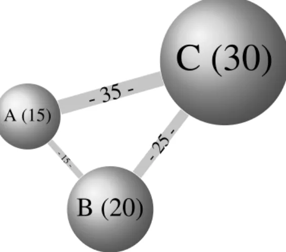
There are two key problems in NI dataset characterization: (1) Evaluation of the accuracy of the labels within the dataset and (2) Evaluation of how well the dataset represents the target traffic. Labeling has been addressed extensively in the literature, but there has been little focus on dataset representation . One study by Joseph et al. [28] proposed a unique validation method based on a community detection algorithm proposed by Schuetz et al. [46]. The algorithm is a very fast method of detecting the communities (groupings) among a network based on the difference between the number of connections between vertices and the number of connections which would exist between those vertices were the connections made randomly. The community detection algorithm results in a reasonable estimation of the communities extant within a network. Joseph et al. use the algorithm proposed by Schuetz et al. to produce a visualization of networks showing their communities. Multiple graphical entities are produced to allow visual analysis and comparison of datasets. Circles represent communities of hosts using particular protocols, where the diameter of the circle is proportional to the number of hosts within the community. Lines between the circles represent connections between hosts in the two communities, and the thickness of the line is proportional to the number of connections between the two communities. See Figure 2.1 for an example visualization, where the communities A, B, and C have 15, 20, and 30 hosts, respectively; and lines AB, BC, and AC consist of 15, 25, and 35 connections, respectively. Throughout the visual verification study, the supposition is that both dataset validation and verification of the topology and protocol distribution of multiple networks is being accomplished. However, the study does not specify which qualities of a dataset are being examined to determine the validity of each dataset. Examining the topological properties of
A (15)
B (20)
C (30)
- 15-- 35
--25-Figure 2.1: Example visualization of a small network consisting of three communities.
a network may be useful for general network traffic analysis, but defining which qualities of the topological properties will be used to validate one network against another is necessary if validation is the goal. The graphical visualization techniques and methods proposed in the visual verification study may be useful for traffic distribution analysis, as the visualization presented in the study is of traffic distribution and common protocol communities. The visual verification approach may also provide a view of how well a dataset consisting of generated traffic represents a particular network, but only in terms of protocol distribution and connections between communities. Joseph et al. acknowledge that their method is only useful to distinguish datasets with flawed topological and protocol distributions, and does not completely verify the quality of datasets. As proposed, the visual verification gives researchers a method of quickly viewing groupings within two networks to determine a rough estimate of their comparability. There is also a significant problem in using this method on collected traffic, as there is no verification of the traffic label accuracy. While the proposed visual verification method could be used as part of a general dataset validation methodology, alone it is unsuitable for quantitative NI dataset validation.
Other researchers have worked on accurately classifying packets into different categories to better understand the character of network traffic. Within the field of computer network traffic classification, there have been many studies on how to categorize network traffic, some of which are collected by Zhang et al. [62]. Focus has ranged from developing software to assist in the comparison of different NIAD classifiers on the same datasets [34] to an evaluation of the utility machine learning algorithms might have in network traffic classification [51]. All of these classification methods could be useful in determining overall patterns and distributions of network traffic. Identification of patterns and distributions would then be useful in developing models for generating background traffic to be used in NI datasets.
The severity of the labeling and representation accuracy problems depends on the type of dataset being created. If properly collected, datasets based on captured raw traffic can be assumed to be representative of the target network traffic [44]. However, the labels of a captured dataset are suspect, and lead to uncertainty for any studies using that dataset. Generated datasets, on the other hand, have accurate labels. However, there is currently no identified way to ensure that a given generated dataset is sufficiently representative of the target network traffic. As to hybrid methods of dataset creation, where there is a mix of captured live traffic and generated traffic, it is unknown whether the labeling and representation problems would be aggravated or diminished. One study by Mahoney and Chan [37] presented results suggesting that simulation artifacts in generated traffic can be eliminated by careful mixing of raw and generated traffic, but more work remains to generalize those results. As summarized in Table 2.1, this review has not discovered a method of dataset creation which results in both representative traffic and accurate labels.
Much research has been done on characterizing the IDEVAL [36] and derivative KDD99 [53] datasets. Critiques of the problems inherent in those datasets serve to highlight problems with generated datasets in general, and the methods used in their generation.
Table 2.1: Certainty of characterization of dataset creation methods
Certainty of Characterization
Dataset type Labels Representative
Captured Uncertain Certain
Generated Certain Uncertain
Hybrid Uncertain Uncertain
McHugh’s [38] analysis of IDEVAL resulted in recommendations including: The definition of metrics to measure performance, a calibrated and validated field-wide generated dataset or dataset generator, studies of false alarm rates in generated and collected datasets (to establish a relationship), research into creation of a field-wide set of network attack taxonomies, and a field-wide sharable source of recent attacks for use in research. Mahoney and Chan [37] performed a thorough examination of possible simulation artifacts within the IDEVAL datasets, and concluded that mixing real traffic with simulated traffic can remove those artifacts leading to a better evaluation of NIDS capabilities. Multiple studies of IDEVAL [16, 57] brought forth few new significant problems which generalize to simulated dataset generation not already noted, although they did conclude IDEVAL is still useful as a baseline for use in research.
NIAD research has been going on for many years. In spite of progress made in areas of NIAD research, including classification [30], anomaly detection [7], signature based detection [58], preprocessing [12], feature selection [8], and other topics; minimal work has been done on improving the pedigree of datasets used to validate NIAD classifiers. Many studies were performed with datasets local to the organization performing the research, or
originating from packet captures restricted from general use for legal reasons. With the different datasets used in performance evaluations over the years, it is difficult to accurately compare the results of one to another.
When characterizing datasets, there is implicit in the characterization the ability to compare one dataset to another. With the ability to compare one dataset to another, comes the concept of the difference between datasets and a quantifiable measure of that difference: the difference measure.
2.5 Difference Measures
There is a need to understand the current state of how distance measures are used in the field of NI. Knowledge of how the distance and similarity measures are used is insufficient, however, without knowledge of how well those measures used are identified by name or formula (or both) within the recently published papers. To provide a thorough overview, a recursive automated search is executed for the terms “network intrusion” in the title, abstract, or keywords using Google Scholar. The number of papers returned is limited by restricting the results to the first 100 returned papers, the depth of the reverse citation lookup to three, and the year published to between 2008 and 2012 (inclusive). The results provide the source for a random sample of the field.
There were 2,235 results returned by the search procedure. Due to time constraints a two pass method was used to eliminate papers. In the first pass, suitability for inclusion within the study is determined. Each paper is examined by hand and deemed unsuitable if it is a duplicate of a paper already examined, unrelated to the NID field, or unavailable electronically. Most of the papers are eliminated by that pass, leaving only 567. In the second pass, the remaining 567 papers are more closely examined to eliminate reviews, surveys, overviews, or examinations of the state of the art. The remaining 536 papers represent the most recent published papers in the field of NI.
As a full examination of all 536 papers is not possible within the time available, approximately 20% of the papers are randomly selected for inclusion in this sample. Each paper is examined to check for the following criteria.
1. The paper must contain results from classifying at least one NI dataset with the purpose of identifying attacks.
2. The paper must be available in English, or have an identification and formulation of distance measure use understandable regardless of the language.
The five papers that do not meet the two criteria above the number are discarded, leaving 100 papers. Each of those 100 papers is then examined to determine how (and if) the distance measures used within were named and formulated. For the full list of papers included in the survey, see Appendix A.
2.5.1 Evaluation of Measure Specificity.
As there sometimes exist differences in the terminology used to describe measures used, or between the formulation of each measure and those used in other works, this research uses the Encyclopedia of Distances [15] as the standard listing of measures. Any names and formulas found in the sample are compared to those within the Encyclopedia. It is useful to categorize the papers based upon explicit naming and formulation of distance measures used within the works, and the existence of those names and formulas within the Encyclopedia of Distances, effectively separating them into the categories ofGivenandNot given. However, it is apparent that some authors have developed new distance measures, or new names for existing distance measures, in response to the specific needs of the research being conducted. When the newly specified names and formulas are used, and are not identifiable in the Encyclopedia of Distances, an additional category is necessary: theNovelcategory.
To quantify how well the name and formulation of each distance measure matched the standard, a single set of categories are applied to the names and formulas used within each work, and a single definition of each category is used.
Among the works sampled for this review 60 of the papers did not provide a measure name, and 68 of the papers did not provide an explicit formulation. The sample taken indicates that most of the field does not provide names and formulas for the distance measures used within their research, and thus makes replication difficult. Ensuring clarity when specifying which and how each distance measure is used is critical to repeatability of published works. Vague descriptions and assumed measures lead to confusion at best, and incorrect implementations when attempting to duplicate experiments (thus incomparable results) at worst.
It is evident many different distance measures are used by researchers, but unfortunate how rarely they specify precisely which measures are used. One possible reason for the lack of specificity is the difference in terminology which exists among fields [15]. In example, if an author came to the AD field from the field of Ecology, or were familiar with the use of similarities in that field, they may use the term, “niche overlap similarity,” [43] instead of, “cosine similarity,” resulting in confusion to those unfamiliar with published works in the field of Ecology. An examination of the methods used by authors that do explicitly provide the name and formula of the measure(s) used, along with how clearly they explain the application of the measure and the phase in which it was used, is undertaken below.
2.5.2 Evaluation of Measure Types Used.
It is useful to understand which types of measures are being used in the field of NIAD, and which are not. When specifying the type of distance measure used, the names of types defined within the Encyclopedia of Distances are used: power (p,r)-distance, distances on distribution laws, and distances on strings and permutations. Disregarding the works without specified distance measures, there are 40 works within which distance measures are at least named, and three types of distances identified within the sampled works.
The first type of distance, the power (p,r)-distance, is shown in Equation (2.1). All instances of power (p,r)-distance observed within the sample used either the formula in Equation (2.1), or one that is mathematically equivalent.
The second and third types of distance used within the sample do not have a specific formula, as there is more variation among the implementations. The distribution of distance measures within the 40 papers is listed in Table 2.2.
Table 2.2: Frequency of difference measure types used within sampled works.
Measure type Number of papers
Power (p,r)-distance 22
Distances on distribution laws 15 Distances on strings and permutations 3
The majority of the distance measures used within the sample are based on the power (p,r)-distance and distances on distribution laws. Of the 22 uses of the power (p,r)-distance, 40% used Euclidean distance (p=r= 2). The sample shows that there is little exploration of the possible use of other measures within the field, as most of the measures are based upon the power (p,r)-distance or distances on distribution laws.
2.5.3 Distance Measure Categories.
In examining the types of distance measures used within the NI field, it is useful to consider distance measures as part of distinct families or categories. The families selected for this work are among those enumerated in, “Encyclopedia of Distances,” by Deza and Deza [15], where it is noted that the selection of a similarity index or distance measure is dependent in large part on the data. As there is no definitive taxonomy within the NID field, the measures and indexes examined will be ordered by their relationship to families of measures. As there are many published works in the NID field which do not identify
and specify the distance measures used, the focus in this section is to examine those papers which do both. This section provides examples of works in which the authors identify or formulate the measures used in a manner conducive to repetition or extension of their work. In particular, specificity when providing the formula for a distance or similarity measure is useful when repeating or extending works, and should be the standard rather than the exception. Unless otherwise noted below, the papers examined within this section provide good examples allowing duplication of the performed experiments by future researchers.
During this review it became evident that the three measure families most commonly used are those related to power (p,r)-distance, distances on distribution laws, and correlation similarities and distances. First, and most common, power (p,r) distance has already been defined in Section 2.5.2 and formulated in Equation (2.1). Second in popularity are distances on distribution laws, measures that apply to probability distributions over variables with the same range. Finally, correlation similarities and distances are measures that attempt to characterize the correlation between two datasets, and treat that as a measure of similarity or distance, rather than using the probability distributions or magnitude of vectors.
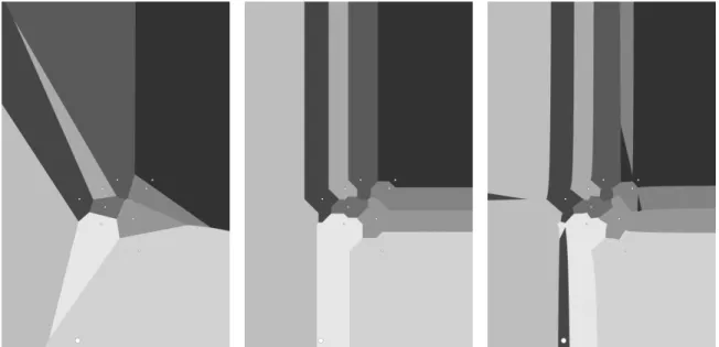
A large number of works within the NI field use power (p,r)-distance related distance measures. In particular many use Euclidean distance, which is an expression of Equation (2.1) where p=r =2. To provide some intuition about what different pandrvalues would mean when measuring the distance between two points, Figure 2.2 shows Voronoi diagrams [3] constructed using the power (p,r)-distance while varying the value of pandr.
After the measures related to power (p,r)-distance, those related to distances on distribution laws, or probability, were the next most common within the sample of the field (see Subsection 2.5.1) and literature review. While there is almost always an aspect of probabilistic behavior to any data collection and analysis, in this review the focus is on those studies which specifically used probability in one of the NID processes identified in Section 2.2.
Figure 2.2: Voronoi diagrams using power (p,r)-distance withp= r= h2,1,0.75i(from left to right).
One study in particular uses probability-related measures during feature selection. Hancock and Lamont [23] develop a, “Multi agent system for network attack classification using flow-based intrusion detection,” using the Bhattacharyya coefficient to rank features according to the ability of each feature to distinguish one class from the others. The Bhattacharyya coefficient is shown in Equation (2.3), where P1 and P2 are probability
distributions over the domainX,p1(x) is the probability ofxoccurring inP1, and p2(x) is
the probability ofxoccurring inP2.
ρ(P1,P2)=
X
x∈X
p
p1(x)p2(x) (2.3)
The three features with the largest overlap (largestρ(P1,P2) value) are selected after
rejecting any feature which is strongly correlated to a higher ranked feature to reduce redundancy among selected features. The feature selection is part of their second design iteration while pursuing the goal of an effective multi-agent NID system using reputation.
Hancock and Lamont identify the distance measure by name, but do not specify a formula with which to verify the work.
The least common measures used are those based on correlation similarities and distances. Zhao et al. [63] use a single distance measure which incorporates one of three correlation coefficients to detect stepping-stone attacks, where one computer is used by the attacker to reach another in, “Correlating TCP/IP Interactive Sessions with Correlation Coefficient to Detect Stepping-Stone Intrusion.”
The first correlation is the Spearman ρ rank correlation. Equation (2.4) gives the Spearmanρrank correlation whereXrandYrcontain the rankings of discrete variablesX and Y, xi and yi contain the ith rank in Xrand Yr (respectively), Xr and Yr have the same number of elements, andnis the number of elements inXr.
ρ(Xr,Yr)= 1− 6 n X i=1 (xi−yi)2 n(n2−1) (2.4)
The second correlation coefficient is similar to the Kendall τrank correlation. To properly define the Kendallτrank correlation a preliminary definition is required. Thesign, orsignum, function is defined in Equation (2.5).
sign(x)= −1, ifx< 0 0, ifx= 0 1, ifx> 0 (2.5)
The Kendall τ rank correlation can then be defined using the sign function as in Equation (2.6), where the signfunction is used to calculate the number of discordant pairs of ranks subtracted from the concordant pairs of ranks.
τ(Xr,Yr)= 2 n−1 X i=1 n X j=i+1 sign(xi− xj)·sign(yi−yj) n(n−1) (2.6)
The authors use an equivalent formulation, but to properly define the equivalent formula a preliminary definition of theequalsfunction is provided, as shown in Equation (2.7).
equals(x,y)= 1, x=y 0, otherwise (2.7)
The authors formulation ofτcan then be defined using theequalsandsignfunctions, and is shown in Equation (2.8).
τ(Xr,Yr)= 4 n−1 X i=1 n X j=i+1 equals(sign(xi− xj),sign(yi−yj)) n(n−1) −1 (2.8)
The third correlation coefficient is the Pearson product-moment correlation linear coefficient, orr. The formula forris given in Equation (2.9), where ¯X is the mean of the discrete variableX. r(X,Y)= n X i=1 xi−X¯ yi−Y¯ v t n X j=1 xi−X¯ 2 n X j=1 yi−Y¯ 2 (2.9)
The authors use an equivalent formulation, defined in Equation (2.10).
r(X,Y)= n n X i=1 xiyi− n X i=1 xi n X i=1 yi v u t n n X i=1 x2i − n X i=1 xi 2vut n n X i=1 y2i − n X i=1 yi 2 (2.10)
Each measure is applied to the two traffic streams, and each result is subtracted from one, to calculate the minimum distance between the two streams (σ(X,Y)), as shown in Equation (2.11).
σ(X,Y)= min(1−ρ(Xr,Yr),1−τ 0
(Xr,Yr),1−r(X,Y)) (2.11) If σ(X,Y) is less than a threshold set by the researcher, then the compared pair is relayed traffic. The use of multiple correlation coefficients within a single distance measure
is a good example of using multiple measures to detect similarities a single measure might not catch.
The predominant use of power (p,r)-distance and distances on distribution laws provides guidance on areas which have been explored in the current body of research. Also, the clear focus within the research on one or two measures per study is interesting, as it indicates further study of a multitude of measures applied to a single problem is, effectively, an open area.
Every experiment which utilizes AD in the NIAD field uses distance measures, most without much thought as to which distance measure would be most appropriate. Current research in the NIAD field is focused on the use of NIDS, rather than examining and characterizing NI datasets and the networks from which they are derived. However, the ways in which some distance and similarity measures are used can still be helpful in the comparison of datasets, as classifiers are, in some sense, distance measures: The accuracy of a specific classifier on a dataset, when compared with its accuracy on another, provides some knowledge of the difference between the two datasets.
The analysis and characterization of datasets which happens during the preprocessing, feature generation, and feature selection phases of NIDS is exactly what is needed when determining how to compare datasets. Using the knowledge, techniques and tools available in the NI field today, it should be possible to develop a methods to compare and characterize datasets without having to evaluate them using classifiers and feature selectors.
III. Methodology
The performance, or ability to successfully detect attacks, of a Network Intrusion Anomaly Detection (NIAD) classifier depends heavily on the characteristics of the network. The characteristics include the types of network traffic, frequency of attacks, and types of attacks on that network. Because classifier performance depends on those factors, and because those factors and classifier performance vary from network to network, there may be a correlation between classifier performance on two networks and the differences between those networks (provided the proper measure of difference can be found). In the NIAD field networks are commonly examined through logs of network traffic that are converted into datasets. As the focus of this work is on networks which are examined through datasets, within this worknetworkwill be used interchangeably withdataset. The hypothesis to be tested follows:
Hypothesis. The difference between two datasets, when calculated using the proper
difference measure, is correlated to the change in classifier performance between the two datasets.
To detect a correlation between the performance of a classifier on two datasets and the difference between the two datasets, there must be precise definitions of classifier
performanceand thedifferencebetween networks. While usually distance is used to denote a measured value representing the dissimilarity between two entities, distance is often interpreted as requiring non-negativity. For that reason, difference is used throughout this work to refer to the calculated measure of dissimilarity between two entities.
To measure classifier performance, three separate methods will be used. The first is the classifieraccuracy(A), which gives the overall ratio of correct classifications to number of
samples. To calculate the accuracy of the classifier Equation (3.1) may be used:
A= Pt+Nt Pa+Na
(3.1) wherePais the number of Actual Positives (AP) (total anomalous samples), Ptis the number of True Positives (TP) (correct anomalous classifications), Na is the number of Actual Negatives (AN) (total normal samples), andNt the number of True Negatives (TN) (correct normal classifications).
The second measure used is thetrue positive rateorsensitivity(RPt), which gives the proportion of correctly classified anomalous samples to the total number of anomalous samples. RPt can be calculated using the Equation (3.2):
RPt =
Pt
Pa
(3.2) The third measure used is thefalse positive rate(RPf), which provides the proportion of incorrectly classified normal samples to the total number of normal samples. To calculate
RPf, first the number of false positives must be calculated using Equation (3.3):
Pf = Na−Nt (3.3)
OncePf is known, thenRPf can be calculated using Equation (3.4):
RPf =
Pf
Na
(3.4) With a clear definition of classifierperformance, the focus can shift to defining what is meant by thedifferencewhen referring to datasets. Difference cannot initially be defined as clearly as performance, as a primary goal of this research is identifying one or more difference measures that properly characterize the difference between two networks and correlates well with the difference between classifier performance on the two networks. However, there are some characteristics of the difference between datasets that can be defined clearly. The following characteristics are useful qualities for a difference measure in this research.
• The difference measure must be a scalar, to provide a summary of dissimilarity which is also usable when developing a predictive model.
• The difference measure should provide both magnitude and sign, to adequately correspond to the sign of the change in accuracy.
In addition to defining a standard measure of difference between networks, identifying a difference measure which satisfies the above characteristics may be useful in predicting the performance of many kinds of classifiers on one network, based on the difference between that network and another.
3.1 Approach
To determine a suitable difference measure, identifying those elements of networks which have the greatest effect on classifier performance is key. NIAD classifiers depend on the separability of anomalous traffic, thus examining the ways traffic can be similar provides a useful starting point for difference measure selection. In general, the Anomaly Detection (AD) methods used in measuring differences between samples can be separated into two broad categories: spatial and probabilistic.
Spatial methods use the features of two samples as coordinates within the sample space, and compare the distance between two or more sets of samples to determine the difference between the samples. Those methods are then generalized to more than two samples, and used to measure the difference between two datasets. Probabilistic methods use the distribution of values within the features of a dataset, instead of the values themselves, to determine the overall probability distribution of the samples within the dataset. Measuring the difference between two datasets is accomplished by calculating the difference between the entropy of each dataset, using the probability distribution to calculate the entropy. As both methods can be useful in measuring difference, measures from both categories are used to measure difference in this work.
In developing experiments to test the Hypothesis 3, it is first useful to provide a structure that can be used to perform experiments. To do so, a System Under Test (SUT) is developed which represents the possible inputs, processes, and outputs involved in testing Hypothesis 3.
3.2 System Boundaries
The System Under Test (SUT) is the Classifier Accuracy Prediction System (CAPS) shown in Figure 3.1. The CAPS consists of an Anomaly Detection (AD) classifier, difference measure, correlation function to indicate if change in performance has a linear or rank-based correlation with the difference between the datasets, a linear model generator, and a predictive error calculator. Determination of how well a classifier performed on a given dataset is evaluated relative to how well it performed to another dataset. No attempt is made to determine which classifier is better, and feature generation and selection are not considered part of the test.
Classifier Accuracy Prediction System Anomaly Detection Classifier Difference measure Generator method Selector algorithm Difference measure Classifier Type Datasets (D) Linear Model Generator Prediction Error Calculator Quality of Prediction Correlator Correlation of difference measured to classifier performance change
The Component Under Test (CUT) is the difference measure. For identical datasets, upon which any classifier should perform identically, the difference measured should be statistically zero. For different datasets, the difference measured should be statistically non-zero.
3.3 System Services
The CAPS provides two services. The first is a set of values indicating how the difference measured among each pair of datasets correlates to the change in classifier performance between each corresponding pair of datasets. The difference is calculated using all difference measures. The second is the set of linear model prediction error values. To be considered successful, the difference measured between each pair of datasets must correlate consistently with classifier performance change between the same pair of datasets, and the linear models must be able to predict the changes in classifier accuracy based only on the differences measured between the datasets.
The CAPS takes as input a set of datasets (D). Each dataset is classified using an AD classifier. The difference (δ(i, j)) between every pair of datasets such thatndi,dj ∈D|i, j
o
is calculated. The change (ς(i, j)) in classifier performance between each pair of datasets is also calculated. The correlations of the set ofδ(i, j) andς(i, j) are calculated. The potential value of each correlation coefficient ranges from negative one to one. A zero means no significant correlation was found betweenδ(i, j) andς(i, j), whereas a negative one or one meansδ(i, j) andς(i, j) are perfectly correlated.
3.4 Workload
The workload consists of the datasets being compared by the CAPS, and the features included in each dataset. The features of the dataset are considered part of the workload parameters because they contain the values being considered when differences are calculated, therefore the correlation is based on these features.
3.4.1 Datasets.
In Network Intrusion Anomaly Detection (NIAD) research, there are two primary Network Intrusion (NI) datasets which have been used in the examination of AD classifiers: the 1999 Knowledge Discovery and Data Mining Tools Competition (KDD99) dataset [53] and the NSL-KDD [55] dataset. While those are ideal datasets to evaluate candidate difference measures once the candidates have been identified, time-constraints demand the use of less-complex datasets in the initial experiment.
The datasets used are a set of 38 2-D Synthetic Datasets [27], developed by Ji and Dasgupta [26]. They are designed to be used in AD classifier evaluation, and represent a variety of geometric shapes in different sizes as demonstrated by the visualization of one dataset in Figure 3.2. As the training datasets contain only self or non-self samples (depending on the perspective of the tester), only the test sets were used for this experiment.
0 0.2 0.4 0.6 0.8 1 0 0.2 0.4 0.6 0.8 1 x Normal data y 0 0.2 0.4 0.6 0.8 1 0 0.2 0.4 0.6 0.8 1 x Anomalous data y
Figure 3.2: The normal and anomalous data points inRing_midneg_testdataset. This is one of 38 synthetic datasets developed to test the abilities of AD classifiers.
As a result of using synthetic datasets of this type, there are limitations with regards to the claims that can be made based on the experimental results. First, the results may not be applicable to all datasets used within the NIAD field, but only to those which use datasets similar to those used in this study. Second, by using datasets designed with geometric shapes embedded within the data, there is an assumption made that datasets of interest will have shapes, and that the shapes will define the separation between anomalous and normal (non-self and self). That assumption may not be true for datasets commonly used in the NIAD field. Third, and finally, the synthetic datasets are two dimensional, whereas NI datasets can have tens or hundreds of dimensions. The results obtained here may not be applicable to datasets with higher dimensions.
Each of the datasets used consists of 1000 samples with two features: x and y
coordinates on a plane. Although it is common in the classification field to label anomalous and normal samples with a one and zero (respectively), the authors of these datasets labeled the anomalous and normal samples as zero and two (respectively).
3.5 Performance Metrics
The two primary performance metrics are the correlation coefficients used to determine the correlation between between the change in classifier performance and difference between datasets, and the quality of predictions by the linear models. The experiment is considered successful if there is consistent non-zero correlation between the dataset differences and corresponding changes in classifier performance,andif the prediction quality is non-zero.
The first performance metric is composed of two correlations. The first correlation is the Spearman rank correlation coefficient (ρ). The calculation ofρrequires the ranks of the data, not the values. The sign ofρ indicates the direction of association between the compared variables. The magnitude ofρindicates whether the value of the response variables (change inA,RPt, andRPf) are related monotonically to the predictor variable (difference between datasets). Given that xandycontain the rankings of the predictor and
response variables (respectively),Icontains the total number of values, andncontains the total number of ranks,ρcan be calculated using Equation (3.5):
ρ=1− 6 n(n2−1)
X
i∈I
(xi−yi)2 (3.5)
The second correlation is the Pearson product-moment correlation coefficient (r). The calculation ofrindicates the linear dependence of the two variables. Given that xand y
vectors that contain the values of the predictor and response variables (respectively), andn
contains the total number of values,rcan be calculated using Equation (3.6):
r= Pn i=1(xi−x¯)(yi−y¯) pPn i=1(xi− x¯)2pPni=1(yi −y¯)2 (3.6)
The second performance metric is the quality of the linear model predictions. The quality of prediction will be measured using the error between predicted and actual accuracies, or residuals, by examining the distribution of the residuals with respect to the distribution of the actual classifier performance values. Any ability to predict the actual performance values will be considered success.
In addition to the two checks for correlation and prediction quality, the results will be evaluated visually to ensure the results make sense. The first visual check is a series of scatter plots, using the predictor variable as the x-coordinate and the response variable as the y-coordinate.
The second visual check is a series of Quantile-Quantile (QQ) plots. A QQ plot is a probability plot which compares two probability distributions (histograms) using the same bins for each. The QQ plot is often used to compare a sample to a standard distribution, but instead it will be used to compared the distributions of differences and performance changes. Ideally, if they are from the same distribution they will align linearly along the diagonal.
3.6 System Parameters
3.6.1 Difference Measure.
The difference measured between two datasets (δ(i, j)) should determine how far apart two datasets are with respect to those characteristics which affect classifier performance. It affects the correlation significantly, and six different measures are used to quantify the difference between datasets.
The first five difference measures use entropy, as entropy gives an estimate of the predictability of the values in a dataset. The ability to calculate entropy requires the probability distribution of each feature (or each set of features), therefore the probability distribution must be calculated first. Calculating the probability distribution can be problematic in some datasets, because sometimes no value is repeated within a feature. As a result of that limitation, the probability distribution is estimated as follows. First, a reasonable bin-size is calculated using the Freedman-Diaconis rule [17].
h=2IQR(X)n−13 (3.7)
The function IQR(X) returns the interquartile range of the data in a feature vectorX, and nis the number of observations inX. Once the bin-size (h) is known, the set of bin edgeseare calculated:
l=min(X) u=max(X) b= & u−l h ' e=h−∞,l+h,l+2h, . . . ,l+(b−1)h,∞i (3.8)
Those calculations are performed for each feature. Once the edges are known, the values of each feature are sorted into bins while keeping count per bin. When complete the researcher is left with an estimate of the probability distribution of all features (p(F)). With
p(F), the entropy of each feature can be calculated using the standard formula for entropy:
H(X)= −X
x∈X
whereXis a feature inF (the set of all features).
The first difference measure is the difference between the sum of the entropy of each feature in two datasets. It is identified asδS, and is calculated between two datasetsdi and
djshown in Equation (3.10): δS = X X∈Fi H(X)− X Y∈Fj H(Y) (3.10)
where Fi and Fj are the set of features in datasets di and dj, respectively. The second difference measure is the absolute value of Equation (3.10). It is identified asδ|S|, and is shown in Equation (3.11).
δ|S| =|δS| (3.11)
The third difference measure is the sum of the absolute value of difference between the entropy of each feature. It is identified asδ|F|, and is calculated between two datasetsdiand
djas follows: δ|F| = X Xi∈Fi,Xj∈Fj H Xi −HYj (3.12)
whereFiandFj are the full set of features within datasetsdi anddj, respectively.
The fourth difference measure using entropy is the difference between the joint entropy
(H(Xs,Xt)) of two datasets. The joint entropy of a dataset with two features is calculated
using the joint probability distribution (p(X,Y)) of the features within the dataset:
H(X,Y)=−X
x∈X
X
y∈Y
p(x,y) log2(p(x,y)) (3.13) whereXandYare the two features within a dataset. A joint probability distribution can be calculated for more than two features:
H(X1,· · · ,Xt)=− X x1∈X1 · · ·X xt∈Xt p(x1,· · · ,xt) log2(p(x1,· · · ,xt)) (3.14)
whereXt is thetth feature in the dataset. This formulation is problematic in those datasets where all observations are unique in value, as it will result in maximal entropy, thus providing