Systematic feature analysis on timber defect images
Ummi Raba’ah Hashim a,1,*, Siti Zaiton Mohd Hashim b,2, Azah Kamilah Muda a,3, KasturiKanchymalay a,4, Intan Ermahani Abd Jalil a,5, Muhammad Hakim Othman c,6
a Computational Intelligence and Technologies Lab, Faculty of Information and Communication Technology,
Universiti Teknikal Malaysia Melaka (UTeM), Melaka, Malaysia
b Soft Computing Research Group, Faculty of Computing, Universiti Teknologi Malaysia (UTM), Johor, Malaysia c Faculty of Electronic and Computer Engineering, Universiti Teknikal Malaysia Melaka (UTeM), Melaka, Malaysia
1 [email protected], 2 [email protected], 3 [email protected], 4 [email protected], 5 [email protected], 6 [email protected]
* corresponding author
I. Introduction
Selecting the most significant features to distinguish between clear wood and defects remains a challenging issue to timber defect detection. There is a wide range of natural variations such as size, shape and tonal values across defects, and even between similar defect types. Moreover, grain appears to be unique across different timber species. In light of the timber defect detection issues, color or tonal values alone is not sufficient to describe the properties of a particular defect, for instance, knots can be as dim as pockets and some of them could have the same shading as clear wood [1]. Albeit most defects seem darker than clear wood, a defect can show up as dark as the wood grain itself sometimes. Hence, tonal properties alone are not adequate to describe timber defects [2]. Besides, since the samples used in our study are of different species, there will be variation in timber color. Accordingly, tonal measures are certainly not appropriate to represent defects crosswise over different timber species. Shapes and texture features are of equivalent significance to separate between clear wood and defects and also classes of defect [2]. But the inconsistency in the shape and size of defects minimises the practicality of using shape features in overcoming the timber defect detection problem. This is due to the difficulties in specifying an appropriate representation of various possible shapes of a defect.
While having no uniform surface, timber will generally have a unique pattern. The pattern describing timber appearance is called texture. Recognising and distinguishing this pattern with human vision is possible, however, characterizing the difference accurately is challenging. With a specific aim of introducing a species-independent timber defect detection system to overcome the tonal variation issues among timber species, utilization of texture features is proposed. Having known that texture is independent of tone [3], it is expected that it shall also be independent to timber species tonal variation. Since human vision is capable of distinguishing the texture difference between clear wood and defect, texture features are anticipated to work well in representing defects across timber
ARTICLE INFO A B S T R A C T
Article history:
Received July 27, 2017 Revised August 17,2017 Accepted August 17, 2017
Feature extraction is unquestionably an important process in a pattern recognition system. A clearly defined set of features makes the identification task more effective. This paper addresses the extraction and analysis of features based on statistical texture to characterize images of timber defects. A series of procedures including feature extraction and feature analysis was executed in order to construct an appropriate feature set that could significantly distinguish amongst defects and clear wood classes. The feature set is aimed for later use in a timber defect detection system. To assess the discrimination capability of the features extracted, visual exploratory analysis and statistical confirmatory analysis were performed on defect and clear wood images of Meranti (Shorea spp.) timber species. Findings from the analysis demonstrated that utilizing the proposed set of texture features resulted in significant distinction between defect classes and clear wood.
Copyright © 2017 International Journal of Advances in Intelligent Informatics. All rights reserved.
Keywords:
Texture Feature extraction Timber surface
Automated vision inspection Feature selection
species and defect types. Therefore, this study tries to examine the appropriateness of texture features for a future use in a timber defect detection system by looking at the capability of the texture features in discriminating between clear wood and defects.
This study investigates these wood texture features based on an orientation independent Grey Level Dependence Matrix (GLDM). The need to evaluate the performance of texture features on the timber defect detection task prompted the study, together with the promising performance of using GLDM for timber defect detection noted in previous studies [4]. According to a recent review of studies of vision inspection methods, statistical texture feature extraction is emerging as a popular method due to promising performance and the fact it can be applied directly without filtering [5]. Evolutions of the original GLDM, created by [3], include variations in the way in which the dependence matrix is generated and in the statistical features calculated from the matrix. It now has numerous applications across multiple domains.
II. Method
A. Overview of Approach
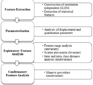
Fig. 1 illustrates the approach used to construct the significant feature set to characterize a timber defect. Firstly, an orientation independent GLDM is constructed and statistical features are extracted from the matrix at various quantization and displacement values. Secondly, multiple datasets are produced to analyze appropriate displacement and quantization parameters. The images, selected from the UTeM database [6], cover samples from eight defect classes and the clear wood class of Meranti timber species.
Thirdly, exploratory and confirmatory analyses are employed to further analyze the extracted features for their class discrimination capabilities. To visually examine discrimination between defect and clear wood classes, each of the following is used (i) a graph of feature range for each individual feature (univariate), (ii) a scatter plot matrix for pairwise features comparison (bivariate), and (iii) a graph of inter class and intra class distances for all features collectively (multivariate).
Finally, a confirmatory multivariate analysis of variance (MANOVA) statistically measures the class discrimination. Initially, features are tested for linear dependency using Pearson’s correlation coefficient and those with high linear dependency are eliminated and the remaining features are analyzed using MANOVA statistics. The ratio between inter class and intra class variances is then measured for the proposed feature set to confirm the significance of class discrimination, and thus yield a significant feature set.
B. Feature Extraction
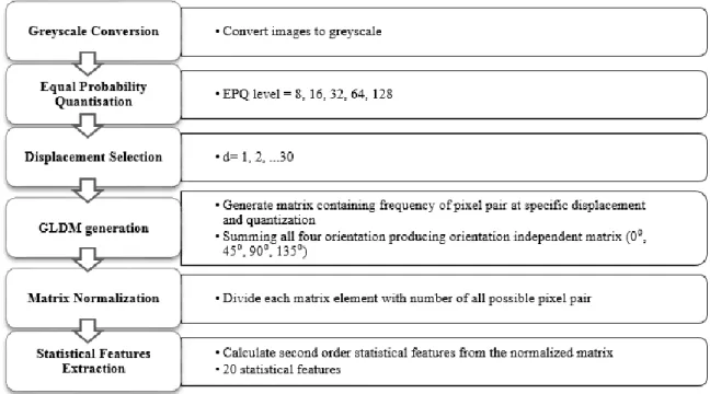
Fig. 2 shows the feature extraction process based on GLDM. The images were first converted to greyscale and, to reduce intensity levels of the images, equal probability quantization (EPQ) was employed. Equation (1) was then used to generate an orientation independent GLDM and the frequencies of pixel pairs at specific displacements for all considered orientations (0°, 45°, 90°, 135°) were added together [7].
𝐶(𝑘, 𝑙; 𝑑) ≡ ∑ 𝑖 ∑ 𝑗 ∑ 𝛿(𝑘 − 𝑔(𝑖, 𝑗))𝛿(𝑙 − 𝑔((𝑖, 𝑗) + 𝑑𝑛̂)) 𝑛̂ (1)
where n is the unit vector pointing in a chosen direction, g(i,j) is the intensity value of pixel (i,j), g((i,j)+dn) is the intensity value of neighbouring pixel at displacement d and orientation n and C(k,l;d) is the frequency of the pixel pair at displacement d, with k intensity value in one pixel and l intensity value in the other pixel. δ(a-b) takes value 1 if a=b and takes value 0 if a≠b.
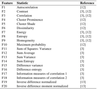
Features were iteratively extracted at several displacement and quantization values for further analysis of appropriate parameter selection. The matrix was then normalised by dividing each matrix element by the total frequency of pixel pairs in the matrix [8]. The resulting matrix is considered to be a joint probability density function from which statistical values can be calculated. As listed in Table 1, twenty statistical features were calculated from the resulting matrix.
Fig. 2. Procedures for extracting statistical texture features
Haralick et al. [3], on the assumption that all texture information is contained in the dependence matrix, proposed fourteen statistical formulas to characterize the texture presence in the original image. These formulas were extracted from the joint probability density function of the dependence matrix. Other researchers have since extended these formulations in various application domains to further represent the second order texture measure. These statistics measure the textural characteristics of the original image such as homogeneity, contrast, presence of structure, as well as the complexity and nature of tone transition [3]. Haralick et al. [3] claimed that it is difficult to specify the texture characteristics represented by each of the statistics. Using the statistics combined will give us the appropriate texture information represented in the image.
Recent work in this area closely related to wood defect detection involves detecting bark on logs [9]. According to Weidenhiller and Denzler [9], utilizing texture features derived from dependence matrices has produced promising results in bark detection. Findings of a defect classification study on plywood noted that features from a dependence matrix were useful in separating clear wood and defects [10]. Likewise, another recent study of hardwood and softwood using features from a dependence matrix reported good defect classification performance [11]. The similarities between the
work of Weidenhiller and Denzler [9] and our defect detection problem and given that both focus on wood products (logs and timber) which are, therefore, likely to be similar in appearance inspired us to investigate similar statistics to those employed in their study. However, our approach to generating the dependence matrix differed from their approach as our work considers many types of defects rather than bark detection only. Furthermore, we are working on tonal independent processing, hence, using GLDM instead of colour based matrix. In addition, we discovered some duplicate features in the extracted set, and thus these were removed from our study. The final list of second-order statistics (as shown in Table 1) was obtained via a combination of proposed features from multiple original references.
Table 1. List of Statistical Textures Features Extracted
Feature Statistic Reference
F1 Autocorrelation [12] F2 Contrast [3], [12] F3 Correlation [3], [12] F4 Cluster Prominence [12] F5 Cluster Shade [12] F6 Dissimilarity [12] F7 Energy [3], [12] F8 Entropy [3], [12] F9 Homogeneity [3], [12] F10 Maximum probability [12]
F11 Sum of Squares: Variance [3]
F12 Sum Average [3]
F13 Sum Variance [3]
F14 Sum Entropy [3]
F15 Difference variance [3]
F16 Difference entropy [3]
F17 Information measures of correlation 1 [3] F18 Information measures of correlation 2 [3] F19 Inverse difference normalized [13] F20 Inverse difference moment normalized [13]
III. Result of Analysis
A. Exploring Displacement and Quantisation Parameters of GLDM
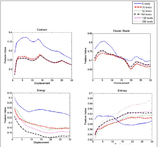
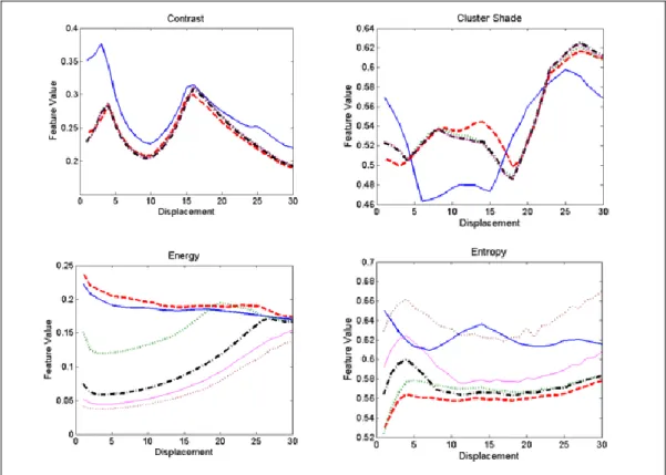
To determine the appropriate displacement and quantization parameters, feature extraction was repeated for 30 displacements and 5 quantization levels, Q=8, 16, 32, 64, 128, producing 150 datasets for analysis. In each dataset, the mean of the normalized features for each defect was calculated to better compare the feature values across quantization levels and displacement values. In this analysis, we used displacements, d=1,2,3…30. We used 30 as an upper limit as it is half of our image size (60x60). Fig. 3 and 4 shows a graph of normalized feature means against displacement and quantization values. For discussion purposes, the figure displayed only a few features: contrast, cluster shade, energy and entropy, for two defect classes, which are knots in fig. 3 and pocket in fig. 4.
In general, it can be observed that, the displacement curves were preserved nicely across different quantization levels for all features. The behavior of the curves is similar in terms of upward and downward slopes along the curves, indicating that the quantization level did not affect the texture properties. The difference is in the degree of the slopes which were probably caused by the reduced resolution when quantization levels were reduced. This indicates that although the loss of information was visible, the natural structure of the texture characteristics was still intact and can be represented by the GLDM. However, for some features, Q=8 and Q=16 noticeably deviated from other curves on a different range and some showed a dissimilar curve. Additionally, the graph for Q=8 was consistently and noticeably different from other levels for all feature graphs. Differences in curve and range indicate possible loss of information when the image was quantised to low resolution. For that reason, it is suggested that lower quantization values, Q=8,16 should not be used to avoid loss of texture information. For other quantization levels, however, the feature values were closely similar. Therefore, we can eliminate the need for higher quantization levels such as Q=64,128,256 which were computationally costly. Ma, Zhang, Wang, and Chen [14] supported that reduced quantization will
decrease computational load while not significantly affecting the discriminatory power of the GLDM. It is anticipated that successful classification can still be achieved even with a reduced quantization level. Hence, for further analysis, Q=32 was used as it represents similar texture information with higher quantization levels. Although the computational load for higher quantization values (Q=64,128,256) was high, they can still be used for the purpose of performance comparison in later analysis.
Looking at the displacement parameter, the graphs show a noticeable constant trend (upward or downward) up to a certain breakpoint where it started to show changes in slope degree or slope direction. This trend was clear for all features and the breakdown points were typically at d<5. This indicates that the texture property started to show structural changes as higher displacement values are used and at a certain displacement breakpoint, the matrix did not represent texture characteristics of the respective image. For that reason, we suggest that a displacement value of less than 5 (e.g. d=1) is appropriate to represent texture structure for our sample images. Additionally, several displacement values ranging from 1 to 3 can be used for comparison purpose in further analysis. This will provide confirmation on the most appropriate displacement value that allows us to capture the most texture information.
Fig. 4.Normalized feature means against displacement and quantization (Defect: Pocket) B. Exploratory Feature Analysis
1) Univariate Feature Range Analysis
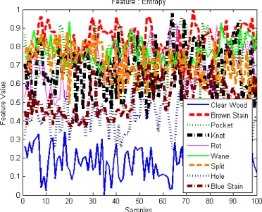
The purpose of feature range analysis is to analyze the discrimination between defect classes and the clear wood class for each feature. In this analysis, we selected 100 samples from each class and normalized the feature values. Then, the sample values were plotted on a graph to reveal the discriminative pattern of the classes accordingly for each feature. For discussion purposes, the graphs for only three features are displayed in Fig. 5, 6 and 7, which are energy, entropy and contrast. From the figures, we could see that defect classes were tightly clustered to each other while the clear wood class shows a clear distinction, deviating from other classes. This analysis revealed the usefulness of each feature in discriminating between defect and clear wood. Although it can be seen that the feature values between defect classes had similar ranges, they not really overlap or follow a similar trend. Thus, suggesting possible discrimination between defect classes as well.
Fig. 6.Entropy feature range analysis
Fig. 7.Contrast feature range analysis 2) Bivariate Matrix of Scatter Plot
The scatter plot matrix is used to visualize the discriminative pattern between classes, by comparing multiple features. However, the limitation of this plot is that it can only compare two features at a time. Additionally, the plot is more suitable for problems involving few classes only. If we have many classes, the plots will be too cluttered and will not be able to show us the patterns clearly. For that reason we used the scatter plot matrix to visualize the distinctive pattern between two classes: combined defects and clear wood. Fig. 8 shows the scatter plot matrix for three features as examples. As expected, the clear wood class was visually distinguishable from defect classes for all pairwise comparisons of features as depicted in Fig. 8, despite minor samples overlapping. In brief, it seems that the GLDM-based statistical texture features were able to measure the texture characteristics quite satisfactorily in terms of discriminating between clear wood and defect.
Fig. 8.Scatter plot matrix showing pairwise comparison of features 3) Multivariate Intra Class and Inter Class Distance between Clear Wood and Defect
In the previous analysis, we analyzed class discrimination for each individual feature (feature range analysis). Then, we analysed the class discrimination by pairwise comparison of features (scatter plot matrix). We further analysed class discrimination by taking into account all twenty features collectively using multivariate Mahalanobis distance. This analysis works by measuring the intra-class and inter-class distances using Mahalanobis formulation. The discriminative capability of features is made apparent by having a larger inter-class distance compared to intra-class distance.
For this analysis, we first calculated the mean and covariance of 50 independent clear wood samples. We then calculated the Mahalanobis distance between test samples and the obtained mean and covariance. The test samples comprised of 50 samples from each defect (eight defects) to calculate inter-class distance and 50 samples from the clear wood class to calculate intra-class distance. After that, we computed the mean distance for each class and finally plotted the graph as in Fig. 9. The figure shows the intra-class distance between clear wood samples (between test samples and independent samples) in red and inter-class distance between defect samples and independent clear wood samples in blue. It is obvious that the intra-class distance was much lower than the inter-class distance, indicating the discriminative power of the GLDM-based statistical texture features.
C. Confirmatory Feature Analysis
Confirmatory analysis is performed to measure class discrimination statistically using Manova procedures. In pre-Manova, features were tested for linear dependency (multicollinearity) using Pearson’s correlation coefficient where features with high linear dependency were removed from the feature set. Manova statistics were then computed based on the remaining features to measure the ratio between inter class and intra class variance.
The output of Manova statistics provided confirmation of the significance of the class discrimination, thus yielding a significant feature set. For confirmatory analysis using Manova, we used 100 samples per class. There are eight defect classes and one clear wood class, contributing to 900 samples.
1) Removing Linearly Dependent Features
Prior to calculating the Manova statistics, it is important to check for multicollinearity. Multicollinearity happens when features are linearly dependent, in other words, when one feature is a subscale or weighted average of the others. We performed correlation analysis between the features to test for multicollinearity. The correlation between features should be low to moderate for the Manova analysis to work best [13]. A strong correlation indicates redundant features (singularity), which decreases the efficiency of the Manova statistics. The original statistical texture features from the GLDM introduced by Haralick et al. [3] were claimed to be mostly correlated [14]. Therefore, to ensure the efficiency of the succeeding Manova statistics, we performed a Pearson’s correlation test to remove highly dependent features from our feature set (pre-Manova). In our study, if the correlation coefficient between features, r was higher than 0.99, the feature would be removed from the feature set.
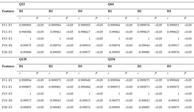
Table 2 shows the r value and the corresponding significance, P value for all features having r>0.99 across quantization levels, Q=32, 64, 128, 256 and displacements, d=1, 2, 3. Similar paired features were found to be linearly dependent, consistently across all quantization levels and displacement values. Table 3 listed the five features removed and the 15 remaining features.
Table 2. List of Feature Correlation with R>0.99
Features Q32 Q64 D1 D2 D3 D1 D2 D3 r P r P r P r P r P r P F11–F1 0.999995 <0.05 0.999994 <0.05 0.999955 <0.05 0.999994 <0.05 0.999976 <0.05 0.999951 <0.05 F13–F1 0.998586 <0.05 0.99961 <0.05 0.998617 <0.05 0.99961 <0.05 0.999615 <0.05 0.999622 <0.05 F15–F2 1 <0.05 1 <0.05 1 <0.05 1 <0.05 1 <0.05 1 <0.05 F19–F6 -0.99975 <0.05 -0.99974 <0.05 -0.99919 <0.05 -0.99974 <0.05 -0.99944 <0.05 -0.99917 <0.05 F20–F2 -0.99996 <0.05 -0.99995 <0.05 -0.99977 <0.05 -0.99995 <0.05 -0.99985 <0.05 -0.99976 <0.05 Features Q128 Q256 D1 D2 D3 D1 D2 D3 r P r P r P r P r P r P F11–F1 0.999994 <0.05 0.999975 <0.05 0.999949 <0.05 0.999994 <0.05 0.999975 <0.05 0.999949 <0.05 F13–F1 0.999897 <0.05 0.999901 <0.05 0.999904 <0.05 0.999972 <0.05 0.999973 <0.05 0.999972 <0.05 F15–F2 1 <0.05 1 <0.05 1 <0.05 1 <0.05 1 <0.05 1 <0.05 F19–F6 -0.99973 <0.05 -0.99943 <0.05 -0.99915 <0.05 -0.99973 <0.05 -0.99943 <0.05 -0.99915 <0.05 F20–F2 -0.99995 <0.05 -0.99985 <0.05 -0.99974 <0.05 -0.99995 <0.05 -0.99985 <0.05 -0.99975 <0.05
Table 3. List of Features Removed After Correlation Test
Feature Statistic Note
F1 Autocorrelation F2 Contrast F3 Correlation F4 Cluster Prominence F5 Cluster Shade F6 Dissimilarity F7 Energy F8 Entropy F9 Homogeneity F10 Maximum probability
F11 Sum of Squares: Variance Removed F12 Sum Average
F13 Sum Variance Removed
F14 Sum Entropy
F15 Difference variance Removed
F16 Difference entropy
F17 Information measures of correlation 1 F18 Information measures of correlation 2
F19 Inverse difference normalized Removed F20 Inverse difference moment normalized Removed
2) Measuring Significant Difference between Defect Classes using Manova Statistics
Prior to measuring the Manova statistics, we first tested the null hypothesis that the observed covariance matrices of the features are equal across classes using Box’s test of equality of covariance matrices (Box’s M). This test checks for the assumption of homogeneity of covariance across the classes with p<0.001 as a criterion. The result of this test determines which Manova statistics shall be used to interpret the subsequent result of class discrimination. From Table 4, Box’s M was significant, p(0.000)<α(0.001) indicating that there were significant differences between covariance matrices. Therefore, the assumption of homogeneity of covariance was violated. In this case, Pillai’s Trace is an appropriate test to use in interpreting our next Manova result as it is claimed to be robust to violation of homogeneity of covariance and not highly related to the assumption of normality of the data distribution [15].
A one-way Manova was conducted to test the hypothesis that there are no significant differences between classes. To test this hypothesis, a number of multivariate statistics can be calculated which are Wilk’s Lambda, Pillai’s Trace, Hotelling Trace and Roy’s Largest Root. Wilk’s Lambda is the most commonly used test when the assumption of homogeneity of covariance matrices is met. However, since we violated the assumption as discussed previously, we took a look at a test which is robust to the violation of this assumption which is Pillai’s Trace. From Table 5, we could see that the test result is significant, Pillai’s Trace=3.116, F(120,7072)=37.598, p<0.001. This indicates that there were significant differences between classes on the linear combination of all 15 features. In other words, the maximum ratio of between class variance to within class variance is significant, showing the usefulness of the feature set in discriminating defect classes as well as clear wood class.
Table 4. Box’s Test of Equality of Covariance Matrices
Variable Value Box’s M 17069.057 F 16.732 df1 960 df2 794123.202 Sig. .000
Table 5. Manova Test
Test Value Sig.
Pillai’s Trace 3.116 .000 Wilk’s Lambda .009 .000 Hotelling’s Trace 8.521 .000 Roy’s Largest Root 3.910 .000
Table 6 further shows the Pillai’s Trace value across multiple quantization levels and displacements. A higher Pillai’s Trace value denotes a higher ratio between class variance and within class variance. It is clear that the highest Pillai’s Trace value was shown in the dataset with Q=32 and d=1, indicating the highest class discrimination for this parameter set. It has been statistically confirmed that this parameter set is most suitable for our data. Therefore, in the future classification experiments, we shall use the dataset with Q=32 and d=1 to achieve maximum class discrimination, which is anticipated to lead to better detection performance.
Table 6. Pillai’s Trace Value across Multiple Quantisation Levels and Displacements
Quantisation Displacement Pillai’s Trace Sig.
Q32 D1 3.116 .000 D2 3.113 .000 D3 3.007 .000 Q64 D1 3.048 .000 D2 3.058 .000 D3 2.955 .000 Q128 D1 3.016 .000 D2 3.011 .000 D3 2.945 .000 Q256 D1 3.061 .000 D2 3.031 .000 D3 2.984 .000 IV. Conclusion
This study makes a number of important observations with respect to the representation of timber defects and clear wood using GLDM-based statistical texture features. For parameterization of the GLDM, analysis of displacement and quantization values was performed. Texture information was found to be consistent for low displacement values d<5 and higher quantization levels Q≥32, indicating no loss of texture information even when low resolution was used to generate the GLDM. To avoid excessive loss of texture information, using Q≥32 is suggested for our data. Depending on the hardware capability, the lowest quantization level recommended for our data is Q=32.
Visual exploratory analysis (univariate, bivariate, multivariate) suggested that all the features have appropriate class discrimination ability. However, when confirmatory statistical analysis was performed, some of the features were found to be linearly dependent, hence the respective features were removed. Manova statistics confirmed that there was significant difference between classes in the reduced feature set. This result is consistent over a range of displacement and quantization values (d=1,2,3; Q=32,64,128,256). However, the dataset with d=1 and Q=32 showed the highest ratio of inter class and intra class variance; hence, the most significant class discrimination.
The result of this study gives us an indication that the proposed features are sufficient to discriminate between defect classes as well as clear wood classes. Therefore, it can be emphasized that the quality of the proposed features is sufficient in terms of class discrimination capability especially between clear wood and defects, and therefore, appropriate to be further used in the next classification stage for solving the timber defect detection problem.
Acknowledgment
The researcher is sponsored by Ministry of Education, Malaysia and Universiti Teknikal Malaysia Melaka (UTeM).
References
[1] R. Conners, T. Cho, C. Ng, and T. Drayer, “A machine vision system forautomatically grading hardwood lumber,” Industrial Metrology, vol. 2, no. 1992, pp. 317–342, 1992.
[2] R. W. Conners, C. W. McMillin, K. Lin, and R. E. Vasquez-Espinosa, “Identifying and locating surface defects in wood: part of an automated lumber processing system.,” IEEE Transactions on Pattern Analysis and Machine Intelligence, vol. 5, no. 6, pp. 573–83, Jun. 1983.
[3] R. M. Haralick, K. Shanmugam, and I. Dinstein, “Textural Features for Image Classification,” IEEE Transactions on Systems, Man, and Cybernetics, vol. 3, no. 6, pp. 610–621, Nov. 1973.
[4] U. R. Hashim, S. Z. Hashim, and A. K. Muda, “Automated Vision Inspection of Timber Surface Defect: A Review,” Jurnal Teknologi, vol. 77, no. 20, pp. 127-135, 2015.
[5] X. Xie, “A Review of Recent Advances in Surface Defect Detection using Texture analysis Techniques,” Electronic Letters on Computer Vision and Image Analysis, vol. 7, no. 3, pp. 1–22, 2008.
[6] U. R. Hashim, S. Z. Hashim, and A. K. Muda, “Image Collection for Non-Segmenting Approach of Timber Surface Defect Detection,” International Journal of Advances in Soft Computing and its Application, vol. 7, no. 1, pp. 15–34, 2015.
[7] M. Petrou and P. G. Sevilla, Image Processing : Dealing with Texture. Wiley, 2006.
[8] U. R. Hashim, A. K. Muda, S. Z. Hashim, and M. B. Bonab, “Rotation Invariant Texture Feature based on Spatial Dependence Matrix for Timber Defect Detection,” in Intelligent Systems Design and Applications (ISDA), 2013 13th International Conference on, 2013, pp. 307–312.
[9] A. Weidenhiller and J. K. Denzler, “On the suitability of colour and texture analysis for detecting the presence of bark on a log,” Computers and Electronics in Agriculture, vol. 106, pp. 42–48, Aug. 2014. [10] G. A. Ruz, P. A. Estevez, and P. A. Ramirez, “Automated visual inspection system for wood defect
classification using computational intelligence techniques,” International Journal of Systems Science, vol. 40, no. 2, pp. 163–172, Feb. 2009.
[11] X. YongHua and W. Jin Cong, “Study on the identification of the wood surface defects based on texture features,” Optik - International Journal for Light and Electron Optics, 2015.
[12] L. K. Soh and C. Tsatsoulis, “Texture analysis of SAR sea ice imagery using gray level co-occurrence matrices,” IEEE Transactions on Geoscience and Remote Sensing, vol. 37, no. 2 I, pp. 780–795, 1999. [13] D. a. Clausi, “An analysis of co-occurrence texture statistics as a function of grey level quantization,”
Canadian Journal of Remote Sensing, vol. 28, no. 1, pp. 45–62, 2002.
[14] J. Ma, Z. Zhang, C. Wang, and Z. Chen, “Classifier-based feature fusion for texture discrimination,” in Proceedings of the 2009 International Conference on Information Engineering and Computer Science, ICIECS 2009, 2009.
[15] R. A. Horn, “Interpreting the One-way Manova,” Northern Arizona University, 2008. [Online]. Available: http://oak.ucc.nau.edu/rh232 /courses/EPS625/Handouts/InterpretingtheOne-wayMANOVA.pdf.