1
Serial Neural Network Classifier for Membrane
Detection using a Filter Bank.
Elizabeth Jurrus, Antonio R. C. Paiva, Shigeki Watanabe,
Ross Whitaker, Erik M. Jorgensen, and Tolga Tasdizen
UUSCI-2009-006
Scientific Computing and Imaging Institute
University of Utah
Salt Lake City, UT 84112 USA
June 30, 2009
Abstract:
Study of nervous systems via the connectome, i.e. the map connectivities of all neurons in that
sys-tem, is a challenging problem in neuroscience. Towards this goal, neurobiologists are acquiring large
electron microscopy datasets. Automated image analysis methods are required for reconstructing
the connectome from these very large image collections. Segmentation of neurons in these images,
an essential step of the reconstruction pipeline, is challenging because of noise, irregular shapes and
brightness, and the presence of confounding structures. The method described in this paper uses a
carefully designed set of filters and a series of artificial neural networks (ANNs) in an auto-context
architecture to detect neuron membranes. Employing auto-context means that several ANNs are
applied in series while allowing each ANN to use the classification context provided by the previous
network to improve detection accuracy. We use the responses to a set of filters as input to the
series of ANNs and show that the learned context does improve detection over traditional ANNs.
We also demonstrate advantages over previous membrane detection methods. The results are a
significant step towards an automated system for the reconstruction of the connectome.
Serial Neural Network Classifier for Membrane
Detection using a Filter Bank.
Elizabeth Jurrus
∗1,2, Antonio R. C. Paiva
1, Shigeki Watanabe
3,
Ross Whitaker
1,2, Erik M. Jorgensen
3, Tolga Tasdizen
4,11
Scientific Computing and Imaging Institute
2
School of Computing, University of Utah
3
Department of Biology, University of Utah
4
Department of Electrical Engineering, University of Utah
Abstract
Study of nervous systems via the connectome, i.e. the map connectivities of all neurons in that system, is a challenging problem in neuroscience. Towards this goal, neurobiologists are acquiring large electron microscopy datasets. Automated image analysis methods are required for reconstructing the connectome from these very large image collections. Segmentation of neurons in these images, an essen-tial step of the reconstruction pipeline, is challenging because of noise, irregular shapes and brightness, and the presence of confounding structures. The method described in this paper uses a carefully designed set of filters and a series of ar-tificial neural networks (ANNs) in an auto-context architecture to detect neuron membranes. Employing auto-context means that several ANNs are applied in se-ries while allowing each ANN to use the classification context provided by the previous network to improve detection accuracy. We use the responses to a set of filters as input to the series of ANNs and show that the learned context does improve detection over traditional ANNs. We also demonstrate advantages over previous membrane detection methods. The results are a significant step towards an automated system for the reconstruction of the connectome.
1
Introduction
Models of neural circuits are fundamental to the study of the central nervous system. However, relatively little is known about the connectivity of neurons, and many state-of-the-art models are insufficiently informed by anatomical ground truth. Electron microscopy (EM) is a particularly well suited modality since it provides the neces-sary detail for the reconstruction of large scale neural circuits, i.e., the connectome. However, the complexity and large number of images makes human interpretation an extremely labor intensive task. A number of researchers have undertaken extensive EM
. . . NN2 NNn NN1 I C T F S
Figure 1: Serial neural network. I: Input, F: filter bank, S: neighborhood stencil, C: context image, T: threshold.
imaging projects in order to create detailed maps of neuronal structure and connectiv-ity [12, 3, 2]. A significant portion of neural circuit reconstruction research has focused on the nematode C. elegans which has only 302 neurons and is one of the simplest or-ganisms with a nervous system. In spite of its simplicity, the manual reconstruction effort is estimated to have taken more than a decade. Newer imaging techniques are providing even larger volumes from more complex organisms, further complicating the circuit reconstruction process [1]. There is a need for algorithms that are sufficiently robust for segmenting neurons with little or no user intervention.
Segmentation of neurons from EM is a difficult task. The quality and noise in the image can vary depending on the thickness of the EM sections causing the membranes to change in intensity and contrast. In addition, intracellular structures such as mi-tochondria and synaptic vesicles render intensity thresholding methods ineffective for isolating cell membranes (Figure 4(b)). The method described in this paper uses a se-ries of artificial neural networks (ANNs) to more accurately detect membranes in EM images, which is a necessary step for improved three-dimensional neuron segmenta-tion. The first ANN uses as input a bank of oriented filters that were designed to match membranes. The input to the subsequent ANNs in the series is the same set of filters responses, in addition to the output of the previous ANN on a stencil of nearby pixels (as depicted in Figure 1). The idea is that ANNs along the series are able to conciliate context information about likely classifications of pixels across the image.
2
Background
There are several methods that attempt to segment EM images of neural tissue. Simple thresholding methods can be applied after isotropic or anisotropic smoothing [10, 6], but these fail to remove internal cellular structures and simultaneously detect a suffi-ciently high percentage of the true membranes to make accurate segmentations. While active contours, in both parametric and level set forms [5, 7], can provide smooth, accurate segmentations, they require an initialization and are more appropriate for seg-menting a few cells. If the goal is the automatic segmentation of hundreds or thousands of cells, manual initialization is not practical, and an automatic initialization is as diffi-cult as isolating the individual cells—which is the purpose of this work.
In related work, Jain et al. used a multilayer convolutional ANN to classify pixels as membrane or non-membrane in specimens prepared with an extracellular stain [4]. This stain however greatly increases the contrast between the cell boundaries and intra-cellular structures, and therefore significantly simplifies the segmentation task. On the
Figure 2: Stencil neighborhood of size11×11pixels is used on the output of each
ANN to gather context on the output of the ANN.
other hand, neural circuit reconstruction also requires the detection of synapses, which is only directly possible when intracellular structures are observed and thus cannot be obtained through the previous approach. Furthermore, the ANN approach by Jain et
al. contains more than 30,000 parameters and, therefore, is computationally intensive
and requires very large training sets. On the other extreme, even a perceptron applied to a carefully chosen set of features has been shown to provide reasonable results in identifying membranes in EM images [8]. Nevertheless, this method still requires sig-nificant post processing to connect membranes and remove internal cellular structures. In Jurrus et al. [6], a contrast enhancing filter followed by a directional diffusion filter is applied to the raw images to enhance and connect cellular membranes. The images are then thresholded and neuron membranes are identified using a watershed segmenta-tion method. An optimal path computasegmenta-tion is performed to join segments across slices, resulting in a segmentation in three dimensions.
Of conceptual relevance to this work is Tu’s auto-context method [11], which uses a series of classifiers utilizing contextual inputs to classify pixels in images. In Tu’s method, the “continuous” output of a classifier, considered as a probability map, and the original set of features are used as inputs to the next classifier. The probability map values from the previous classifiers provide context for the classifier, by using a feature set that consists of samples of the probability map at a large neighborhood around each pixel. Each subsequent classifier extends the influence of the probability map in a nonlinear way, and thus the system can learn the context, or shapes, associated with a pixel classification problem. Theoretically, the series of classifiers improves an approximation of a posteriori distribution [11].
3
Method
The method for membrane segmentation developed here combines the responses from a filter bank designed to match membranes with a series of ANNs for auto-context [11]. Auto-context learns from image features computed at local pixels and a classification map applied to the classifier output. The classification map is a stencil placed over each pixel containing information about the features in surrounding pixels, that is not rep-resented in the original feature set (Figure 2). This allows the networks at subsequent steps of the series, show in Figure 1, to make decisions about the membrane classifica-tion utilizing nonlocal informaclassifica-tion. Put differently, each stage in the series accounts for
(a) (b) (c)
Figure 3: (a) Membrane, (b) junction, and (c) vesicle detection filters used for input into the neural network.
larger structures in the data, taking advantage of results from all the previous networks. The advantages of this architecture are shown later for closing of weak membranes and removal of intracellular structures after each iteration in the series. Combining the orig-inal filter responses with features from the output of the classifier is important because, in this way, the relevant membrane structure for segmentation is enforced locally and then again at a higher level from each step in the series of classifiers.
Given the success of ANNs for membrane detection [8, 4] and because auto-context is not specifically tied to any classifier, we implement a multilayer perceptron (MLP) ANN as our base classifier. An MLP is a feed-forward network which approximates a boundary with the use of ridges given by the nonlinearity at each node. In our case, each network has one hidden layer with 20 nodes. Although we experimented with the use of two hidden layers, no advantage was observed. The output of each node is given
as,y=f(wTx+b), wheref is in our case the tanh nonlinearity,xdenotes the inputs,
wis the weight vector, andbis a bias term. The inputs to the first network include the
image intensity and the response to a bank of feature detection filters, described next. The image features the first ANN uses to learn are membrane and vesicle detection filters. We chose to use filters to detect features and train the network rather than learning the filters because we have prior knowledge about the membrane geometry and can design a match filter to detect them. Three types of feature detection filters were constructed to generate responses for the different types of membranes (see Figure 3). The first and second filter types are both bars, one to detect membranes and the other to detect membrane junctions. The width of the bar approximates the width of the membrane, which in our case is about 5-7 pixels wide. To detect membranes at different
angles, each filter is rotated between 0 and 180 by20◦. The third filter type is a simple
vesicle detection filter which helps the network learn pixels it should not classify as membranes, i.e., for rejecting vesicles. It is constructed as a circle with an off center surround ranging in radius depending on the size of the vesicles in the images. For the data utilized, the radius varies between 3 and 5 pixels. Each filter is convolved with
each pixel in the image:Ii =I∗Fi, whereIis the input image andFiis theith filter
convolved withI. The complete filter bank,F, contains the membrane and junction
filters, at rotational increments of20◦, and several scales of vesicle filters, for a total of
32 filters.
Using principles from auto-context, we implemented a serial classifier that lever-ages the output of the previous network to gain knowledge of a large neighborhood. For the first classifier, the input is the set of outputs from the filter bank. For the remaining steps, data from the stencil is gathered from the output of the previous classifier,
rein-forcing the membrane structure from one classifier to the next. The input is then the output of the stencil applied to the context image, and the set of filters in the original image. Figure 1 demonstrates this flow of data between classifiers. Each ANN
pro-duces a classification, or context image, denotedC, and the final output is thresholded
inT after the last ANN in the series.
By using a filter bank as the initial input, the network can quickly learn the context of the data it is trying to classify, while also acting as a regularization term for the learning algorithm. It better represents the type of data being learned. With each step in our serial classifier, context allows the network to use information about structure from a broader image neighborhood to the pixel being classified, while the filters inputs reinforce the elongated structure of membranes. This results in segmentations that im-prove after each network in the series. Figure 5 visually demonstrates the classification improving between ANNs in the series. Much like a convolutional network, at each stage of the series, the network uses more context around each pixel to make a clas-sification. This means that learning and application of the classifier is more efficient since one does not have to deal with large image features, and the network does not have the task of inferring the elementary structure from the dataset, i.e., find the filters. Consequently, this accounts for a smaller and simpler network which can be trained from smaller datasets. Overall, our implementation also has advantages due to the use of multiple networks. This approach provides better control of the training, allowing the network to learn in steps, refining the classification at each step as the context in-formation it needs to correctly segment the image increases. Hence, our approach is much more attractive to train, as opposed to utilizing a single large network with many hidden layers and nodes. Using a single large network would be time consuming and difficult to train due to the many local minima in the performance surface, and requires large training datasets which are hard to obtain since the ground truth must be hand labeled.
4
Results
The ANNs used in our tests are solved with backpropagation using a step size of.0001
and a momentum term of.5. To avoid local minima in computing the best set of weights
at each series in the network, the ANN uses cross-validation and Monte Carlo simula-tions. The network is trained using cross-validation on a portion of the input data, and the network terminates when the cross-validation error increases for 3 consecutive iter-ations. To compute the best set of weights, 10 Monte Carlo simulations of the network are run, each with a different set of random weights. The weights from the network with the highest percentage of correctly trained instances in the cross-validation set are used to compute the segmentation for that step in the series. The time it takes to train 1 ANN is approximately 3-6 hours.
An expert classified 50 images in the dataset, carefully marking membranes. The negative training examples are the remaining pixels in the image, after morphological erosion to remove training pixels that are very close to the membranes. This ensures that the network learns on pixels that are membrane and non-membrane, but does not become confused by pixels that are neither.
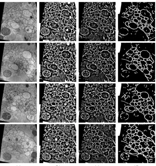
(a) (b) (c) (d)
Figure 4: Different membrane segmentations for four test images, each trained using one fold from the five fold cross-validation strategy. (a) Cross-section of the nematode
C. elegans with a resolution of 6nm×6nm×33nm, acquired using EM. Three demon-strated segmentation techniques: (b) thresholding on the CLAHE enhanced, smoothed data, (c) thresholded boundary confidences using Hessian eigenvalues, and (d) the pro-posed method, serial ANNs, trained using membrane filter banks and auto-context.
(1) (2) (3) (4)
Figure 5: An example of an image in each stage (1-4) of the network series. At each stage, the network learns more about pixels that do and do not belong to the mem-brane. The top row is the output from the neural network, and the bottom row is the thresholded output.
To test the robustness of the method, we use five fold cross-validation on the set of 50 C. elegans expert annotated EM images. The 50 images are separated into groups of 10. For each fold, the network is trained on one group and tested on the remaining four groups. The only preprocessing performed for each image is a contrast limited adaptive histogram equalization (CLAHE) [9] filter, with a window size of 64, to en-hance the contrast of the membranes before the filter bank is applied. Figure 4 shows a set of test images along with the segmentation found using different methods. The first method, shown in the 2nd column, performs thresholding after the contrast is enhanced and anisotropic smoothing is performed. The 3rd column is a segmentation similar to Mishchenko [8], who learns boundary confidences using Hessian eigenvalues as input to a single layer neural network. Mishchenko performs further post-processing to in-terpolate between broken boundaries and complete contours, resulting in an improved segmentation compared to the one shown here. We compare against only the single layer network part of his method since our goal is to demonstrate the improvement achieved by the use of an ANN and auto-context. Furthermore, the same preprocessing methods could be applied to the results of the proposed method as well. The final col-umn is the segmentation found using the serial network presented in this paper. For this particular data set, we chose a network series that consists of 5 ANNs. Figure 5 shows the output between each network in the series. At each stage, the network removes internal structures and closes membrane gaps. Over several networks, this results in noticeable improvements in the membrane segmentation.
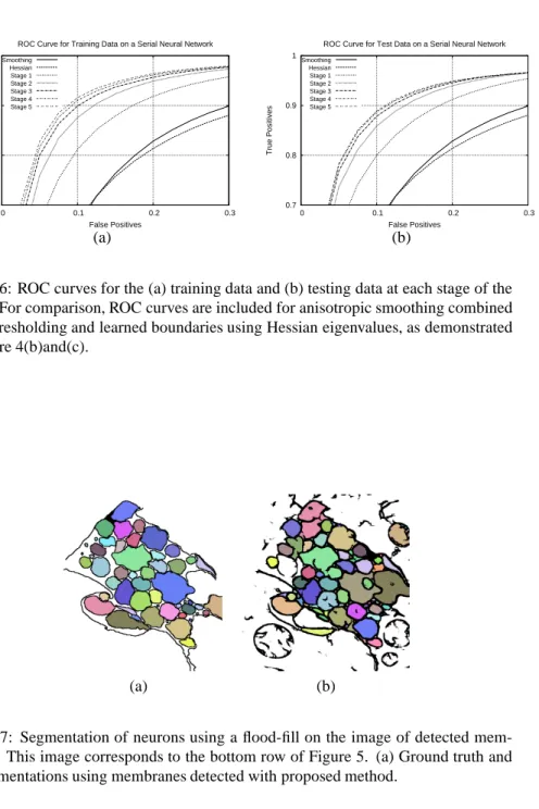
The receiver operating characteristic (ROC) curves in Figures 6 demonstrate the improvement in the segmentation at each stage of the series. Each curve is computed by averaging, for the stage, the ROC curves over all cross-validation folds. Even after just one stage of the network, the classification has improved dramatically. Further stages help to refine the membrane locations and remove structures remaining inside the membranes.
It is important to compare the final neuron segmentation that the different methods produce. Figure 7 demonstrates the differences between the segmentations using the
0.7 0.8 0.9 1 0 0.1 0.2 0.3 True Positives False Positives
ROC Curve for Training Data on a Serial Neural Network Smoothing Hessian Stage 1 Stage 2 Stage 3 Stage 4 Stage 5 0.7 0.8 0.9 1 0 0.1 0.2 0.3 True Positives False Positives
ROC Curve for Test Data on a Serial Neural Network Smoothing Hessian Stage 1 Stage 2 Stage 3 Stage 4 Stage 5 (a) (b)
Figure 6: ROC curves for the (a) training data and (b) testing data at each stage of the series. For comparison, ROC curves are included for anisotropic smoothing combined with thresholding and learned boundaries using Hessian eigenvalues, as demonstrated in Figure 4(b)and(c).
(a) (b)
Figure 7: Segmentation of neurons using a flood-fill on the image of detected mem-branes. This image corresponds to the bottom row of Figure 5. (a) Ground truth and (b) segmentations using membranes detected with proposed method.
proposed method. While this segmentation is not perfect, it is a large improvement upon previous methods. For a complete segmentation to be possible, minor hand edits are required along with some region closing techniques to be considered as future work.
5
Conclusion and Future Work
In this paper we propose the combined use of filter banks, principles from auto-context, and a series of ANNs for the segmentation of neuron membranes in EM images. On one hand, the application of filters to the input data and a stencil to the output of each classifier gives context for the classifier to use to close gaps in membranes and remove internal structures. On the other hand, both the filters and serial ANN architecture in the framework act as regularization terms, forcing the network to learn incrementally, using features that match the data on at multiples context scales provided by each step. In spite of the specificity of this application, the concepts and framework proposed may be potential useful in other domains. For example, similar strategies could also prove successful in segmenting long tubular structures such as vasculature in MRI, due to the capability of closing gaps in weak areas of elongated structures.
Acknowledgements
This work was supported by NIH R01 EB005832 (TT), HHMI (EMJ), and NIH NINDS 5R37NS34307-15 (EMJ).
References
[1] J. Anderson, B. Jones, J.-H. Yang, M. Shaw, C. Watt, P. K. abd J. Spaltenstein, E. Jur-rus, K. U. V, R. Whitaker, D. Mastronarde, T. Tasdizen, and R. Marc. A computational framework for ultrastructural mapping of neural circuitry. to appear PLoS, 2009. [2] K. L. Briggman and W. Denk. Towards neural circuit reconstruction with volume electron
microscopy techniques. Current Opinion in Neurobiology, 16(5):562–570, October 2006. [3] J. C. Fiala and K. M. Harris. Extending unbiased stereology of brain ultrastructure to
three-dimensional volumes. J Am Med Inform Assoc., 8(1):1–16, 2001.
[4] V. Jain, J. Murray, F. Roth, S. Turaga, V. Zhigulin, K. Briggman, M. Helmstaedter, W. Denk, and H. Seung. Supervised learning of image restoration with convolutional net-works. IEEE 11th International Conference on Computer Vision, pages 1–8, Oct. 2007. [5] E. Jurrus, M. Hardy, T. Tasdizen, P. Fletcher, P. Koshevoy, C.-B. Chien, W. Denk, and
R. Whitaker. Axon tracking in serial block-face scanning electron microscopy. Medical
Image Analysis, 13(1):180–188, Feb 2009.
[6] E. Jurrus, R. Whitaker, B. Jones, R. Marc, and T. Tasdizen. An optimal-path approach for neural circuit reconstruction. In Proceedings of the 5th IEEE International Symposium on
Biomedical Imaging: From Nano to Macro, pages 1609–1612, 2008.
[7] J. Macke, N. Maack, R. Gupta, W. Denk, B. Sch¨olkopf, and A. Borst. Contour-propagation algorithms for semi-automated reconstruction of neural processes. J Neurosci Methods, 167:349–357, 2008.
[8] Y. Mishchenko. Automation of 3d reconstruction of neural tissue from large volume of conventional serial section transmission electron micrographs. J Neurosci Methods, Sept 2008.
[9] S. Pizer, R. Johnston, J. Ericksen, B. Yankaskas, and K. Muller. Contrast-limited adaptive histogram equalization: speed and effectiveness. Visualization in Biomedical Computing,
1990., Proceedings of the First Conference on, pages 337–345, May 1990.
[10] T. Tasdizen, R. Whitaker, R. Marc, and B. Jones. Enhancement of cell boundaries in transmission electron microscopy images. In ICIP, pages 642–645, 2005.
[11] Z. Tu. Auto-context and its application to high-level vision tasks. Computer Vision and
Pattern Recognition, IEEE Conference on, pages 1–8, June 2008.
[12] J. White, E. Southgate, J. Thomson, and F. Brenner. The structure of the nervous system of the nematode caenorhabditis elegans. Phil. Trans. Roy. Soc. London Ser. B Biol. Sci., 314:1–340, 1986.