CEC Theses and Dissertations College of Engineering and Computing
2016
Using Diversity Ensembles with Time Limits to
Handle Concept Drift
Robert M. Van Camp
Nova Southeastern University,[email protected]
This document is a product of extensive research conducted at the Nova Southeastern UniversityCollege of Engineering and Computing. For more information on research and degree programs at the NSU College of Engineering and Computing, please clickhere.
Follow this and additional works at:https://nsuworks.nova.edu/gscis_etd
Part of theComputer Sciences Commons
Share Feedback About This Item
This Dissertation is brought to you by the College of Engineering and Computing at NSUWorks. It has been accepted for inclusion in CEC Theses and Dissertations by an authorized administrator of NSUWorks. For more information, please [email protected].
NSUWorks Citation
Robert M. Van Camp. 2016.Using Diversity Ensembles with Time Limits to Handle Concept Drift.Doctoral dissertation. Nova Southeastern University. Retrieved from NSUWorks, College of Engineering and Computing. (984)
Using Diversity Ensembles with Time Limits to Handle Concept Drift
by
Robert Van Camp
A dissertation report submitted in partial fulfillment of the requirements for the degree of Doctor of Philosophy
in
Computer Information Systems
Graduate School of Computer and Information Sciences Nova Southeastern University
We hereby certify that this dissertation, submitted by Robert Van Camp, conforms to acceptable standards and is fully adequate in scope and quality to fulfill the dissertation requirements for the degree of Doctor of Philosophy.
_____________________________________________ ________________
Sumitra Mukherjee, Ph.D Date
Chairperson of Dissertation Committee
_____________________________________________ ________________
Michael J. Laszlo, Ph.D. Date
Dissertation Committee Member
_____________________________________________ ________________
Francisco J. Mitropoulos, Ph.D. Date
Dissertation Committee Member
Approved:
_____________________________________________ ________________
Yong X. Tao, Ph.D., P.E., FASME Date
Dean, College of Engineering and Computing
College of Engineering and Computing Nova Southeastern University
An Abstract of a Dissertation Report Submitted to Nova Southeastern University in Partial Fulfillment of the Requirements for the Degree of Doctor
of Philosophy
Using Diversity Ensembles with Time Limits to Handle Concept Drift
by
Robert Van Camp 2016
While traditional supervised learning focuses on static datasets, an increasing amount of data comes in the form of streams, where data is continuous and typically processed only once. A common problem with data streams is that the underlying concept we are trying to learn can be constantly evolving. This concept drift has been of interest to researchers the last few years and there is a need for improved machine learning algorithms that are capable of dealing with concept drifts. A promising approach involves using an ensemble of a diverse set of classifiers. The constituent classifiers are re-trained when a concept drift is detected. Decisions regarding the number of classifiers to maintain and the frequency of re-training classifiers are critical factors that determine classification accuracy in the presence of concept drift. This dissertation systematically investigated these issues in order to develop an improved classifier for online ensemble learning. The impact of reducing the time requiring additional ensembles was studied using artificial and real world datasets. Findings from these studies revealed that in many cases the number of time steps additional ensembles are in memory can be reduced without sacrificing prequential accuracy. It was also found that this new ensemble approach performed well in the presence of false concept drift.
Acknowledgements
Completing my dissertation has been a rewarding personal experience for me. I believe going through this process will help me as I work with my students in the future. First, I would like to thank my advisor, Dr. Sumitra Mukherjee, for serving as my dissertation chair. Dr. Mukherjee consistently encouraged me along this path, from problem
definition to dissertation defense. I greatly appreciate his help. In addition, my thanks to Dr. Michael Laszlo and Dr. Francisco Mitropoulos for their willingness to serve on my committee and provide valuable feedback.
Dr. Leandro Minku was gracious enough to provide the C code used for the original DDD algorithm. I appreciate his willingness to do so.
I would like to thank Marietta College for providing support for travel and for a
sabbatical to aid in completing my dissertation. I would like to thank Dr. John Tynan and Dr. Mark Miller, my current and previous department chairs, for encouraging me in this process. I would like to thank my colleagues at Marietta College for words of support, especially those in my department.
I would also like to thank my children, Bethany Richetti and Will Van Camp, for their belief in me during these last six years. I wish the best for them in their studies. I also thank the rest of my extended family, including my mother-in-law Retta Wayne, who always asked how I was getting along with my research. My father-in-law, Wilson Wayne, is no longer here but was always a source of encouragement. While they are no longer here, I thank my father and mother, Don and Ruth Van Camp, they instilled in me a belief I could succeed in whatever I put my mind to. I know they would be happy and proud.
Finally, I would like to thank my wife, Mary Ellen. She has been my constant supporter in this dissertation process. She has been my proofreader, sounding board, and best friend. I could not have completed this dissertation process without her love and encouragement.
Table of Contents Abstract ii
List of Tables viii
List of Figures ix List of Algorithms xi Chapters 1. Introduction 1 Background 1 Problem Statement 8 Dissertation Goal 9
Relevance and Significance 9 Barriers and Issues 10
Assumptions, Limitations, and Delimitations 10 Summary 11
Definition of Terms 12
2. Review of the Literature 15
Overview 15
Justification of Review Criteria 15 Types of Machine Learning 16
Strategies for Supervised Learning 16 Definition of Concept Drift 17
Highlights in Concept Drift Research 19 Ensemble Methods with Concept Drift 19 Concept Drift Detection 20
EDDM 21 DWM 23
Diversity with Ensembles 24 DDD Algorithm 26
False Positives in Concept Drift 27
Comparison of EDDM, DWM, and DDD 27 Performance Evaluation 28
Summary 29
3. Methodology 31
Overview of Methodology 31 Maximum Time Step Parameter 32 Testing with Artificial Datasets 32 Testing with Real World Data 36
Comparison with other Concept Drift Algorithms 38 Testing for False Positive Concept Drift 38
Preliminary Work 39 Detailed Test Plan 42 Resources Used 44 Summary 44
4. Results 45
Introduction 45
Determine Best MTS 46
Results of Comparison with other Concept Drift Algorithms 61 Results of Tests for False Positive Concept Drift 77
Summary of Results 91
5. Conclusions, Recommendations, and Summary 92
Conclusions 92 Recommendations 93 Summary 94
Appendices 96
Appendix A – Comparison of Various MTS Settings 96 Appendix B – Frequency of MTS Values 105
Appendix C – Comparison of Best MTS, DDD, and DDD with Reset 107
Appendix D – Best MTS and Standard DDD, Average Time Steps in Four Ensembles 116 Appendix E – Comparison of Various W Settings using Best MTS 123
Appendix F – Comparison of Various W Settings using Standard DDD 132
References 141
List of Tables
Tables
1. Examples of Severity 8 2. Definition of Terms 12
3. Severity for Artificial Datasets 34 4. Settings for Artificial Datasets 36 5. Settings for Real World Datasets 38 6. Parameters for CreateBatchFile.py 41
List of Figures Figures
1. Concept Drift Detection with DDD 5 2. Types of Drifts 18
3. Concept Drift Detection with EDDM 22
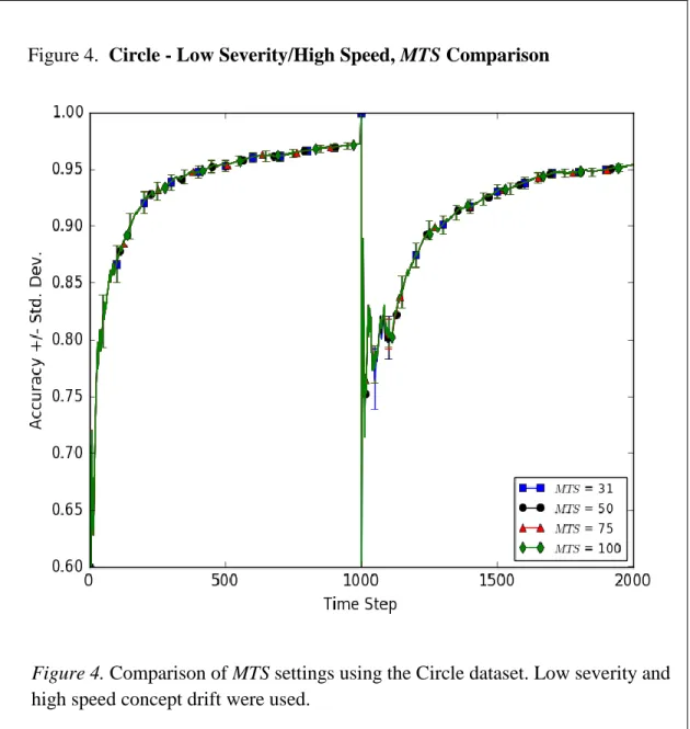
4. Circle - Low Severity/High Speed, MTS Comparison 47 5. Circle - Low Severity/Low Speed, MTS Comparison 48
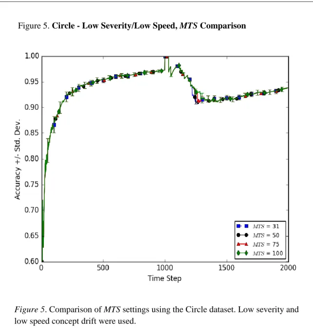
6. Circle - Low Severity/Low Speed, MTS Comparison (Magnified) 49 7. Circle - High Severity/High Speed, MTS Comparison 50
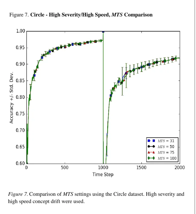
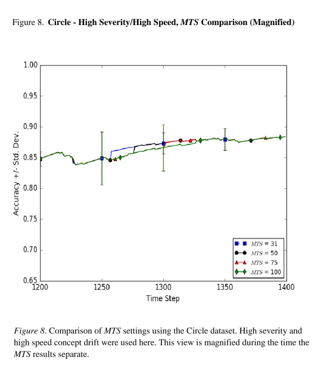
8. Circle - High Severity/High Speed, MTS Comparison (Magnified) 51 9. Circle - High Severity/Low Speed, MTS Comparison 52
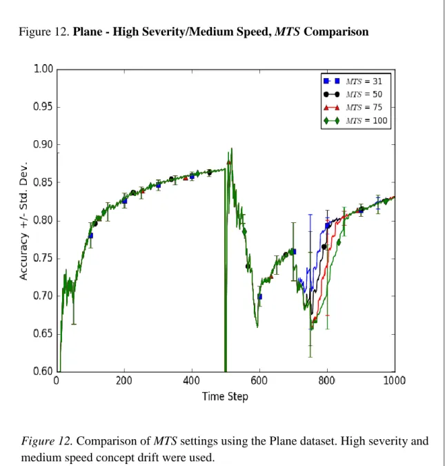
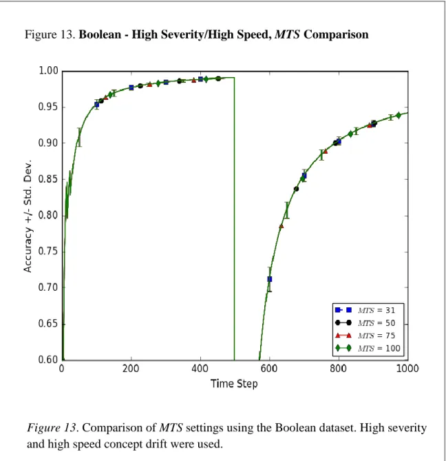
10.SineV - High Severity/Medium Speed, MTS Comparison 53 11.SineH - High Severity/Low Speed, MTS Comparison 54 12.Plane - High Severity/Medium Speed, MTS Comparison 55 13.Boolean - High Severity/High Speed, MTS Comparison 56 14.Frequency of MTS Values for Artificial Data 57
15.Electricity, MTS Comparison 58
16.Forest CoverType, MTS Comparison 59 17.KDD 1999, MTS Comparison 60
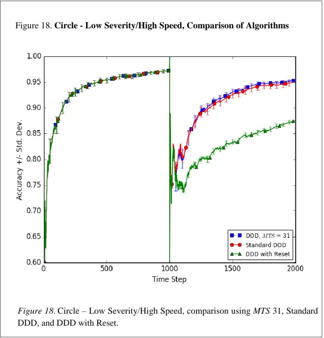
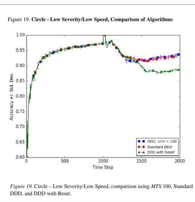
18.Circle - Low Severity/High Speed, Comparison of Algorithms 62 19.Circle - Low Severity/Low Speed, Comparison of Algorithms 63 20.Circle - High Severity/High Speed, Comparison of Algorithms 64 21.Circle - High Severity/Low Speed, Comparison of Algorithms 65 22.SineV - Medium Severity/High Speed, Comparison of Algorithms 66
23.Line - Medium Severity/High Speed, Comparison of Algorithms 67 24.Plane - High Severity/Medium Speed, Comparison of Algorithms 68 25.Boolean - Medium Severity/High Speed, Comparison of Algorithms 69 26.SineH - Low Severity/Low Speed, Comparison of Algorithms 70
27.Circle - Comparison of Average Number of Time Steps in Four Ensembles 72 28.Electricity - Comparison of Algorithms 73
29.Forest CoverType - Comparison of Algorithms 74 30.KDD 1999 - Comparison of Algorithms 75
31.Real World Data - Average Number of Time Steps in Four Ensembles 77 32.Circle - Low Severity/High Speed, Comparison of W values 79
33.Circle - Low Severity/Low Speed, Comparison of W values 80 34.Circle - High Severity/High Speed, Comparison of W values 81 35.Circle - High Severity/Low Speed, Comparison of W values 82 36.SineV - Medium Severity/Low Speed, Comparison of W values 83 37.SineH - Low Severity/High Speed, Comparison of W values 84 38.SineH - Medium Severity/Low Speed, Comparison of W values 85 39.Line - Medium Severity/High Speed, Comparison of W values 86 40.Plane - High Severity/Medium Speed, Comparison of W values 87 41.Electricity - Comparison of W values 88
42.Forest CoverType - Comparison of W values 89 43.KDD 1999 - Comparison of W values 90
List of Algorithms
Algorithms
1. An overview of the DDD algorithm 6 2. An overview of the DWM algorithm 23 3. Modified Online Bagging 25
Chapter 1
Introduction
Background
Supervised machine learning methods are used to determine relationships
between input and output variables based on available observations. The goal is to come up with a function able to predict the output based on the given inputs. When the output variable is categorical, the learned function is said to be a classifier. Traditionally, classifiers are trained in a batch mode using all available observations. In recent years online learning techniques have been developed to deal with applications where observations become available sequentially, one at a time. Restrictions on time and on computing resources prevent machine learning methods to store and process more than a limited number of observations in a batch mode. The applications for online learning have grown in recent years and include such areas as credit card transaction flows, computer security, industrial process control, and intelligent user interfaces. In these systems, data tends to occur in a continuous stream, making storage and repeated processing difficult.
In online learning, the underlying relationships between the input and the output variables may change over time. This is called concept drift. A concept may be
characterized as a joint distribution of the input and output variables. A change in this joint distribution is characterized as a concept drift.
Among the most successful methods to deal with concept drift in online learning is the one proposed by Minku and Yao (2012). Their method uses multiple ensembles, each consisting of online classifiers; the predicted class is the mode class or a weighted average of the constituent classifiers in the ensembles. Using a set of diverse classifiers
with different strengths and weaknesses resulted in the classification accuracy of the ensembles to be significantly greater than any of its constituent classifiers.
The work of Minku and Yao (2012) focused on the use of diversity in ensembles to provide improved accuracy in the presence of concept drift. Since concept drift can have different speeds and severities, it was found that multiple ensembles of varying diversities provided superior accuracy to other drift handling approaches. Their approach improved upon previous methods, but required two ensembles before concept drift was detected (when the concept is stable) and four ensembles after concept drift occurred. Computational overheads are associated with maintaining ensembles. Since an additional two ensembles were required after concept drift, the question of how long these two additional ensembles should remain in memory deserves further investigation. This dissertation will systematically investigate how decisions regarding maintenance of additional ensembles affect the accuracy of ensemble classifiers. The rest of this section discusses the role of diversity in online ensemble classifiers and introduces the algorithm developed by Minku and Yao (2012).
For this study, online learning systems are ones where training examples are processed once on arrival and are not stored. A current hypothesis representing all training instances so far can be maintained by the system. A hypothesis is a function that maps the input variable to an output class. Hypotheses are updated as new training observations arrive. This approach is described by Oza and Russell (2001) and Fern and Given (2003); details are provided in the literature review section.
Work by Fern and Givan (2003) showed how ensembles of small trees provided improvement in classification accuracy over a single tree. Wang, Fan, Yu, and Han (2003) demonstrated the error reduction property and showed that a classifier ensemble can improve upon a single classifier when concept drift is present. Their research found that an ensemble classifier can reduce classification error by making the weight of the
classifier inversely proportional to the expected error of the classifier. Research by Oza and Russell (2001) produced online versions of the ensemble methods bagging and boosting, allowing the benefits of ensemble learning to extend to an online environment.
There are two major approaches for using ensemble methods to detect concept drift. The first approach includes a mechanism to detect drifts explicitly. Here a measure is typically used to determine if a concept drift has occurred. If a concept drift is detected, a new online ensemble of classifiers is created and all classifiers in the ensemble are re-trained. This approach tends to react quickly to concept drift if it is found early. One example of this technique is the work by Baena-García, Del Campo-Ávila, Fidalgo, and Bifet (2006), called the Early Drift Detection Method (EDDM). With this approach it is assumed that the difference in time between consecutive errors will increase when a stable concept is in the process of being learned.A noticeable drop in this difference in time between consecutive errors is considered a concept drift. A new classifier system is generated at this point.
The second approach handles concept drift implicitly. Here weights are assigned to the classifiers of each ensemble and these weights are based on accuracy of the classifiers. Representative of this approach is the work of Kolter and Maloof (2007). Their Dynamic Weighted Majority (DWM) ensemble set up a group of weighted classifiers. Classifiers were added and deleted based on the effectiveness of those classifiers. Classifier weight was reduced if an example was misclassified. In addition, the classifiers which performed poorly were removed from the ensemble if their weights fell below a predefined threshold.
Minku, White, and Yao (2010) discussed the use of diversity to aid online learning where concept drift was found. Their study indicated that a range of diversity levels used with old and new concepts allowed for improved generalization. These diversity levels reflect the degree of agreement between constituent classifiers in the
ensemble. When pairs of classifiers tend to agree, these classifiers are considered less diverse. This study revealed that diversity aided in reduction of error at the beginning of concept drift but did not help improve long-term recovery from concept drift.
The work by Minku and Yao (2012) found that different levels of ensemble diversity used with old and new concepts allowed for improved generalization and gave the maximum prequential accuracy. Prequential accuracy is defined by Dawid and Vovk (1999) as the average accuracy computed from each example presented for training, prior to the example being learned. Prequential accuracy assumes that prediction can be
improved by mapping the prediction to a one-step ahead forecasting system.
It has been shown (Minku & Yao, 2012) that old concept knowledge is useful in new concept learning. They found that high diversity ensembles trained on the old concept could converge to the new concept when the learning of the new concept occurred with low diversity.
The timeline in Figure 1 illustrates their approach to concept drift. As shown, two ensembles are created, one with low diversity and the other with high diversity. After concept drift is detected, two additional ensembles are maintained until the concept is stable. At this point only two ensembles are used.
Figure 1. Concept Drift Detection with DDD
hnl – new low diversity ensemble hol – old low diversity ensemble hnh – new high diversity ensemble hoh – old high diversity ensemble
0 N 2N
Figure 1. Timeline showing how the number of ensembles changes from two to four when concept drift is detected. Data transmission begins at time 0, concept drift occurs at time N, and data transmission is completed at time 2N.
Minku and Yao (2012) developed an algorithm called Diversity for Dealing with Drifts (DDD) as an online ensemble learning approach. The DDD algorithm is
summarized in Algorithm 1. Create hnl and hnh Copy hnl to hol Copy hnh to hoh hnl and hnh Create new hnl and hnh Continue with hnl and hnh only Actual Concept Drift Concept Drift Detected Concept is Stable
Algorithm 1. An overview of the DDD algorithm
1: create new low diversity ensemble hnl and new high diversity ensemble hnh
2: set all ensemble statistics to 0 3: while more data
4: get the next example d 5: if mode==before_drift then 6: make prediction with hnl(d)
7: else
8: make prediction with Weighted Majority of ensembles using d 9: end if
10: test for drift using hnl 11: if drift==true then
12: create old low diversity ensemble hol from either hnl or hoh, depending 13: on accuracy and current mode
14: copy hnh to hoh , making the new high diversity ensemble 15: the old high diversity ensemble
16: create new low diversity ensemble hnl and new high diversity ensemble hnh 17: reset all ensemble statistics to 0
18: mode = after_drift 19: end if
20: if mode==after_drift then
21: if hnl has the highest accuracy then 22: mode = before_drift
23: else
24: if hol has the highest accuracy then
25: copy hol to hnl making the old low diversity ensemble 26: the new low diversity ensemble
27: mode = before_drift 28: end if
29: end if 30: end if
31: do ensemble learning for hnl and hnh 32: if mode==after_drift then
33: do ensemble learning for hol and hoh 34: end if
35: if mode==before_drift then 36: output hnl and prediction 37: else
38: output hnl, hol, hoh, their weights, and their prediction 39: end if
40: end while
Algorithm 1 shows that only two ensembles are created in before-drift-mode (line 1). These ensembles are the new low diversity ensemble and the new high diversity ensemble. Predictions in DDD are made with the new low diversity ensemble in before-drift-mode and with a weighted majority of ensembles when in after-before-drift-mode (lines 5-9). When concept drift is detected, two additional ensembles join the system, one with low diversity and the other with high diversity (line 16). Also, when a drift is detected, the algorithm assigns the old low diversity ensemble used prior to drift detection either to
the new low diversity ensemble or the old high diversity ensemble, choosing the one with the highest accuracy (lines 12-13). In before-drift- mode, ensemble learning occurs only with the two ensembles initially created, one with low diversity and the other with high diversity (line 31). After the concept drift is detected and until the concept is stable, all four ensembles do ensemble learning (lines 31-34). In each time step the output of the learner is displayed. In before-drift-mode, this output comes from the new low diversity ensemble (line 36). In after-drift-mode, the output is weighted by the new low diversity ensemble, the old low diversity ensemble, and the old high diversity ensemble (line 38). While the DDD algorithm has a minimum for the number of time steps to keep four ensembles after a drift is detected, a parameter limiting the maximum number of time steps all four ensembles are in memory is not implemented in the algorithm. The addition of this parameter and its role in the improvement of classifier accuracy was the major focus of this dissertation.
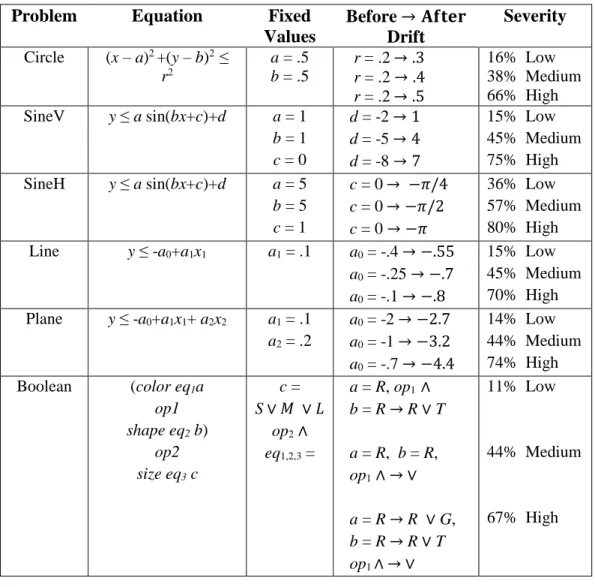
The DDD algorithm was tested with both real world and artificial data. The artificial data contained low, medium, and high severity and low, medium, and high speed. Severity is defined as the percentage of input data that has its target class modified when the drift is complete. Table 1 shows severity for the artificial datasets Circle and SineV used by Minku and Yao (2012). In the dataset Circle, for example, 16% of the input data had its target class modified when the radius r changed from .2 to .3 in the Circle formula, representing low severity. Likewise, 38% of the input data had its target class modified when r changed from .2 to .4 in the Circle formula, indicating medium severity.
Table 1. Examples of Severity
Problem Equation Fixed Values Before → 𝐀𝐟𝐭𝐞𝐫 Drift Severity Circle (x – a)2 +(y – b)2 ≤ r2 a = .5 b = .5 r = .2 → .3 r = .2 → .4 r = .2 → .5 16% Low 38% Medium 66% High SineV y ≤ a sin(bx+c)+d a = 1 b = 1 c = 0 d = -2 → 1 d = -2 → 4 d = -2 → 7 15% Low 45% Medium 75% High
Drifting time is the number of time steps needed for the new concept to take the place of the old one. The inverse of drifting time is the speed of the concept drift. Speed was modeled by the degree of dominance of the new and old concepts defined by Narasimhamurthy and Kuncheva (2007). Drifting time took on the values 1, 0.25N, and 0.5N to allow for the creation of fast, medium, and slow speeds. Minku and Yao (2012) joined {low, medium, high} speed with {low, medium, high} severity to create nine ways to test for varying types of concept drift.
Problem Statement
An unanswered question relates to the tradeoff between improved accuracy and the increased resources necessary to maintain the four ensembles. Is it necessary to maintain the four ensembles the entire time between drift detection and the return to a stable mode? Specifically, how do the number of time steps in the after drift detection mode affect the performance of an online ensemble classifier? Is it possible to maintain the four ensembles in DDD a shorter time to improve resource usage while maintaining prequential accuracy?
Dissertation Goal
In order to study these questions in detail, a parameter which controls the maximum number of time steps the four ensembles are maintained was introduced. A range of values for this parameter was studied. The drift conditions tested reflected those of Minku and Yao (2012) and included both artificial and real world test data. Artificial data was broken down by speed and severity as was described in the introduction. Real world datasets were analyzed in a manner similar to that of Minku and Yao (2012).
Relevance and Significance
As stated earlier, online learning applications have grown in recent years and include such areas as credit card transaction flows, computer security, industrial process control, and intelligent user interfaces. Part of an intelligent user interface could be access to streaming news. The survey by Gama, Žliobaitė, Bifet, Pechenizkiy, and Bouchachia (2014) gives the example that while incoming news items might not change, the
distribution of news items found to be interesting and not interesting for a specific user can change. This is an example of concept drift. This survey also noted that the amount of concept drift research has greatly increased in the last ten years, illustrating the importance of concept drift in online learning.
The research I built on (Minku & Yao, 2012) is mentioned as a “notable technique” in the Gama et al. (2014) survey. Minku and Yao (2012) build on earlier successful concept drift detection techniques giving improved or comparable results, depending on the severity and the speed of the concept drift.
Barriers and Issues
The survey on concept drift by Gama et al. (2014) mentions that while interest in concept drift is growing, the appearance of concept drift in multiple problem domains creates an inconsistency in terminology and techniques. Research has also found that concept drift can vary both by the severity of the drift and by the speed at which the drift occurs. Minku and Yao (2012) used low, medium, and high severity training sets along with low, medium, and high speed training sets to study the impact of low and high diversity ensembles with concept drift.
Also, it is hard to predict if and when concept drift will occur. To aid with this prediction, artificial datasets with build-in concept drift are used for analysis purposes. To help confirm results, real world datasets are also used. An additional issue is the possibility of the detection of concept drift where it does not exist, a false positive. This dissertation attempted to improve on or equal the accuracy of the DDD algorithm of Minku and Yao (2012) with the addition of a maximum on the number of time steps four ensembles used. This maximum on the number of time steps was also studied in situations where false concept drift was present.
Assumptions, Limitations, and Delimitations
The focus of this study is online supervised learning using classification (having discrete outcomes), as opposed to regression (having continuous outcomes). Though the study is restricted to classification, it is believed that results can also be extended to regression. The goal in the study is to make improvements in algorithm accuracy, not speed. Since speed will not be examined, multiple computers will be used in the testing phase.
Summary
In summary, the advantages of maintaining four ensembles after concept drift was detected have been shown by Minku and Yao (2012). These advantages include robust accuracy detection for a variety of drift types and excellent accuracy in the absence of concept drift and when false positive concept drifts appear. Since the benefits of using four ensembles is apparent but more resource intensive than EDDM and DWM, a parameter to control the maximum number of time steps the four ensembles are in
memory will help provide an answer to the question of how long the four ensembles need to be present to provide good accuracy.
Definition of Terms
Table 2. Definition of Terms
Term Definition
Classification Supervised learning with a categorical variable
Controlled Permutation Using randomized copies as in cross-validation
DDD Diversity for Dealing with Drifts algorithm
Diversity levels Degree of agreement between constituent classifiers in the ensemble
Drifting Time Number of time steps needed for the new concept to take the place of the old one
DWM Dynamic Weighted Majority
EDDM Early Drift Detection Method
Holdout A subset of training and testing data is used for testing
Incremental Learning Processes occurring in batches
ITI Incremental Tree Inducer
kappa-statistic Measures the accuracy of an intelligent classifier
Term Definition
Online Bagging Training ensembles by sending K copies of the new example, based on a Poisson distribution Online Learning All training data does not need to be available at
the beginning
Poisson Distribution A discrete probability distribution used in DDD to create diversity in ensembles
Prequential Accuracy Average accuracy of predicted examples, prior to the examples being learned
Q Statistic Measures diversity in ensembles
RAM-hours Computed from the rental cost in a cloud-computing environment
Real Concept Drift A change in the probability of a class occurring
Regression Supervised learning with a continuous output variable
ROC curves Receiver Operating Characteristic curves
Semi-Supervised Learning
Uses a combination of labeled and unlabeled examples for learning
Severity Percentage of input data that has its target class modified when the drift is complete
Speed The inverse of drifting time
Term Definition
Unsupervised Learning Does not have labeled data in its training data
Virtual Concept Drift The input data changes but the boundary between class labels does not change
W Multiplier on the weight of the old low diversity ensemble, used for false positive concept drift
Chapter 2
Review of the Literature
Overview
This section begins with a justification of the criteria for the research included and excluded in the review. Then background for machine learning, supervised learning, and concept drift will be presented. After that the highlights of concept drift research will be given, followed by key work where ensembles were used to handle concept drift. Then research that has been done by adding diversity in ensembles to handle concept drift will be shown. Following will be a discussion of work done on how to minimize the impact of false positive concept drift on classifier accuracy. Finally, a review of common
performance evaluation techniques used in concept drift research will be presented.
Justification of Review Criteria
As shown in the survey by Gama et al. (2014), research in the area of concept drift research is strong and growing, but it is also fragmented into different problem domains. Also, there is disagreement among researchers in this field regarding terminology. Since concept drift research covers a broad area, this review will not be exhaustive. Beyond the highlights of concept drift research, the primary criteria for this review will be how close specific research papers are to my dissertation topic. For example, research on the memory of a predictive model is related to concept drift but falls outside of my research focus, as does work on reoccurring concept management. Included would be work done on concept drift detection and learning.
Types of Machine Learning
The goal in machine learning is for computer programs to automatically find patterns and learn to recognize concepts from data (Han, Kamer, & Pei, 2012). The three major types of machine learning are supervised learning, unsupervised learning, and semi-supervised learning. Supervised learning has labeled data in its training data so that as training occurs, the correct response is available. If the target to predict is a categorical variable, this process is called classification. If the variable is continuous the process is called regression. With unsupervised learning, the class labels are not known. An
unsupervised learning model identifies clusters of data and therefore creates its own class labels. Semi-supervised learning uses a combination of labeled and unlabeled examples for learning. For this dissertation, supervised learning using classification will be used. Duda, Hart, and Stork (2001) describe classification using Bayesian Decision Theory through the prior probabilities for classes 𝑝(𝑦)and the class conditional probability
𝑝(𝑋|𝑦). These values are used to compute the posterior probability of the classes, given
by:
𝑝(𝑋|𝑦) = 𝑝(𝑦) 𝑝(𝑋|𝑦)
𝑝(𝑋)
Here 𝑝(𝑋) is defined as:
∑ 𝑝(𝑦) 𝑝(𝑋|𝑦) 𝑐
𝑦=1
where c is the number of output classes, X is the input value, and y is the class label.
Strategies for Supervised Learning
Broad categories of supervised learning are offline learning and online learning. In offline learning, the entire training set needs to be available before predictions can be
made. With online learning, all of the training data does not need be available at the beginning. With online learning the learning model is updated as more training data enters the system. Variations of online learning include incremental learning and stream learning. Incremental learning is defined by processes occurring in batches, providing a way to not have the entire training set available like offline learning and without
including the restriction of sequential processing found in online learning. With incremental learning, the system may be updated by referring to previous examples. Finally, stream learning algorithms process incoming data sequentially like online learning but the data is also continuous and high speed. Because of these requirements, stream learning algorithms must perform with low memory and low processing time. The focus of this dissertation will be online learning where data enters the system in the form of a data stream.
Definition of Concept Drift
In situations where data streams occur, the underlying data distribution can change. For example, Kolter and Maloof (2007) use the example of a professor’s email classification system. The types of email identified as “important” and “not important” will change as semesters change and as conference deadlines come and go. When these class labels change over time, this is considered concept drift.
Mathematically, concept drift can be defined as:
where 𝑝𝑡0is the joint distribution at time 𝑡0 of the input set 𝑋 and the target 𝑦. Kelly, Hand, and Adams (1999) mention that concept drift can change the probabilities of classes 𝑝(𝑦|𝑋), leading to misclassification of the target variable 𝑦. Specifically, this change is called real concept drift (Gama et al., 2014). A second kind of drift called
virtual concept drift is defined as a change in 𝑝(𝑋) without a change in 𝑝(𝑦|𝑋)
(Tsymbal, A., 2004; Widmer & Kubat, 1993). Figure 2, from Gama et al. (2014), shows how class boundaries and labels change during real concept drift and virtual concept drift.
Figure 2. Types of Drifts
Original Data Real Concept Drift Virtual Concept Drift
𝑝(𝑦|𝑋) changes 𝑝(𝑋) changes, but not 𝑝(𝑦|𝑋) Figure 2. These graphs show types of drifts. The circles represent instances,
different colors representing different classes, and dotted lines representing class boundaries (adapted from Gama et al., 2014).
In Figure 2, with real concept drift the boundary between the class labels changes but the input data does not change. When virtual concept drift occurs, the input data changes but the boundary between class labels does not change. Most of the concept drift research refers to real concept drift. The work in this study will focus on real concept drift and future references to concept drift will imply real concept drift.
Highlights in Concept Drift Research
The first work on concept drift was by Schlimmer and Granger (1986). Their approach used a set of weighted symbolic characteristics to describe concepts. Learning systems were then used to adjust these weights and create new characterizations to describe the concepts. This technique, known as STAGGER, served as the basis for later studies. Klenner and Hahn (1994) used frame representation to handle gradual concept drift. Widmer and Kubat (1996) created a system, called FLORA, that dynamically adjusted a window of time to refine positive, negative, and potential rules in order to track concept drift. Widmer (1997) used naïve Bayes and meta-learning to handle reoccurring concepts. Klinkenberg and Joachims (2000) studied the use of a support vector machine to size windows for concept drift. A concept-adapting Very Fast Decision Tree (CVFDT) learner (Hulten, Spencer, & Domingos, 2001) added concept drift to the work on VFDT (Domingos & Hulten, 2000). Chandola, Banerjee and Kumar (2009) explored the challenge of confusing concept drift with an outlier or noise.
Ensemble Methods with Concept Drift
Ensemble methods have proven to perform well with concept drift and
researchers have created online versions of popular ensemble methods, such as online AdaBoost (Fan, Stolfo, & Zhang, 1999). As mentioned earlier, Fern and Givan (2003) provided evidence that ensembles of small trees gave greater classification accuracy than a single tree. Wang et al. (2003) showed that a classifier ensemble can improve on a single classifier when concept drift is present. Gao, Fan, and Han (2007) suggested that unweighted ensembles may be beneficial in the presence of concept drift. Blum (1997) used an incremental approach to concept drift. Here experts were created from pairs of attributes and predictions were made by using majority vote (Littlestone & Warmuth,
1994) from the results of all possible pairs. After the system received the correct class label, experts that predicted incorrectly had their weights cut in half. Other research conducted using ensemble methods to discover concept drift include work by Street and Kim (2001). Their Streaming Ensemble Algorithm (SEA) approach used a fixed-size collection of classifiers built from training examples. When new examples appeared a new classifier was created and the new classifier was added to the ensemble if room was available. If room was not available, a poorer performing classifier was removed to make room for the new classifier. Predictions were made by majority vote. Scholz and
Klinkenberg (2006) created two ensembles and then chose the best for later processing.
Concept Drift Detection
There are two major classifications of strategies for using ensemble methods to detect concept drift according to the research of Minku and Yao (2012). One ensemble approach to check for concept drift is to include a mechanism to detect drifts explicitly. Here a measure is typically used to determine if a concept drift has occurred. If a concept drift is detected, a new online classifier is created and all classifiers in the ensemble are re-trained. This approach tends to react quickly to concept drift if it is found early. On the negative side, the explicit approach can sometimes detect a drift where a drift has not occurred. One example of this explicit technique is the work by Baena-García, Del Campo-Ávila, Fidalgo, and Bifet (2006), called the Early Drift Detection Method
(EDDM). With this approach it is assumed that when a stable concept is in the process of being learned, the difference in time between consecutive errors will be larger. A
noticeable drop in this difference is considered a concept drift. A new classifier system is generated at this point.
The second approach handles concept drift implicitly. Here it is common to attach weights to the classifier of each ensemble. These weights are based on accuracy and provide for addition and deletion of new classifiers. Representative of this approach is the work of Kolter and Maloof (2007). Their Dynamic Weighted Majority (DWM) ensemble set up a group of weighted classifiers. Classifiers were added and deleted based on the effectiveness of those classifiers. Classifier weight was reduced if a mistake was made. In addition, the experts which performed poorly were deleted if their weights fell below a predefined threshold. The downside of this approach is that time is required for the classifier weights to represent the new concept.
EDDM
Concept drift can occur abruptly or gradually. The method used by Gama, Medas, Castillo, and Rodrigues (2004) detected concept drift by counting the number of errors found in examples. This method worked well for abrupt concept drift but did not achieve good performance if the drift was gradual. Gradual concept changes are more difficult to detect, partly because of the need for increased resources to store additional examples. As stated earlier, the EDDM algorithm (Baena-García et al., 2006) identified concept drift by keeping track of the number of time steps between classification errors. EDDM used a warning threshold and a concept drift threshold to determine when a new concept was present. If the warning threshold was reached, examples were saved in preparation for new concept learning. If the concept drift threshold was met, the old learning model was reset and a new learning model was created using the examples saved after the warning threshold was reached. EDDM performed well on both abrupt and gradual drifts when compared to similar drift detection methods. Following are the calculations used with warning level (α) and drift level (β):
(𝑝𝑖′ + 2𝑠
𝑖′)/(𝑝𝑚𝑎𝑥′ + 2𝑠𝑚𝑎𝑥′ ) < 𝛼 (for the warning level) (𝑝𝑖′ + 2𝑠
𝑖′)/(𝑝𝑚𝑎𝑥′ + 2𝑠𝑚𝑎𝑥′ ) < 𝛽 (for the drift level)
Here 𝑝𝑖′ is the average difference in time steps between errors in classification and
𝑠𝑖′ is the standard deviation of this average. Also, 𝑝
𝑚𝑎𝑥′ and 𝑠𝑚𝑎𝑥′ hold the highest values
of 𝑝𝑖′ and 𝑠𝑖′, respectively. Calculations are done after 30 errors have occurred. The number 30 was chosen so a distribution of error differences can be compared to other distributions. The denominator 𝑝𝑚𝑎𝑥′ + 2𝑠𝑚𝑎𝑥′ represents 95% of the distribution. Figure
3 shows how the thresholds 𝛼 and 𝛽 are used in EDDM.
Figure 3. Concept Drift Detection with EDDM
0 𝛽 𝛼 1
Figure 3. This is a description of the relationship between 𝛼 and 𝛽 in the EDDM algorithm.
As can be seen in Figure 3, the system runs normally from a value of 𝛼 and above. Examples are stored when the threshold is between 𝛼 and 𝛽. Results below 𝛽
Concept drift has been detected. Create new model, learn from stored examples
Store examples, concept drift may be coming
Remove stored examples if they exist and return to normal
signal that a concept drift has been detected. At this point the current model is reset and a new model learns using the stored examples.
DWM
As mentioned earlier, concept drift can also use implicit concept drift detection. Algorithm 2 shows the DWM algorithm of Kolter and Maloof (2007).
Algorithm 2. An overview of the DWM algorithm
1: create New Expert with Weight = 1
2: for all Examples
3: set Sum of Weighted Predictions for each class to 0
4: for all Experts
5: resultFromClassify = classify(expert, example)
6: if resultFromClassify not correct and not in Waiting Period then 7: decrease weight by factor of β (0 ≤ β < 1)
8: end if
9: compute Sum of Weighted Predictions for each class 10: end for
11: get class with the highest weight 12: if not in Waiting Period then
13: normalize weights (maximum weight is one) 14: remove experts with weight less than 𝛩
15: if class with highest weight ≠ correct class then 16: create New Expert with Weight = 1
17: end if 18: end if
19: for all Experts 20: train expert 21: end for
22: output class with Highest Weight 23: end for
Algorithm 2 begins with the creation of a single ensemble with a weight of one (line 1). The current example is then given to the expert for classification (line 5). If the classification is not correct, the expert’s weight is decreased by a factor of β (lines 6 and 7). A weighted sum is then computed for each class (line 9). The class with the highest weight (line 11) is identified as the global prediction. Weights of ensembles are
normalized so they can be compared (line 13) and poorly performing experts are removed (line 14). If the global prediction (class with the highest weight) is incorrect, a new expert is created (lines 15 and 16). DWM includes a parameter for a waiting period. During the waiting period, the weights of experts are not changed and experts are not added and deleted (lines 6 and 12).
Diversity with Ensembles
The use of diversity in base classifiers of ensembles has been studied. The ensemble techniques of bagging and boosting utilized a diverse set of classifiers. Dietterich (2000) tested the randomization, bagging, and boosting ensemble techniques and found that when classification noise was present, bagging out-performed boosting and randomization in most cases. In the presence of noise, bagging appeared to be able to use the classification noise to its advantage. The study by Breiman (2001) found that random forests with lower error tended to have lower base classifier correlation and higher classification accuracy. Guerra-Salcedo and Whitley (1999) used a generic algorithm (GA) to create the components of an ensemble. Their results revealed that diversity created by the GA improved on that of random ensembles. The research of Kuncheva and Whitaker (2004) identified that diversity in ensembles was important but that it was difficult to measure diversity. The addition of ensembles with high and low diversity levels was explored by Minku and Yao (2012) and their results improved on work from similar studies.
Minku and Yao (2012) found that a range of diversity levels in ensembles gave the maximum prequential accuracy.
Prequential accuracy was described by Dawid and Vovk (1999) and is the average accuracy of predicted examples, prior to the examples being learned and is computed by: 𝑎𝑐𝑐(𝑡) = { 𝑎𝑐𝑐𝑒𝑥(𝑡), 𝑖𝑓 𝑡 = 𝑓, 𝑎𝑐𝑐(𝑡 − 1) + 𝑎𝑐𝑐𝑒𝑥(𝑡) − 𝑎𝑐𝑐(𝑡 − 1) 𝑡 − 𝑓 + 1 , 𝑜𝑡ℎ𝑒𝑟𝑤𝑖𝑠𝑒,
In this equation 𝑎𝑐𝑐𝑒𝑥 is 0 when the prediction of the current training example 𝑒𝑥
is incorrect and 1 if the training example is correct, 𝑓 is the first time step used when calculating the data, and t is the time step. Minku & Yao (2012) studied the ensembles used both before and after the start of concept drift. As part of this analysis, prequential accuracy was reset when the drift began (𝑓 ∈ {1, 𝑁 + 1}). Here N represents the number of time steps before the concept drift began.
Diversity levels were controlled in DDD using a modified version of the
algorithm from Minku, White, and Yao (2010). Their work was influenced by the online bagging technique of Oza and Russell (2001). This technique is shown in Algorithm 3.
Algorithm 3. Modified Online Bagging
1: for each base_learner hm in ensemble h
2: get K copies of the training example d from a Poisson(1) distribution
3: while K > 0
4: update the base learner hm using OnlineBaseLearningAlgorithm(hm,d)
5: K = K - 1 6: end while 7: end for
Algorithm 3 uses the idea that as the number of training examples gets large, each base learner holds K copies of the original training example (lines 3-6). It turns out that the distribution of K looks like a Poisson(1) distribution, so as new examples are obtained, the
number of times each base learner sees the example is taken from a Poisson(1)
distribution (line 2). The calculation of K can be changed to Poisson(λ) to create diversity in ensembles. A higher λ gives lower diversity and a lower λ gives higher diversity.
To measure diversity, Minku and Yao (2012) followed the recommendation of Kuncheva and Whitaker (2003) and used Yule’s Q statistic (1900) which follows:
𝑄𝑖,𝑘 = 𝑁11𝑁00− 𝑁01𝑁10
𝑁11𝑁00+ 𝑁01𝑁10
Given two classifiers Di and Dk, Na,b was the number of training examples where the classification of Di is a and the classification of Dk was b. Here 1 was a correct classification and 0 was an incorrect classification. Q values were in the range [-1,1] and tended to be positive the more classifiers agreed on a classification. In the study by Minku and Yao (2012), the Q statistic was averaged over every pair of classifiers to provide a metric for diversity. A high average Q statistic represented low diversity and a low average Q statistic represented high diversity.
DDD Algorithm
In the DDD algorithm of Minku and Yao (2012), discussed in chapter 1, two ensembles were used before concept drift was detected, one with low diversity and the other with high diversity. If concept drift was detected, two additional ensembles were created. One of these had low diversity and the other had high diversity. These four ensembles remained in memory until either of the following conditions occurred: The new low diversity ensemble had better accuracy than either of the two old ensembles or the old high diversity ensemble had better accuracy than the new low and old low diversity ensembles. It is not known if placing a maximum limit on the number of time steps these four ensembles were in memory would provide comparable accuracy. If this
maximum limit on time steps does provide comparable accuracy, it would be an improvement on the current method in two ways. First, memory usage should decrease because the additional ensembles would need to be in memory a shorter time. Second, the time the DDD algorithm takes to run should decrease because the two additional
ensembles would not have to be maintained as long. Since this extra maintenance would not be required, less processing would be needed and run time should go down.
False Positives in Concept Drift
It is important for a learning system to be accurate in the presence of concept drift, and it is also important to keep concept drift from being detected when it is not present. Minku and Yao (2012) addressed this issue by using an additional parameter, named W, as a multiplier on the weight of the old low diversity ensemble. Increased values of W allowed DDD to detect concept drift false alarms more easily, but accuracy was sacrificed when real concept drift occurred. A lower value for W made DDD less able to detect false alarms, but accuracy improved with this lower setting when real concept drift arose.
Comparison of EDDM, DWM, and DDD
Minku and Yao (2012) compared the DDD, EDDM, and DWM algorithms. Different diversity levels were used with DDD to test the impact of diversity levels on accuracy. In the first concept, DDD and EDDM were similar if false positive concept drift did not exist. When there was false positive concept drift, DDD was more accurate than EDDM because EDDM resets its accuracies when a false positive concept drift occurs. In this case the knowledge of the current concept is lost. DDD, on the other hand,
increases the old ensemble weights so that false positive concept drift is less likely in the future.
After concept drift has been detected, DDD performed better than EDDM on most kinds of drifts, because of its ability to learn from the old ensembles. DDD also gave higher accuracy than DWM, whether concept drift was present or not.
Performance Evaluation
When evaluating machine-learning techniques, performance evaluation metrics are needed as well as ways to train and test the machine-learning techniques (Gama et al., 2014). When memory usage is part of the study, RAM-hours have been used as a
performance metric (Bifet, Holmes, Pfahringer, & Frank, 2010). RAM-hours are computed from the rental cost in a cloud-computing environment. The use of one gigabyte of RAM for one hour is one RAM-hour. To compare the accuracy of an intelligent classifier to a random classifier, the kappa-statistic is defined as:
𝑎 − 𝑎𝑟
1 − 𝑎𝑟
where the accuracy of the intelligent classifier is a and the accuracy of a random
classifier is ar. A kappa-statistic closer to 1 indicates the intelligent classifier is closer to a
perfect classifier. A kappa-statistic of 0 means the intelligent classifier is no better than a random classifier. The kappa-statistic has been found to be a good alternative to Receiver Operating Characteristic (ROC) curves when streaming data is being evaluated and classifiers are being compared. Bifet, Holmes, and Pfahringer (2010) used the kappa-statistic to compare leverage bagging and online bagging. Minku and Yao (2012) used t-tests to compare the accuracy of various concept drift techniques. These t-t-tests were done right before concept drift, right after concept drift, a medium time after concept drift, and a long time after concept drift. A common way to measure performance in concept drift
algorithms is by graphing prequential accuracy (defined in Chapter 1) over time steps. Concept drift algorithms that use this approach include: DDD (Minku & Yao, 2012), EDDM (Baena-García et al., 2006), and DWM (Kolter and Maloof, 2007). It is also common to add one ± standard deviation to the average prequential accuracy. Minku and Yao (2012) also graphed the change in weights on the new low, old low, and old high diversity ensembles over time steps.
While supervised learning systems typically use cross-validation to estimate performance with static data, this approach does not translate well with data that contains concept drift. According to Gama et al. (2014), cross-validation could mix the data in such a way that the temporal order of the data would be lost. Three techniques commonly used to determine the data for training and testing are: holdout, prequential, and
controlled permutations. With holdout evaluation, a subset of training and testing data is used for testing. The holdout set maintains the same concepts as does the training and testing sets, only on a smaller amount of data. Prequential evaluation (defined in Chapter 1) allows individual examples to be tested before they are used in the training phase. A holdout set is not required for this technique. Controlled permutations (Žliobaitė, I., 2011) use randomized copies as in cross-validation. The difference is that controlled permutations attempt to keep data in its original position.
Summary
This chapter contains a review of the literature in concept drift research. From this review there is a high likelihood that increases in data stream data will continue to
provide situations where concepts will change over time. It is also clear that there is a strong need for improved algorithms to handle concept drift effectively. In addition, it was shown that an ensemble of classifiers provides better classification accuracy than a
single classifier. Research using diversity in ensembles (Minku & Yao, 2012) was shown to be a promising approach to improved classification. Also, adding additional ensembles appears to provide greater accuracy. There is a tradeoff, however, because the additional ensembles require more time and space resources. A study of the impact on accuracy of placing a maximum on the number of time steps that four ensembles can be in memory appears to be a valid path for continued research.
Chapter 3
Methodology
Overview of Methodology
As described in the problem statement, this dissertation investigated how prequential accuracy in the DDD algorithm is affected by the placement of a maximum on the number of time steps four ensembles are stored in memory. For discussion
purposes this maximum was called the maximum time step parameter and was defined as MTS. A secondary portion of my work examined the impact of changes in the W
parameter with the maximum limit time step parameter included. The W parameter was used in the DDD algorithm as a weight on the old low diversity ensemble to detect false concept drift. This section begins with a broad overview of my dissertation approach. A breakdown of these steps follows. After this, preliminary work done is mentioned and knowledge gained from this work is described. Finally, the details of how results were analyzed is given and a listing of resources used is shown. Here is the broad overview of the method I used in my dissertation:
1. Created an additional parameter to the DDD algorithm that put a maximum limit on the number of time steps four ensembles were in memory when concept drift was detected (the MTS parameter). This parameter took on a range of values to test its impact on prequential accuracy.
2. Tested the DDD algorithm with a range of values in the MTS parameter on the artificial datasets used by Minku and Yao (2012). Low, medium, and high speed concept drift data were used along with low, medium, and high severity concept drift data.
3. Tested a range of values in the MTS parameter using some of the real world datasets found in Minku and Yao (2012), Gama, Rocha, and Medas (2003), and Oza and Russell (2001).
4. Compared the DDD algorithm using the most promising MTS parameter to the DDD algorithm without the MTS parameter and to a version of the DDD algorithm that had its learning reset after concept drift was encountered.
5. Modified the values for the W parameter in the DDD algorithm. The W
parameter was used in the DDD algorithm as a weight on the old low diversity ensemble to help keep the algorithm from reacting to what appears to be a concept drift but is not. The impact of changes in W related to settings in the MTS parameter were explored and were compared to changes in the W parameter using the DDD algorithm without the MTS.
Maximum Time Step Parameter
An additional parameter to the DDD algorithm was created. This parameter placed a maximum on the number of time steps that four ensembles were kept in memory when concept drift was detected. The added code created a condition to return the state of the DDD algorithm to before-drift-mode when the maximum time step was reached. At this point the number of ensembles reduced from four to two.
Testing with Artificial Datasets
Analysis of concept drift with real world datasets is difficult. With real world datasets, the location of and presence of concept drift is not always known. That is why it is common in concept drift research to use artificial data that can be controlled. The artificial datasets used were the same as those used in Minku and Yao (2012). These datasets were circle, sine moving vertically, sine moving horizontally, line, plane, and Boolean. The Boolean dataset was derived from the original STAGGER problem (Schlimmer & Granger, 1986). The attributes color, shape, and size were used with the Boolean dataset to determine if the object was in class 1 or class 0.
Various speed and severity values were used with this artificial data. As
mentioned earlier, speed is the inverse of drifting time, which is the number of time steps needed for the new concept to take the place of the old concept. The degree of dominance of the new and old concepts was defined by Narasimhamurty and Kuncheva (2007).
Here vn(t) is the probability the new concept will be presented to the system and
v0(t) is the probability the old concept will be presented to the system and are defined as:
𝑣𝑛 (𝑡) = 𝑑𝑟𝑖𝑓𝑡𝑖𝑛𝑔_𝑡𝑖𝑚𝑒𝑡 − 𝑁 , 𝑁 < 𝑡 ≤ 𝑁 + 𝑑𝑟𝑖𝑓𝑡𝑖𝑛𝑔_𝑡𝑖𝑚𝑒
and
𝑣0 (𝑡) = 1 − 𝑣𝑛 (𝑡), 𝑁 < 𝑡 ≤ 𝑁 + 𝑑𝑟𝑖𝑓𝑡𝑖𝑛𝑔_𝑡𝑖𝑚𝑒 In these equations, t is the current time step, N is the number of steps before the concept drift, and drifting_time represents the time steps required for the new concept to completely replace the old concept. Each of these artificial datasets contained one
concept drift and contained 2N examples. The old concept 𝑣0 (𝑡) was used for the first N
examples (1 ≤ t ≤ N). The next drifting_time examples used the probabilities of 𝑣0 (𝑡) and
𝑣𝑛 (𝑡) to determine whether to use the old or new concept (N < t ≤ N+drifting_time). After this time, the remaining examples ( N+drifting_time < t ≤ 2N) were generated by the new concept 𝑣𝑛 (𝑡). Speeds for the artificial datasets used drifting_time values of 1, 0.25N, and 0.50N time steps as was done in Minku and Yao (2012). This allowed for the creation of fast, medium, and slow speeds.
As stated earlier, severity is defined as the percentage of input data that has its target class modified when the drift is complete. Table 3 shows the severity changes for all the artificial datasets to be used for this study.
Table 3. Severity for Artificial Datasets Problem Equation Fixed
Values Before → 𝐀𝐟𝐭𝐞𝐫 Drift Severity Circle (x – a)2 +(y – b)2 ≤ r2 a = .5 b = .5 r = .2 → .3 r = .2 → .4 r = .2 → .5 16% Low 38% Medium 66% High SineV y ≤ a sin(bx+c)+d a = 1 b = 1 c = 0 d = -2 → 1 d = -5 → 4 d = -8 → 7 15% Low 45% Medium 75% High SineH y ≤ a sin(bx+c)+d a = 5 b = 5 c = 1 c = 0 → −𝜋/4 c = 0 → −𝜋/2 c = 0 → −𝜋 36% Low 57% Medium 80% High Line y ≤ -a0+a1x1 a1 = .1 a0 = -.4 → −.55 a0 = -.25 → −.7 a0 = -.1 → −.8 15% Low 45% Medium 70% High Plane y ≤ -a0+a1x1+ a2x2 a1 = .1 a2 = .2 a0 = -2 → −2.7 a0 = -1 → −3.2 a0 = -.7 → −4.4 14% Low 44% Medium 74% High Boolean (color eq1a op1 shape eq2 b) op2 size eq3 c c = S ∨ 𝑀 ∨ 𝐿 op2∧ eq1,2,3 = a = R, op1 ∧ b = R→R∨T a = R, b = R, op1∧→∨ a = R→R ∨G, b = R→R∨T op1 ∧ →∨ 11% Low 44% Medium 67% High
Table 3 uses a, b, c, d, r, ai,, eq, and op to define values for equations that
represent different concepts. In the SineV equation, for example, 15% of the input data had its target class modified when the variable d changed from -2 to 1 in the SineV formula. This represents low severity. Also, 45% of the input data had its target class modified when d changed from -5 to 4 in the SineV formula, indicating medium severity. The severity used with these datasets was low, medium and high. Having three settings for speed and three settings for severity allowed for the creation of nine comparisons for each of the artificial datasets. The artificial datasets were tested with Incremental Tree Inducer (ITI) lossless decision trees as base learners (Utgoff, Berkman, & Clouse, 1997). The ensemble size was 25 ITI lossless decision trees and each dataset ran 30 times to
produce the average prequential accuracy. The test values for the MTS parameter were 31, 50, 75, and 100. The selection of 31 was used because 31 is the minimum possible for the DDD, since the DDD algorithm requires the four ensembles to be in memory at least 30 time steps. The other three MTS values (50, 75, 100), where chosen because they are the next three multiples of 25 after the minimum value of 31. The λl low diversity
parameter was set to 1.0 as was done in Minku and Yao (2012). For the λh high diversity
ensembles, this value was 0.05 for circle, sineH, and plane. SineV was set to 0.005 and Boolean was 0.1 for λh high diversity ensembles. These values for the high diversity
ensemble setting λh were the same as those used by Minku and Yao (2012) that showed
good results. Each artificial dataset contained 2N examples; one example represented one time step. Circle, sineV, sineH, and line had an N value of 1000. The N value for both plane and Boolean was 500. Table 4 shows additional settings for the artificial datasets.
Table 4. Settings for Artificial Datasets Dataset Training
File Size
Testing File Size
Range of X Range of Y High Diversity λh Circle 2000 500 [0,1] [0,1] 0.05 SineV 2000 500 [0,10] [-10,10] 0.005 SineH 2000 500 [0,4π] [0,10] 0.05 Line 2000 500 [0,1] [0,1] 0.005 Plane 1000 200 [0,1] [0,5] 0.05 Boolean 1000 200 (R,G,B) Color (T,R,C) Shape (S,M,L) Size [0,1] 0.1
Testing with Real World Data
To be beneficial, new algorithms for concept drift detection need to work with real world data. Some of the same real world datasets used by Minku and Yao (2012) were used in this research. The first of these real world datasets, described by Harries (1999), is an electricity dataset from the Australian New South Wales Electricity Market. The dataset contained 45,312 examples made up of the input attributes: time stamp, day of week, and two electricity demand values. The target class is the change in the price of electricity. Price is affected by supply and demand. During the time period of this dataset (May 1996 to December 1998), an expansion of the electricity area caused a decrease in electricity price. This decrease in price represents concept drift. The second real world dataset was the KDD Cup 1999 network intrusion data (The UCI KDD Archive, 1999). This dataset contains 494,090 examples. The 41 input attributes of this dataset includes
connection length, protocol type, and destination network service. The target class is connection status (attack or normal). This dataset simulates a military environment where attacks were so common that attack occurred more frequently than did normal. The third real world dataset was the Forest Covertype dataset (Asuncion & Newman, 2007). This dataset has been used by other concept drift researchers (Gama, Rocha, & Medas, 2003; Oza & Russell, 2001). Forest Covertype is made of 30 x 30 meter cells from the US Forest Service. The dataset contains 581,012 examples with 54 attributes. The class is the type of forest suggested by the attributes. ITI decision trees were used as base learners with the real world datasets. The ensemble size for the ITI decision trees was 25. As with the artificial data, each real world dataset ran 30 times to produce the average prequential accuracy and the values used to test the MTS parameter were 31, 50, 75, and 100. See the previous section for the details that explain the choice of MTS values. Since accuracy and not speed was the focus of this dissertation, a subset of the full real world datasets was used. With all three real world datasets, the training file size was 2000 and the testing file size was 500. These sizes were chosen because they matched the size of four of the six artificial datasets. All three real world datasets used training files created from the first 80% of the original data. The testing files were created from the remaining 20% of the original data. As with the artificial datasets, the low diversity ensemble setting λl was 1.0
for all real world datasets. The real world data high diversity ensembles had the λh setting
of 0.005, the same as used by Minku and Yao (2012) for Electricity and the KDD Cup 1999 datasets. The settings for the real world datasets are found in Table 5.