Munich Personal RePEc Archive
Leveraging Loyalty Programs Using
Competitor Based Targeting
Hollenbeck, Brett and Taylor, Wayne
UCLA Anderson, SMU Cox
March 2020
Online at
https://mpra.ub.uni-muenchen.de/99235/
Leveraging Loyalty Programs Using Competitor Based
Targeting
Wayne Taylor
Cox School of Business
Southern Methodist University
∗Brett Hollenbeck
Anderson School of Management
UCLA
†March 13, 2020
Abstract
Loyalty programs are widely used by firms but their effectiveness is not well understood. These programs provide discounts and perks to loyal customers and are costly to administer, and with uncertain effects on spending or stealing business from rivals. We use a large and detailed dataset on customer shopping behavior at one of the largest U.S. retailers before and after joining a loyalty program to evaluate how behavior changes. We combine this with detailed spatial data on customer and store locations, including the locations of competing firms. We find significant changes in behavior associated with joining the LP with a large amount of heterogeneity across customers. We find that location relative to competitors is the factor most strongly associated with increases in spending following joining the LP, suggesting that the LP’s quantity discounts work primarily through business stealing and not through other demand expansion. We next estimate a set of predictive models to test what variables best predict LP effectiveness using high-dimensional data on spatial relationships between customers, the focal firm’s stores, and competing stores as well as customers’ historical spending patterns. These models are used to test whether past sales data reflecting customer’s vertical value to the firm or spatial data reflecting customer’s horizontal vulnerability are more predictive of LP effects. We show how LASSO regularization estimated on complex spatial relationships are more predictive of LP effects than are models using past sales data or other spatial models including gravity models. Finally, we show how firms can use this type of model to leverage customer and competitor location data to substantially increase the performance of their LP through spatially driven targeting rules.
Keywords: Loyalty programs, predictive analytics, spatial models, retail competition, targeted price discrimination, LASSO estimation
1
Introduction
Loyalty programs are now prevalent in many industries. The loyalty programs as marketers know them today originated in the airlines in the 1980s and have since permeated industries such as hotels, casinos, retailers, grocery stores, and restaurants, among others. The pervasiveness of loyalty programs is partly due to their flexibility in how they can be structured (e.g., earning rates and rewards) and managed for strategic decisions (e.g., targeting to increase customer engagement). In spite of the popularity of loyalty programs with firms, their effectiveness at increasing profits has long been subject to debate. This debate has centered on the costs of giving discounts and perks to the most loyal customers, as well as the costs of administering the program itself, and whether these costs are justified by increases in spending by those customers. Loyalty programs have the potential to increase profits by increasing switching costs for existing customers, stealing business from rivals, or through second degree price discrimination. They may also indirectly increase profits by increasing customers psychological perceptions of the firm, by generating customer data that can be used for targeted promotions or CRM, or by exploiting agency issues such as flights booked by business travelers and paid for by their employers (Dreze and Nunes (2008), Roehm et al. (2002), Verhoef (2003), and Shugan (2005)).1
Empirical studies of whether loyalty programs actually do increase profits have found mixed results. Verhoef (2003) finds that the effects are positive but very small, DeWulf et al. (2001) finds no support for positive effects of direct mail, Shugan (2005) finds that firms gain short term revenue at the expense of longer term reward payments, and Hartmann and Viard (2008) found no evidence that loyalty programs create switching costs.
In this paper, we use a large and detailed dataset on customer shopping behavior at one of the largest U.S. retailers before and after joining a loyalty program. This loyalty program takes a common form, tiered discounts after a certain level of spending, essentially operating as 2nd degree price discrimination or one particular form of behavior-based pricing (BBP). We therefore analyze the program through the lens of theoretical work in marketing on price discrimination and BBP, most notably Shin and Sudhir (2010). We focus on these research questions: when loyalty programs take this common form, what determines their profitability? How can firms use insight from readily available spatial data on competitive structure to improve LP profitability? Finally, we show how 1For a more complete review, please see Bijmolt et al. (2011), Liu and Yang (2009), and McCall and Voorhees (2010)
studying this contributes to the understanding of loyalty programs and price discrimination more broadly.
The practice of BBP in the form of rewarding one’s best customers with discounted prices is controversial. Shin and Sudhir (2010) showed how it can profitable to use this type of pricing strat-egy if two conditions are met. First, there must exist substantial heterogeneity in customer value. Second, customer preferences must be stochastic. To consider these conditions empirically in our retail spending data, we merge detailed customer location data with the data on spending patterns. We also collect data on the retailer’s competitor’s locations. We can therefore exploit variation across markets with different levels of competition and types of competitors at a granular level. We then observe how changes in spending associated with joining the LP varies at the customer level for customers facing different local competitive structures. We can observe, for instance, if customers in more isolated markets change their spending or if they merely start receiving discounts on their purchases and how this differs in highly competitive markets. This type of variation can help resolve the question of when LP’s are likely to be profitable and to what extent do they work through business stealing versus other demand expansion.
A crucial aspect of our data is that it results from merging credit card spending data with customer data. We therefore observe spending both before and after a customer joins the LP. Most prior work on LP’s suffers from only observing spending data on customers in the program.2 There
is a clear selection effect of high spending customers into the LP that significantly complicates all efforts to measure the effect of LP’s on behavior. Even with pre and post-join data there are still selection effects that would complicate an effort to isolate a true casual effect. In particular, even when measuring the change in spending before and after within an individual customer, the decision to join the LP could coincide with a change in planned spending. Instead of trying to isolate a pure causal effect, therefore, we perform both descriptive analysis and predictive modeling to better understand the relationship between spending behavior, LPs, and complex spatial data and show how firms can use this to understand LP mechanics and improve LP performance.3
We first show a broad set of descriptive results on customer behavior that take advantage of the unique nature of our data. We follow that with a predictive modeling exercise that measures how
2See Meyer-Waarden and Benavent (2009) for an exception.
3Even if there were an instrument available that shifted the likelihood of joining the LP without otherwise affecting purchase behavior, the estimate that result is a local average treatment effect that is unlikely to be of interest compared to the full average treatment effect.
different data types can best predict which LP joiners are likely to be profitable, and therefore how the firm might use targeting to select these profitable joiners and increase the profits of the LP. In both these sets of results we use a common insight, that an individual’s spatial relationship with competitor stores is the main determinant of LP profitability and that the nature of this relationship can be complex but exploitable with freely available data. To our knowledge, this is the first paper to explicitly link the competitive structure of a market with the performance of a loyalty program. Our descriptive analysis of the spending data finds the following results. First, behavior often changes significantly when a customer joins the loyalty program. As already noted, this change may or may not be caused by the LP itself, the causation could run in the opposite direction for some customers. However, the overall change in profits associated with customers joining the LP is small or even negative. Second, there is wide variation across customers in profitability, as many low-spenders greatly increase their spending when they join but many of retailer’s best customers simply gain discounts on their purchases. Certain types of LP joiners seem especially profitable, in particular we identify segments of customers who seem to consolidate their purchases at the focal retailer by increasing trip frequency and customers who maintain the same amount of products purchased but upgrade to higher priced products.4 Notably, the strongest predictor of whether a
customer’s joining the LP will be associated with higher or lower profits is whether they are located near a competitor store or live in an isolated market with only the focal store present. In fact, all the profit gains associated with the LP are from customers in competitive markets. This motivates the use of spatial data that accounts for the local competitive structure around each customer as the basis of a targeting strategy to increase the LP’s effectiveness.
While simple descriptive results suggest spatial competitive structure is the crucial determinant of LP effectiveness, the full relationship is likely to be highly complex. To capture the complex spatial relationship between the customer, focal firm, and competition, we develop a new method-ology for the treatment of spatial data in predicting customer outcomes. To do so we estimate the relationship between the change in spending (conditional a customer on joining the LP) and a very large number of variables on the complex spatial relationships with competitors at the individual level then select the metrics most predictive of the customer behavior of interest. This estimation is essentially a prediction problem with many potential predictive relationships and is therefore 4We emphasize that we do not observe spending at competitor stores, as is typical with firm-level data. We therefore do not literally observe consolidation and business stealing effects but infer them from how changes in behavior within customers vary, especially across customers with different spatial characteristics.
well suited to shrinkage type estimators like LASSO regularization. We find this method performs dramatically better at predictive tasks than standard treatments of spatial data. We also compare the results to specifications based on the theoretical insights from classic gravity models of Reilly (1931) and Huff (1964). We find the gravity models perform well compared to other simple models but our method does substantially better.
Next, we compare the performance of models using spatial data and past sales data as inputs. Following the insights of Shin and Sudhir (2010), we broadly define these data on spending patterns as capturing vertical quality or the value of a customer in terms of their overall demand, and define the data on local competitive structures as capturing horizontal quality or how likely it is to shift a customers spending from a competitor’s store to the focal store. This estimation serves two purposes. First, it validates the descriptive result that horizontal quality (i.e., spatial competitive structure) is a stronger predictor of LP effectiveness than vertical quality (i.e., past spending patterns or other RFM variables).
Second, we then use the output to show how firms can take advantage of this insight and leverage customer and competitor location data to increase the performance of their LP through spatially driven targeting rules. Because location and travel costs form an important part of preferences over retailers, this can be thought of as a strategy for targeting price discounts on observable preference heterogeneity. We find that, consistent with the spirit of recent work in targeting (e.g., Ascarza (2018)), firms should focus on the customers who are more spatially vulnerable relative to the competition and avoid promoting the LP to customers who, for example, have limited access to their competitors. Targeting on horizontal characteristics would be substantially more profitable than targeting on traditional metrics of past sales. This insight has the additional advantage that spatial data is often easily acquired and straightforward to use compared with past spending data which is not always available. We also show that our method for capturing the complex nature of spatial data substantially outperforms more standard treatments of this same data. Finally we note that because the LP works through quantity discounts (second degree price discrimination) there is a complementary effect between spatial targeting and this type of price discrimination. Because consumers self-select into the use of discounts based on desired spending level, targeting them using vertical data in isolated markets can still be effective but in competitive markets targeting on horizontal data is substantially more effective.
work that has explored the benefits of geotargeting, where promotion or other marketing activity is a function of a customer’s real-time location using mobile data (Luo et al. (2014), Chen et al. (2016)). Fong et al. (2015) and Dube et al. (2017) have also considered “geoconquesting”, where the marketing activity focuses on instances when the customer is located near a competitor as opposed to near the focal firm. This literature is limited, but potential gains from geoconquesting are especially likely when the marketing activity is based in part on business stealing, as it is for loyalty programs.
While the previous literature therefore incorporates select spatial components, mostly it does not fully account for the complex customer-store-competitor spatial relationship. In prior work, competitor information is often integrated into models through simple customer-store or store-competitor distance metrics, thereby eliminating the possibility of complex spatial analyses. Beyond complex spatial analysis alone, the interplay between the competitive structure and loyalty program effectiveness has not yet been explored.
We also contribute to the study of competitive promotions and competitive price discrimination. Price discrimination strategies such as loyalty rewards should never lower profits by a monopolist but in oligopoly settings this is no longer true as firms may face a prisoner’s dilemma (Shaffer and Zhang (1995)). Chen et al. (2001) shows that when individual targeting is possible but imperfect, it can soften price competition among competing firms, but as targeting precision increases the prisoner’s dilemma reasserts itself. Ultimately then, it is an empirical question whether and when targeted price discrimination can increase profits. Previous work has shown that in practice the benefits of using targeted pricing can be quite high (Rossi et al. (1996), Besanko et al. (2003)). Li et al. (2018) specifically consider competitive price discrimination across markets and show that the profitability of tailoring prices to local markets depends on both the local market structure and competitive intensity across markets. Our analysis also considers local market structure but with price discounts in the form of a loyalty program that can be targeted at the individual level. We show that in the context of quantity discounts, targeting customers based on horizontal versus vertical characteristics are differentially profitable depending on the degree of local competition.
The remainder of the paper proceeds as follows. Section 2 describes the data on retail sales histories and competitor and customer locations. Section 3 provides model free evidence that the spatial competitive structure surrounding a customer is the key determinant of LP effectiveness. Section 4 describes a LASSO estimation of the complex interaction between competitive structure
and LP effectiveness and then uses this result to evaluate the relative predictive power of horizontal and vertical data and then use this to form a hypothetical targeting strategy. Section 5 discusses additional managerial implications and avenues for future research.
2
Data
In this section we describe the customer transaction data, competitive location data, and provide an overview of the spatial metrics used to characterize the competitive structure.
2.1
POS Transaction Data
The transaction data comes from a Fortune 500 specialty retailer. The retailer specializes in a range of product categories including lumber, electrical, and paint, among others. This point-of-sale (POS) data from the retailer is highly detailed: we observe the full basket of purchases at the SKU level from 10,029 customers between March 2012 and March 2014 across a variety of product categories, regardless of transaction method (e.g., cash or credit card). These sum to over 2.4 million SKU level purchases across 897,819 store trips. On average, each customer has about 90 trips across nearly five different store locations through the two year observation period, spending about $110 per store visit, $684 per month (at the firm level, potentially across multiple store locations), and travels about 9.2 kilometers (5.7 miles). The large levels of monthly and per-trip spending are consistent with the nature of the categories sold at this retailer, which are relatively high-priced categories. In addition, many of the retailer’s customers are professional customers whose purchases are related to their jobs. This includes many of the members of the loyalty program.5
5This is typical of loyalty programs in many settings, for instance an outsize share of members of airline and hotel loyalty programs are professionals who travel frequently for work.
Customers 10,029 Date range March 2012 to 2014
Mean SD
Trips/customer 90 77
Spend/trip (net, after discounts) $110 $102 Spend/month (net, after discounts) $684 $714 Store locations visited 4.7 3.2 Distance by household (km) 9.2 6.2
Table 1: Summary Statistics
Crucially for this analysis, the firm providing the data uses a variety of methods to associate transactions with an individual customer (for example, matching addresses across credit cards used in multiple transactions). This allows the firm to observe all transaction activity regardless of loyalty program enrollment. Specifically, it allows us to observe changes in customer behavior at the firm upon joining the LP.6We also observe all marketing activity for these customers through
the firm’s email campaigns: over 900,000 emails were sent to about 39% of the customers and 11% of the customers received promotions specifically encouraging enrollment in the loyalty program.
Importantly, the data also contains the customer’s zip code and the latitude/longitude of each of the firm’s store locations, which provides us with a complete picture of all customer interactions with the firm across different store locations as well as the specific products purchased at each store location over time.
We further take advantage of a unique feature of this loyalty program in that the program discounts are earned and applied on only a single large category of the firm’s goods. We label this alimited loyalty program to emphasize the distinct structure. As requested by the firm providing the data, we cannot disclose the category of goods for which the discount applies. Instead, we refer to it as thefocal category of interest.
The structure of the limited loyalty program is that of a second degree price discrimination or quantity discounts. Customers who reach spending thresholds in the focal category receive discounts 6For the average joiner, we observe about 7 months of transaction activity prior to enrollment and about 8.5 months of transactions after joining.
on future purchases within that category. The loyalty program consists of three such thresholds, with increasing discounts upon reaching each threshold. Customers who reach a given threshold retain their status until the end of the calendar year, at which point they begin the earning process again. The loyalty program is offered at the firm level, not the store level, so the thresholds can be attained from purchases across multiple locations.7
This unique feature of offering a discount only within a focal category provides an additional layer with which to study the interaction between competitive structure and LP effectiveness. This is because the firm competes with both generalists, who also sell across a large variety of categories, and specialists, who only sell the products in the specific category the LP applies. It also allows us to study whether and when the loyalty program purchases are associated with spillovers into other category purchases.
2.2
Competitor Data
We augment the focal firm’s POS transaction data with location information (i.e., latitude and longitude) from four competitors. We recognize there may be other competitors in a given market however the firm providing the data explicitly stated these four competitors as their primary concern and others as inconsequential.8
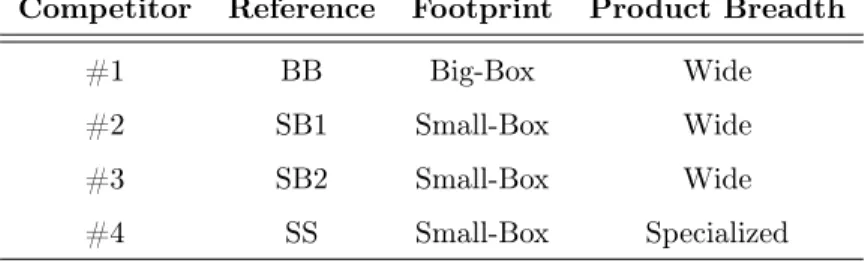
The four competitors (see Table 2) vary in both size and product breadth. Competitor #1 is a big box store with a wide product variety (BB). The remaining three competitors are small-box stores. Competitor #2 and competitor #3 offer a wide assortment of products (SB1 and SB2), whereas competitor #4 specializes in the focal product category for which the limited loyalty program applies (SS). None of these competitors offer a loyalty program similar in structure to that of the focal firm.
7This loyalty program structure is consistent with that of a "customer-tier" LP, as opposed to a "frequency-based" LP, following Blattberg (2008).
8This industry is highly concentrated, with the focal firm and the primary big-box competitor capturing about 85% of market share, according to a 2019 industry report by IBISWorld.
Competitor Reference Footprint Product Breadth
#1 BB Big-Box Wide
#2 SB1 Small-Box Wide
#3 SB2 Small-Box Wide
#4 SS Small-Box Specialized Table 2: Competitor Types
The variety in the size and product breadth allows us to compare how the impact of the compet-itive structure might be competitor or type specific. More importantly, it allows us to gain insight into the extent of category-level versus store-level business stealing.
The latitude and longitude locations of each competitor are collected from the Google Maps API. We first pulled all competitors within a 50 kilometer radius of each of the focal stores, and then pulled all competitors within 50 kilometers of each customer located within a 50 kilometer mile radius of each focal store.9 This expanded footprint ensures that our definition of the competitive
structure is customer centric rather than limited to the perspective of the focal store.
2.3
Quantifying the Competitive Structure
Our analysis measures and highlights the impact of the complex spatial relationship between the customer, the focal store, and the competitors on customer behavior and ultimately firm profits. Quantifying this relationship in such a way to accurately reflect the tradeoffs that an individual likely encounters when deciding which store to visit requires several complex considerations.
A common approach in quantifying competitive structure is to simply use the distance between a focal store and the customer along with the distance between the competitor and the focal store (or more commonly still, an indicator variable if they are both within, say, a 5 kilometer radius of the focal store). The drawback of this approach is that it does not jointly consider the customer-store-competitor location, resulting in a potential homogenization of very distinct competitive structures. This limitation is illustrated in Figure 1: three competitors,C1,C2, andC3, and a customer,I,
9We selected 50 kilometers because this was the maximum radius allowed by the Google Maps API at the time of pulling this information and exceeds the average distance traveled by household by a factor of about 7.
are positioned near the focal storeS. BothC1andC2are nearly the same distance to the store, but
their respective relationships to the customer and the focal store are considerably different. The customer has to pass by the focal store in order to visit the first competitor, C1, which suggests
some spatial advantage for the focal store. However, the second competitor,C2 is positioned right
next to the customer, acting as a convenient alternative to the focal store. In a different case,C2
and C3 are both equidistant to the customer but one is between the customer and the store and
the other is in the opposite direction. One goal of this analysis is to incorporate these complex spatial structures into the manager decision process, a strategy that has heretofore been ignored in the analyses of loyalty program effectiveness.
fi S C1 C2 I C3
Figure 1: Limitation of Radii Approach
We recognize that it is unreasonable to expect a single metric to capture the complex nature of the spatial relationship between the customer, focal store, and competitor in its entirety. Instead, we approach the problem by proposing a large number of metrics, each of which captures at least some of the complex spatial relationship on its own, and then in our empirical analysis uncover which metrics or which interactions between metrics best predict customer behavior. By honing in on the right combination of distance metrics we can determine whichspecificfeatures of the spatial relationship influence customer behavior the most.
We therefore consider standard distance metrics between each customer and competitor with the the focal firm in addition to the following:
• How much closer is the focal store to the customer, relative to the competitor? • Howsparse is the focal store and competitor, relative to the customer?
• Are the focal store and competitor in the same direction from the customer, and to what extent?
We also allow for interactions between population density and distance metrics to incorporate the difference in transportation costs between urban and rural areas. For brevity, the complete description of the distance metrics considered are contained in the appendix.
3
Spatial Competitive Structure and LP Performance
In this section we take advantage of the unique nature of our data and provide descriptive analysis of how customer behavior interacts with joining a loyalty program. Because we observe sales patterns before and after the customer joins the LP we can measure if this behavior changes and if so, how it changes. These results relate to the extant debates on how and whether LPs are effective at increasing profits.
We then provide model free evidence that the spatial competitive structure are key determinants of LP performance. Our analysis focuses on two metrics of LP effectiveness: the probability that a customer joins the program, and the change in average monthly spend for customers who decide to join. Here and throughout the paper, we use the change in spending net of the LP discounts. For customers who join the LP but do not change shopping patterns, this change is negative by default because of the discounts, and all else equal a positive change for this metric can therefore be taken as strictly beneficial for the retailer. In this section we look at how these metrics relate to the the distance between the customer and the focal store and the four competitor types.
One challenge in analyzing LP effectiveness is that the customer’s decision to join the loyalty program may be related to unobserved heterogeneity. While we observe purchases both before and after each customer joins the LP, which allows us to condition on individual-level time-invariant factors, it is still true that if customers join due to anticipated changes in their level of spending, the observed change in behavior can not all be attributed to the loyalty program. We therefore do not treat all changes in spending or other behavior associated with joining the LP as having been caused by the LP. Instead we provide descriptive results on how behavior changes and note that
those changes in behavior that coincide with joining the LP may be of direct interest even without a purely causal interpretation.
In addition, we treat the location of each customer as essentially exogenous prior to joining the LP, in which case the relative difference in spending across customers with respect to the spatial relationship between the customer, the focal store, and the competition still provide valid comparisons. Finally, we replicate our results using only spending that does not qualify for the LP discounts and is thus less likely to result from selection on unobservables.
Descriptive Analysis:
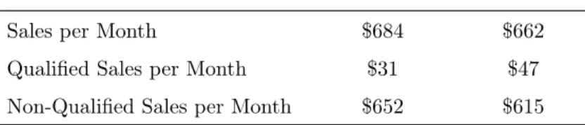
Table 3 first presents the monthly sales at the firm level, split into qualified and non-qualified spend, for all customers and those that enroll in the loyalty program. In terms of overall spending and spending in the LP category, joiners and non-joiners are actually quite similar. As expected, customers who join the loyalty on average have slightly higher monthly spending on products that qualify for the LP discounts but not higher overall spending, and the differences are modest.
All Customers LP Joiners
Sales per Month $684 $662
Qualified Sales per Month $31 $47 Non-Qualified Sales per Month $652 $615
Table 3: Overall Monthly Spending
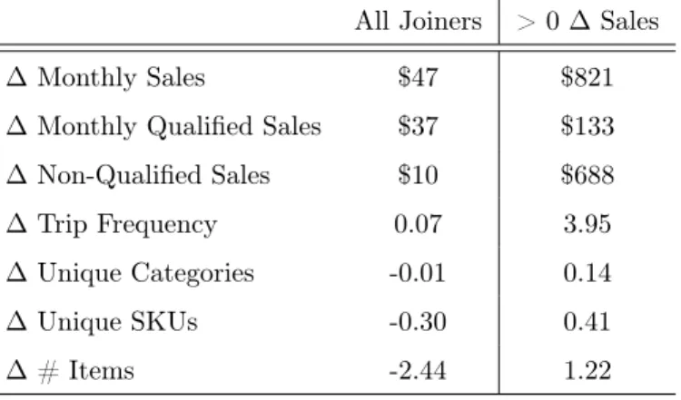
We next show the difference between purchase behavior before and after a customer joins the LP. Table 4 presents the average change in sales, trip frequency, and basket level metrics for customers who join the loyalty program.10 On average, customers tend to increase monthly spending by
about $47 upon joining the loyalty program, with the majority of this change attributed to spend in categories that qualify for LP discounts. This is not surprising, but we also see a positive change in non-qualified spend, which could suggesting that the increase in spending associated with joining the LP spills over into other categories.
Joiners show a small increase in trip frequency, almost no change in number of categories shopped 10For all tables presented in the descriptive analysis, we exclude households that fall within the upper or lower .5% of monthly sales prior to joining the loyalty program to prevent the undue influence of outliers for the summary statistics.
in, and actually slightly decrease the number of unique products purchased. We also note there is substantial heterogeneity across customers.
In the second column, we limit attention to customers whose change in monthly spend was positive. Interestingly, for these customers, the vast majority of the increase is attributed to spend outside of the focal category and does not qualify for the LP discounts. Much of this is driven by a large increase in trip frequency, with more modest changes in basket diversity (distinct categories and SKUs), and basket size. We do not suggest that the LP alone caused all of these changes, but note that within the base of customers that do join the loyalty program, there is substantial heterogeneity in post-join behavior.
All Joiners > 0∆Sales
∆ Monthly Sales $47 $821
∆ Monthly Qualified Sales $37 $133
∆ Non-Qualified Sales $10 $688
∆ Trip Frequency 0.07 3.95
∆ Unique Categories -0.01 0.14
∆ Unique SKUs -0.30 0.41
∆ # Items -2.44 1.22
Table 4: Change in Behavior
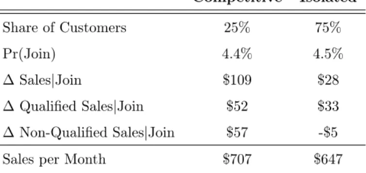
We next consider how a rich but often overlooked source of variation across customers, the competitive structure, can help in attributing the variation in behavior for customers who join the loyalty program. To start, we first label customers as "isolated" if they are located more than eight kilometers (five miles) away from any of the focal store’s competitors and "competitive" otherwise, which indicates there is a competitor relatively close to the customer. We selected this cutoff based on average distance driven by joining customers to surrounding focal stores. Table 5 summarizes a few metrics of interest across these types of customers, namely the probability of joining and the average changes in monthly qualified and non-qualified spend. We also include the average customer sales per month to alleviate concerns that our region labels are associated with substantially different customer types, at least in terms baseline spending patterns.
Approximately one quarter of the customers are located in "competitive" regions and are rela-tively close to one of the four competitors of interest, as identified by the firm providing the data. Relative to customers in more isolated regions, these customers have essentially the same proba-bility of joining the loyalty program but exhibit a substantially larger change in monthly spend. As expected, the change in qualified spend is positive across both groups. However, customers located near the competition also exhibit an equally high change in non-qualified spend. For these customers, joining the loyalty program may present an opportunity to consolidate purchase activity at the focal store. For customers in relatively isolated areas, they are likely devoting most of their budget to the focal store prior to joining the LP and enrollment is unlikely to generate additional spend from competition.
Competitive Isolated Share of Customers 25% 75% Pr(Join) 4.4% 4.5% ∆ Sales|Join $109 $28 ∆ Qualified Sales|Join $52 $33 ∆ Non-Qualified Sales|Join $57 -$5 Sales per Month $707 $647
Table 5: Effect of Competition
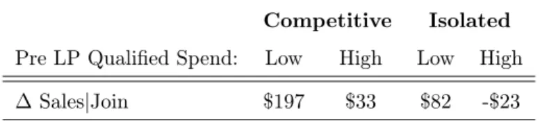
In Table 6 we further split the change in monthly sales based on the median qualified spending amounts prior to joining the loyalty program. In both cases, the larger change in spend comes from below-median spenders pre-LP. This is somewhat counterintuitive since the program targets discounts at high spenders. But most notably, this change is more than twice as large in competitive regions, suggesting that customers with relatively low spend prior to joining are likely splitting their purchase behavior across competitors. For customers with relatively high pre-join spend, the change is not as large, but still higher in the competitive regions. High spenders in isolated markets actually decrease spending somewhat, once discounts are taken into account. This suggests that the degree of competition near a customer can have a substantial impact on customer engagement with the loyalty program.
Competitive Isolated
Pre LP Qualified Spend: Low High Low High
∆ Sales|Join $197 $33 $82 -$23
Table 6: Interaction Between Competition and Pre-Join Spending
To further analyze what is driving these findings we break down the results by competitor type. Figure 2 shows the average change in monthly spending based on the relative isolation of the customer.11 The findings are relatively consistent with the aggregate results, with the exception
of a notably larger increase from customers near the big-box generalist, suggesting this type of competitor presents the most opportunities from which to steal business from, and a notably smaller increase from the small-box specialist, who presents the fewest opportunities from which to steal business from.
To better understand this mechanism, recall that the LP only applies to a specific category, not all products, and that one of the competitors (SS) specializes in selling only that focal category. We thus note the portion of change in spend that occurs in the LP category of interest. Figure 2 highlights this by distinguishing the change in spend as either qualifying for the LP discount (within the focal category) or not, where the combined change is noted by a black square. As expected, a large portion of the change in spend is driven by purchases that qualify for LP discounts. However, there is substantial positive changes outside of the focal category. If there was no spillover effects of the loyalty program, we would expect zero change in purchases that will not impact the LP rewards. Upon joining the LP, customers may decide to consolidate purchase behavior with one store rather than cherry picking rewards from the focal store (in the qualifying category) and continuing with the same purchase patterns at other stores in the non-qualifying categories. For customers located in relatively isolated regions, we see that the gains from focal category purchases tend to be offset by declines in other purchase categories, regardless of competitor type.
Our descriptive evidence suggests that a competitor’s location can have a strong influence on how spending changes when customers join the LP. The analysis motivates the need for a more sophisticated model that captures these complex spatial effects that we present in a later section.
11Note that not all customers may have access to all competitors within a market. Because of these, some customers will not be associated with certain competitors.
0 50 100
All BB SB1 SB2 SS Isolated
Competitor
Change in Monthly Sales|Joining LP ($)
Purchase Cat.
LP Qualified LP Excluded
Figure 2: Change in Monthly Spend by Competitor Type and Purchase Category
Change in Spend Descriptive Analysis:
Before specifying our models of join and spend activity, we first provide a deeper analysis of the change in spend based on pre-join customers characteristics. Ideally, the focal firm would be able to use this information to determine which customers are likely to exhibit the largest change in spend after joining the LP and then target to these customers accordingly.
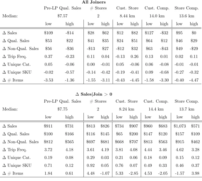
First, Table 7 displays a variety of change metrics based on a median split of five metrics of interest: qualified spending levels prior to joining the LP, number of stores visited, and the three distance metrics of interest: customer-store, customer-competition, and store-competition. We are interested, for instance, in how the firm might predict ex ante what customer characteristics are associated with post-LP increases in spending.
Overall, we see the change in sales is higher for customers 1) with relatively low qualified spend prior to joining the LP, 2) who visit more than two stores pre-join, 3) who are relatively far from the focal store, 4) who are relatively close to the competition, and 5) who shop at stores relatively close to a competitor.
Trip frequency increases substantially more for customers with relatively low qualified sales prior to joining the LP, and for customers who are relatively further from the focal store.
customers with relatively low qualified sales (pre LP), who visit relatively fewer focal stores, and who are relatively close to the competition. Together, these findings continue to suggest that business stealing is more likely for customers with room to grow with the focal firm but also have access to competitors nearby.
Finally, we redo this analysis but focusing on customers who increase spending after joining the loyalty program. The patterns remain relatively consistent but with the magnitudes more pronounced. As in the section with all joiners, the change in spending (in all categories: overall, qualified, and non-qualified) is substantially higher in situations where the customer is close to focal store and the focal store is close to the competition. A similar pattern holds for changes in trip frequency. Interestingly, when the customer is relatively close to the focal store, the changes are lower than those who are relatively far from the focal store.
These initial results begin to illustrate how the competitive structure, defined as the joint re-lationship between the customer, focal store, and competitor locations, are strongly related with a customer’s engagement with the LP. More importantly, we note that the difference between the high and low categories is substantially smaller when the median split is based on pre-join qualified sales or number of stores visits, suggesting that in some cases spatial characteristics appear to be more informative in identifying change in spend versus traditional behavior based metrics.
All Joiners
Pre-LP Qual. Sales # Stores Cust. Store Cust. Comp. Store Comp.
Median: $7.57 2 8.44 km 14.0 km 13.6 km
low high low high low high low high low high
∆Sales $109 -$14 $28 $62 $12 $82 $127 -$32 $95 $0 ∆Qual. Sales $53 $22 $41 $35 $24 $51 $64 $12 $46 $29 ∆Non-Qual. Sales $56 -$36 -$13 $27 -$12 $32 $63 -$43 $49 -$29 ∆Trip Freq. 0.37 -0.23 0.11 0.04 -0.13 0.26 0.13 0.01 0.02 0.11 ∆Unique Cat. 0.05 -0.06 0.00 -0.01 0.05 -0.06 0.06 -0.08 -0.01 -0.01 ∆Unique SKU -0.02 -0.57 -0.14 -0.42 -0.19 -0.41 0.09 -0.68 -0.27 -0.32 ∆# Items -3.53 -1.36 -1.55 -3.11 -0.43 -4.45 -1.58 -3.30 -0.40 -4.47 ∆ Sales|Join > 0
Pre-LP Qual. Sales # Stores Cust. Store Cust. Comp. Store Comp.
Median: $7.75 2 8.24 km 14.4 km 13.7 km
low high low high low high low high low high
∆Sales $911 $731 $813 $826 $734 $907 $960 $683 $1,073 $571 ∆Qual. Sales $100 $166 $116 $145 $65 $200 $147 $120 $157 $109 ∆Non-Qual. Sales $812 $565 $697 $681 $668 $707 $813 $563 $915 $462 ∆Trip Freq. 3.72 4.18 3.61 4.19 3.81 4.08 4.44 3.46 4.62 3.28 ∆Unique Cat. 0.19 0.08 0.29 0.03 0.21 0.06 0.18 0.09 0.15 0.12 ∆Unique SKU 0.71 0.12 0.92 0.05 0.76 0.07 0.49 0.33 0.46 0.37 ∆# Items 1.84 0.61 4.48 -1.07 5.33 -2.85 4.53 -2.05 -1.57 3.98
Table 7: Change in Behavior Based on Pre-Join Characteristics
Patterns Among Profitable Joiners: Within the customers who increase spending upon joining the LP, we investigate other changes in behavior to determine if there are patterns as to what is driving the positive change in spend. We focus on using the non-spatial variables to see if we might identify segments to provide insight into specifically how engagement with the LP changes upon joining.
In Table 8 we provide a cross-tabulation of selected measures of shopping behavior for these customers. The cells indicate the proportion of customers that fall into each quadrant. We construct the quadrants based on whether there is a substantial increase (which we define as at least a 15% increase in the metric) or if the behavior is flat or even decreasing. For example, of the customers with a positive change in spend, 13.9% of them showed no appreciable increase in trip frequency paired with a significant increase basket size. Within each cell we also note the average increase in spending upon joining to highlight the heterogeneity across customers and relative value of each segment.
As expected, most consumers show an increase in the given variables, since we are selecting only customers who increase spending overall. Of greater interest are the customers who land in the off-diagonal groups - that is, customers who exhibit a positive change in one metric at the expense of a negative change in another. In the complementary Table 9 we provide additional information about the customers within these off-diagonal cells, namely their pre-join behavior and simple spatial metrics.
The first cross tabulation shows that more than one third of those who increase spending do so via increased trip frequency but with no increase in per-trip basket size. This behavior is consistent with consolidating purchases from multiple competing stores to only the focal store after joining the LP and we refer to this group asconsolidators. The average change in spend of this group at $749 is nearly twice that of the complementary group, who increase basket size but not trip frequency. This is despite the fact that in the complementary table these customers (in the "lower left" cell) have similar pre-join spending levels as those in the opposite cell ("top right"). The spatial information provides some indication of why these customers may have proven to be so valuable. The more valuable group is actually further away from the focal stores, at a distance of more than 10km versus about 8km, and on average but essentially the same distance to the competition. That is, it appears that after joining the customers shift trips that occur elsewhere to the focal store.
The middle cross-tabulation compares changes in number of items purchased and the average price per item. The largest group increases spending by buying more items but without a substantial increase in average price. But about 31% of customers show no increase in basket size but a substantial increase in the price paid per item, suggesting that these customers may be responding to the LP discounts either by upgrading to more expensive items after joining the LP or shifting higher purchases away from competitor stores. We refer to this group asupgraders. These customers
also increase their total spending by more than twice as much as those who simply buy more items. We see a similar pattern as the first section: the customers in the more valuable off-diagonal cell (in terms of change in spend after joining) are relatively further away from the focal store. Again, customers that join but are close to the focal store are likely devoting most of their budget to the focal store as is, so joining is unlikely to have a pronounced impact on spend (along with other metrics) unless there is a competitor from which to take business from. The upgraders are also higher spenders pre-join, suggesting they are more likely to receive the LP discounts.
Finally, the bottom cross-tabulation shows again that close to a third of customers have no increase in qualified sales but a substantial increase in non-qualified sales. In terms of change in spend upon joining, those in the top right cell are more than five times more valuable than those in the lower left cell, even though the pre-join sales per month are actually lower. This behavior is again consistent with being a consolidator, shifting non-qualified spending in response to joining the LP. As with before, the spatial metrics provide additional insight into why we might see a marked increase in non-qualified sales: they are more than 2km closer to a competitor, on average, and the focal store is about 1km closer to a competitor, on average.
Our deep analysis of the joining customers continues to provide insight on how behavior changes upon joining the LP and illustrate that spatial metrics provide incremental value in identifying valuable customer groups. In these tables, many of the behavior-based metrics are nearly identical, so any effort to pinpoint the valuable customers based on behavior based metrics alone may be difficult. However, we have provided preliminary evidence that spatial metrics appear to indicate which customers are valuable, both in aggregate analyses as shown earlier and in very detailed analyses shown in this section.
In the next section, we integrate spatial metrics into predictive models of customer behavior. In addition to the relatively simple spatial metrics already presented in the descriptive analysis, we consider a variety of other subtle spatial metrics which may also influence probabilities of joining the loyalty program and change in spend behavior.
∆Basket Size (# Items) Flat/Decrease Sig. Increase
∆ Trip Frequency Flat/Decrease 14.4% 13.9%
$814 $312
Sig. Increase 35.8% 35.8% $749 $1,094
∆Price/Item
Flat/Decrease Sig. Increase
∆ Basket Size (# Items) Flat/Decrease 19.4% 30.8% $233 $1,103 Sig. Increase 34.3% 15.4% $591 $1,506
∆ Non-Qualified Sales Flat/Decrease Sig. Increase
∆ Qualified Sales Flat/Decrease 4.0% 27.9%
$59 $636
Sig. Increase 12.4% 55.7% $115 $1,125 Table 8: Positive∆ Sales|Join Proportions and∆ Sales
1: Trip Freq v. # Items 2: # Items v. Price/Item 3: Qual v. Non-Qual Sales Pre LP Metrics Top Right Lower Left Top Right Lower Left Top Right Lower Left
Sales per Month $506 $464 $604 $414 $448 $581
Non-Qual Sales/Month $471 $442 $577 $388 $410 $543 Qual Sales/Month $35 $22 $27 $26 $38 $38 Trips/Month 6.66 4.36 5.33 4.97 5.32 6.07 Unique Categories 1.73 2.06 2.08 1.86 2.08 1.90 Unique SKUs 3.12 4.10 4.17 3.49 4.02 3.80 Basket Size 6.42 18.32 18.50 7.32 9.48 11.23 Price/Item $17.86 $10.72 $9.88 $19.82 $11.34 $13.36 Stores Visited 1.96 2.29 2.21 2.06 2.04 2.44 Store-Customer km 8.24 10.06 9.46 8.40 9.27 9.98 Cust.-Competitor km 15.71 16.13 15.79 13.75 14.34 16.44 Store-Competitor km 14.59 14.18 14.02 13.51 14.20 15.14
Table 9: Quadrants of Interest for Positive∆ Sales|Join
4
LASSO Regularization and Competitive Targeting
In this section we propose and estimate a predictive model of how customer behavior changes after joining the LP. This model takes as inputs detailed data on pre-join spending patterns as well as complex representations of the spatial relationships between customers and their local competitive structures. We broadly define these data on spending patterns as capturingvertical quality or the value of a customer in terms of their overall demand, and define the data on local competitive structures as capturinghorizontal quality or how likely it is to shift a customers spending from a competitor’s store to the focal store. Because spending at competitors is unobserved spatial data must fill this role. Estimating a model with these two inputs serves two purposes. First, we can analyze the estimation results directly to compare the relative predictive power of our complex competitive structure (horizontal) variables and traditional predictors of LP effectiveness like sales history (vertical) variables, as well as simple rule-of-thumb variables or simple measures of customer
location. This relative predictive power is informative on how LPs manage to increase spending, i.e., via demand expansion or business stealing.
Second, the estimation suggests a hypothetical targeting strategy for a firm seeking to improve LP effectiveness by providing predictions of which customers are the most profitable to target based on their spending histories, precise locations, and unique competitive structures. The wide variation across customers in profitability suggests the gains from targeting the program can be quite large and spatial data on customer location may be more accessible than historical sales data in addition to having strong predictive power.
We estimate the impact of the competitive structure on customer behavior with two models. We first model the change in spending conditional on participating in the LP and the competitive structure. Next, we model the the probability that a customer joins the firm’s loyalty program, con-ditional on the competitive structure. We estimate separately to allow these variables to influence the changes in spend and join probabilities differently.
The goal of the estimation is to predict which customers are likely to increase net spending as members of the LP based on their past sales and spatial characteristics. Because the goal is prediction and the data are high-dimensional, the problem is well-suited to statistical methods built around dimension reduction or “regularization.” We ultimately use a LASSO approach because this will allow us to test inclusion of a large number of possible spatial measures and let the model select the most predictive variables. The output also provides a clearer interpretation than other methods and one goal of the analysis is to assess which individual factors best predict LP effectiveness. Finally, the results can be used to assess whether the vertical measures representing spending-based customer value or the horizontal variables representing location-spending-based customer vulnerability to competitors are more effective at predicting behavior. In our discussion of the results we show how this comparison is informative of how and when quantity discounts or behavior-based pricing schemes are likely to succeed.
4.1
Change in Spend
We first estimate the change in monthly store-level spend, conditional on joining the loyalty pro-gram. Letyis be thechange in monthly sales for customeriat stores. We model this relationship as:
yis=β′Xis+δ′Zis+εis (1)
where εis is an unobserved, normally distributed random error centered at zero. Here Xis
contains the competitive structure parameters between customer i at focal store location s and
Z contains firm-level marketing and store-specific customer purchase behavior. These metrics are intended to jointly capture the complex spatial relationships between the customer, focal store, and competitors. Since there can be more than one focal store in the vicinity of an individual, these metrics vary across each storesfor a given individuali. Likewise, since each customer’s location is unique, the spatial metrics also vary across each individualifrom all observations for stores.
β reflects the impact of the competitive structure on an individual’s likelihood of joining the program. We avoid specific interpretations within this vector of coefficients (e.g. representing the cost of transportation) and instead interpret the coefficients as holistically capturing the many spatial factors that a customer considers before committing to the firm’s loyalty program (e.g., convenience of the focal store relative to the competition, isolation of the focal store, distance to the store versus other competitors, etc.).12
Zis includes traditional recency, frequency, and monetary value (RFM) variables along with basket specific metrics: monthly trip frequency, overall sales, distinct number of items, number of product categories, basket size, discounts received, sales in the category of interest, and sales in the category of interest for those products that are included in the limited LP. We also include the proportion of sales in the category of interest, an indicator for whether the customer received marketing activity specifically encouraging joining the LP, and an indicator for whether the customer received any marketing promotion.
δ captures the effects of the marketing and past purchase behavior on the change in monthly spend. For instance, customers with relatively low trip frequencies may be associated with greater changes in monthly spend due to trip consolidation.
12We recognize that self-selection could potentially lead to biased estimates of change-in-spend parameters since customers choose to enroll into the loyalty program. While this does not effect the predictive power of the model or our ability to compare the relative importance of different data types in contributing to this predictive power, it may effect the direct interpretation of coefficients. We mainly refrain from interpreting these directly, but in addition, to mitigate these concerns, we estimated a Heckman-style two-stage correction method with a flexible control function in an attempt to correct any remaining selection bias. The results suggested that self-selection is inconsequential and the coefficients estimates of interest were nearly identical to what we present in this paper. The full results of this are available in the Appendix. See Heckman (1979) for an introduction to the two-stage estimator and Ahn and Powell (1993) for extensions to more flexible selection correction functions.
4.2
Join Rate
We next estimate the probability that a given customer joins the LP. Having customers enroll in the LP may be of direct interest to the firm regardless of changes in spending that occur due to joining if, for instance, this allows the firm to target future marketing at the customer or use their data for other purposes. Let the indirect utility of joining the firm’s loyalty program for customer
iat focal storesbe
uis=γ′Xis+κ′Zis+ηis (2)
Here Xis and andZis are defined in the same way as in the change in spend model. The error termηis captures the idiosyncratic variation in utility across customers and stores. Assuming the
{ηis} are independent and identically distributed Type I extreme value, we can derive the join probabilities as follows:
Pr (ji= 1|Xis, Zis, γ, κ) = exp (γ′Xis+κ′Zis)
1 + exp (γ′Xis+κ′Zis) (3)
whereji= 1if customerijoins the limited loyalty program at some point during the observed data.
4.3
LASSO Estimation
Our proposed model contains a large number of spatial variables defined to capture the competitive structure. On the one hand, capturing the spatial relationship between the customer, focal store, and competitors is complex and may require many variables. However, all else being equal a concise model is preferable from a managerial standpoint. In addition, many of the spatial metrics we devised may be redundant or highly correlated with each other. To systematically remove variables that are either unnecessary or redundant we employ the Least Absolute Shrinkage and Selection Operator (LASSO) estimator, introduced by Frank and Friedman (1993) and Tibshirani (1996).
In general, for a model with a k-dimensional parameter vectorθ the LASSO method performs the following: (θ∗) = arg min ( −logL(θ) +λX k |θk| ) (4)
WhereL is the likelihood of data given the model specified, and λis a tuning parameter that represents the penalty incurred if we choose a nonzero value for any parameterθk. This approach regulates the trade-off between an accurate model with more predictive power and a concise model that is more readily interpretable by managers.13 We select the tuning parameter λthrough ten
fold cross-validation, which is perhaps the simplest and most widely used method for this task.14
4.4
Estimation Results
The results from the LASSO estimation are presented in Table 10. For model validation purposes, we split the original data into a 75% training set and 25% test set. The results presented below were estimated using the training set alone. For brevity, the table only displays variables that are significant in at least one of the two models. First we discuss how the competitive structure influences the join probabilities before discussing the estimated impact on the change in monthly spending, as both are influenced differently. From a statistical standpoint, it is relatively easy to interpret the marginal effects of each the variables. However, we must emphasize that many of the spatial impacts are codependent and interpreting the marginal effect of one coefficient while holding another spatial variable constant is sometimes impossible. Later, we present stylized visual representations to better understand the impact of the spatial relationships on change in spend.
4.4.1 Join Probabilities
The LASSO estimation results are shown in Table 10, and the full list of spatial variable definitions is provided in Table 14. In this join model many of the traditional distance metrics drop out of the model (e.g., direct distance between the focal store and the customer) in favor of secondary spatial metrics.
For instance, as the angle between the big box competitor (BB) increases, the probability of joining the LP at the focal store also increases. This indicates that the probability of joining increases if the competitor is in the opposite direction relative to the customer, rather than in the 13An alternative approach would be a ridge regression or similar method. In this case the penalty is applied more smoothly, shrinking coefficients on highly correlated variables towards each other. We prefer the LASSO approach because the penalty structure removes coefficients entirely, resulting in clearer model interpretation. Specifically, we can see that many non-spatial variables will drop out altogether. This result is a notable output of interest. A ridge regression would lack this clean interpretation but would result in similar quantitative predictions and can be provided upon request.
same direction. This effect also holds for the small box specialist (SS).
The last two sets of spatial components (ccbar and icbar) are designed to account for differences in markets with the presence of multiple competitors of the same type. The first of these variables, ccbar, is the average distance between each competitor and its competitive center (defined as the average latitude and longitude across competitors of the same type). A relatively high value indicates that the competitors are relatively spread out in a market. The negative coefficient on the big box generalist (ccbar_1) indicates that the more dispersed these stores are in a market, the less likely the customer is to join the LP. The second variable, icbar, measures the average distance between each customer and each of the competitors. While a customer may be close to the competitive center, a high value of icbar indicates that each individual competitor (of a given type) is still relatively far away. This coefficient is positive for the two small-box generalists (SB1 and SB2), suggesting that a relatively sparse distribution of these competitors may be beneficial to the focal firm.
Finally, we see a strong positive effect on the proportion of sales in the category of interest: customers who dedicate a greater portion of store spend to the LP category are more likely to benefit from the LP discounts. There is also a positive impact of whether or not they received a marketing promotion, for both general emails and those specifically designed to enroll them in the LP.
4.4.2 Change in Monthly Spend
In this section we now review the importance of competitive structure as a predictor of the estimated LP effectiveness, as measured by change in monthly spending at the focal store, conditional on joining the firm’s loyalty program. Recall the dependent variable in this estimation is the change in monthly spend after joining the loyalty program, net of any LP discounts. For this table, we only included customers who had at least some spending both before and after joining. Since we are interested in how spendingchanges after joining, rather than whether spending occurs or not, this seems to be a reasonable filter.
First, there is a positive impact on the squared distance between the customer and the focal store, suggesting that the greater gains come from those located further away from the focal store. This aligns with our previous intuition: customers located near the focal store are more likely to already dedicate the majority of their spend with the focal store, so the potential for increases in
spend are limited, relative to those who are further away and thus more likely to be sharing spend with the competition.
Importantly, the distance between the customer and the competition also influences changes in spend at the focal store. Customers who exhibit the largest changes in spend are those who are relatively far from the the big-box generalist (ic1sq) and the second small-box generalist (ic3sq) and close to from the other competitors, holding all other variables constant.
Many of the radius band coefficients drop out of this model. However, we see that the intercept angle is retained. The difference in the estimated change in spend for a customer where a big-box (BB) competitor is in the same line of travel as the focal store (intercept angle of zero) versus in the opposite direction (intercept angle of 180 degrees) is about $124, holding all other variables constant. This is a non-trivial amount that cannot be captured using traditional spatial measures. However, it is important to again point out that many of these distance metrics cannot vary independently of others. The visual results presented later will illustrate the degree to which the intercept angle influences the change in spend while simultaneously accounting for other changes.
Finally, population density along with its interactions with the direct distance measures has a significant impact on the change in monthly spend. On its own, the effect is positive: more densely populated areas are associated with a greater change in spend. This is intuitive as more densely populated areas tend to have a greater level of competition and higher incomes. There are also numerous interactions with our simple distance metrics. For instance, increases in the distance between the store and the customer influence customers in dense areas more negatively, relative to customers in less dense areas. This appears to be capturing the challenges of traveling in more densely populated areas (e.g., traveling a given distance in a city versus a rural setting).
As an important robustness check, we also include a column where the estimation proceeds as before but only using the change in spending on products that do not qualify for the LP discounts. Comparing this column and the column for all spending shows a very high correlation in the LASSO coefficients and perfect correlation in which variables are retained.
4.4.3 Summary
The LASSO results suggest that the customer behavior appears to be strongly influenced by the competitive structure of the local market. The regularization tends to keep quite a few of the spatial metrics, suggesting that relatively simple distance metrics are, on their own, unable to fully
characterize the predicted behavior. This is not very surprising: there are many intuitive reasons why a customer may change their spending patterns after joining a loyalty program with respect to their location.
4.5
Visual Representation of Results
Even after variable reduction via LASSO, it is still difficult to interpret how the competitive struc-ture influences estimated changes in spend due to the codependency between variables. We therefore visually illustrate the LASSO’s results on how the competitive structure influences LP effectiveness. For brevity, we limit our discussion to two heatmaps that show the predicted change in spending for hypothetical customers. Additional heatmaps are provided in the Appendix. These maps show how there is large heterogeneity across different customers with different competitive structures in the potential gains from having them join the LP. However, since these maps are mostly stylized representations of the actual data we focus on comparing the magnitudes across maps rather than specific prediction levels.
Figure 3 plots all four competitors, each an equal distance from the focal store. The color on the heatmap reflects the estimated change in spend from a customer in that position if they were to join the focal store’s loyalty program, with shades closer to white representing greater increases. This map shows that most of the gains are from customers near the big-box generalist, and less so from the small-box specialist. This map highlights that the value of a potential customer is heavily dependent on the extent to which the focal store can steal business from the competition. This also represents visually how a targeting strategy might be employed using complex representations of spatial relationships constructed from readily available data, even in the absence of past sales data on customers.
Table 10: Lasso Pr(Join) and Change in Sales|Join
Coefficient Pr(Join) Change in Sales|Join Change in Non-Qualified Sales|Join
1 (Intercept) -3.5018 -27.9689 -46.4571 2 sisq 0.0194 0.0280 3 ic2 0.0010 4 ic3 0.0054 5 ic1sq 0.2158 0.2088 6 ic2sq -0.1387 -0.1415 7 ic3sq 0.1429 0.1315 8 ic4sq -0.0001 -0.1381 -0.1043 9 sc1 0.0026 10 sc1sq 0.0001 -0.0308 -0.0322 11 sc2sq -0.0615 -0.0375 12 sc3sq -0.0950 -0.1016 13 sc4sq -0.0001 0.1128 0.0874 14 s4 -0.3020 15 nAll_1 0.0225 16 n1_1 0.6830 17 n3_1 0.1946 18 n5_1 0.1593 19 n10_1 -0.0474 20 n15_1 0.0514 21 nAll_2 -0.0014 0.4183 0.3750 22 n1_2 -0.2532 23 n10_2 0.0332 24 n15_2 -0.0158 25 nAll_3 -0.0141 26 n1_3 0.2901 27 n3_3 -0.0033 28 n5_3 -0.0690 29 n10_3 0.0579 30 nAll_4 -0.0077 31 n3_4 0.1371 32 n15_4 -0.0044
33 cInt1: BB intercept angle 0.0013 0.6900 0.7909
34 cInt2: SB1 intercept angle -0.0945 -0.1817
35 cInt3: SB2 intercept angle 0.0005 0.5190 0.5555
36 ccbar_1 (avg. BB-BB comp. center km) -0.0126
37 ccbar_2 (avg. SB1-SB1 comp. center km) 0.0097 0.4599 0.5875
38 icbar_2 (avg. customer-SB1 km) 0.0036
39 icbar_3 (avg. customer-SB2 km) 0.0039
40 icbar_4 (avg. customer-SS km) -0.0001
41 Prop. of sales in LP category (pre LP) 5.7842
42 Received promotional email 0.0762
43 Received promotional email for LP 1.3227
44 Trips/month (pre LP) 0.0106 -24.5945 -24.1253
45 Total sales (pre LP) 0.0002 0.0037 0.0002
46 Total sales in LP category (pre LP) 0.1177 0.1106
47 Total qualified sales in LP category (pre LP) -0.1678 -0.1058
48 Number of focal stores w/i 60km 0.0035 1.0196 1.0950
49 Population Density (in sq miles) 0.0290 0.0262
50 Population Density x si -0.0016 -0.0016
51 Population Density x ic1 -0.0023 -0.0021
52 Population Density x ic2 -0.0007 -0.0011
53 Population Density x ic3 -0.0003 -0.0002
54 Population Density x ic4 0.0043 0.0043
55 Population Density x sc1 0.0001 56 Population Density x sc2 0.0014 0.0012 57 Population Density x sc3 -0.0007 58 Population Density x sc4 -0.0026 -0.0028 59 distinctSKU -0.0055 60 numItems 0.0019 -4.1178 -3.6378 61 distinctCategories -0.0989
● ● ● ● ● ● ● ● ● ● ● ● ● ● ● ● ● ● ● ● ● ● ● ● ● ● ● ● ● ● ● ● ● ● ● ● ● ● ● ● ● ● ● ● ● ● ● ● ● ● ● ● ● ● ● ● ● ● ● ● ● ● ● ● ● ● ● ● ● ● ● ● ● ● ● ● ● ● ● ● ● ● ● ● ● ● ● ● ● ● ● ● ● ● ● ● ● ● ● ● ● ● ● ● ● ● ● ● ● ● ● ● ● ● ● ● ● ● ● ● ● ● ● ● ● ● ● ● ● ● ● ● ● ● ● ● ● ● ● ● ● ● ● ● ● ● ● ● ● ● ● ● ● ● ● ● ● ● ● ● ● ● ● ● ● ● ● ● ● ● ● ● ● ● ● ● ● ● ● ● ● ● ● ● ● ● ● ● ● ● ● ● ● ● ● ● ● ● ● ● ● ● ● ● ● ● ● ● ● ● ● ● ● ● ● ● ● ● ● ● ● ● ● ● ● ● ● ● ● ● ● ● ● ● ● ● ● ● ● ● ● ● ● ● ● ● ● ● ● ● ● ● ● ● ● ● ● ● ● ● ● ● ● ● ● ● ● ● ● ● ● ● ● ● ● ● ● ● ● ● ● ● ● ● ● ● ● ● ● ● ● ● ● ● ● ● ● ● ● ● ● ● ● ● ● ● ● ● ● ● ● ● ● ● ● ● ● ● ● ● ● ● ● ● ● ● ● ● ● ● ● ● ● ● ● ● ● ● ● ● ● ● ● ● ● ● ● ● ● ● ● ● ● ● ● ● ● ● ● ● ● ● ● ● ● ● ● ● ● ● ● ● ● ● ● ● ● ● ● ● ● ● ● ● ● ● ● ● ● ● ● ● ● ● ● ● ● ● ● ● ● ● ● ● ● ● ● ● ● ● ● ● ● ● ● ● ● ● ● ● ● ● ● ● ● ● ● ● ● ● ● ● ● ● ● ● ● ● ● ● ● ● ● ● ● ● ● ● ● ● ● ● ● ● ● ● ● ● ● ● ● ● ● ● ● ● ● ● ● ● ● ● ● ● ● ● ● ● ● ● ● ● ● ● ● ● ● ● ● ● ● ● ● ● ● ● ● ● ● ● ● ● ● ● ● ● ● ● ● ● ● ● ● ● ● ● ● ● ● ● ● ● ● ● ● ● ● ● ● ● ● ● ● ● ● ● ● ● ● ● ● ● ● ● ● ● ● ● ● ● ● ● ● ● ● ● ● ● ● ● ● ● ● ● ● ● ● ● ● ● ● ● ● ● ● ● ● ● ● ● ● ● ● ● ● ● ● ● ● ● ● ● ● ● ● ● ● ● ● ● ● ● ● ● ● ● ● ● ● ● ● ● ● ● ● ● ● ● ● ● ● ● ● ● ● ● ● ● ● ● ● ● ● ● ● ● ● ● ● ● ● ● ● ● ● ● ● ● ● ● ● ● ● ● ● ● ● ● ● ● ● ● ● ● ● ● ● ● ● ● ● ● ● ● ● ● ● ● ● ● ● ● ● ● ● ● ● ● ● ● ● ● ● ● ● ● ● ● ● ● ● ● ● ● ● ● ● ● ● ● ● ● ● ● ● ● ● ● ● ● ● ● ● ● ● ● ● ● ● ● ● ● ● ● ● ● ● ● ● ● ● ● ● ● ● ● ● ● ● ● ● ● ● ● ● ● ● ● ● ● ● ● ● ● ● ● ● ● ● ● ● ● ● ● ● ● ● ● ● ● ● ● ● ● ● ● ● ● ● ● ● ● ● ● ● ● ● ● ● ● ● ● ● ● ● ● ● ● ● ● ● ● ● ● ● ● ● ● ● ● ● ● ● ● ● ● ● ● ● ● ● ● ● ● ● ● ● ● ● ● ● ● ● ● ● ● ● ● ● ● ● ● ● ● ● ● ● ● ● ● ● ● ● ● ● ● ● ● ● ● ● ● ● ● ● ● ● ● ● ● ● ● ● ● ● ● ● ● ● ● ● ● ● ● ● ● ● ● ● ● ● ● ● ● ● ● ● ● ● ● ● ● ● ● ● ● ● ● ● ● ● ● ● ● ● ● ● ● ● ● ● ● ● ● ● ● ● ● ● ● ● ● ● ● ● ● ● ● ● ● ● ● ● ● ● ● ● ● ● ● ● ● ● ● ● ● ● ● ● ● ● ● ● ● ● ● ● ● ● ● ● ● ● ● ● ● ● ● ● ● ● ● ● ● ● ● ● ● ● ● ● ● ● ● ● ● ● ● ● ● ● ● ● ● ● ● ● ● ● ● ● ● ● ● ● ● ● ● ● ● ● ● ● ● ● ● ● ● ● ● ● ● ● ● ● ● ● ● ● ● ● ● ● ● ● ● ● ● ● ●