Short-Term Wind Power Prediction Using a Wavelet Support Vector Machine

(1)

DigitalCommons@University of Nebraska - Lincoln

Faculty Publications from the Department of

Electrical and Computer Engineering

Electrical & Computer Engineering, Department

of

4-2012

Short-Term Wind Power Prediction Using a Wavelet Support

Vector Machine

Jianwu Zeng

University of Nebraska–Lincoln, [email protected]

Wei Qiao

University of Nebraska–Lincoln, [email protected]

Follow this and additional works at: https://digitalcommons.unl.edu/electricalengineeringfacpub

Part of the Electrical and Computer Engineering Commons

Zeng, Jianwu and Qiao, Wei, "Short-Term Wind Power Prediction Using a Wavelet Support Vector

Machine" (2012). Faculty Publications from the Department of Electrical and Computer Engineering. 195.

https://digitalcommons.unl.edu/electricalengineeringfacpub/195

This Article is brought to you for free and open access by the Electrical & Computer Engineering, Department of at DigitalCommons@University of Nebraska - Lincoln. It has been accepted for inclusion in Faculty Publications from the Department of Electrical and Computer Engineering by an authorized administrator of

(2)

IEEE TRANSACTIONS ON SUSTAINABLE ENERGY, VOL. 3, NO. 2, APRIL 2012 255

Short-Term Wind Power Prediction Using a Wavelet

Support Vector Machine

Jianwu Zeng

, Student Member, IEEE

, and Wei Qiao

, Member, IEEE

Abstract—This paper proposes a wavelet support vector

ma-chine (WSVM)-based model for short-term wind power prediction (WPP). A new wavelet kernel is proposed to improve the general-ization ability of the support vector machine (SVM). The proposed kernel has such a general characteristic that some commonly used kernels are its special cases. Simulation studies are carried to validate the proposed model with different prediction schemes by using the data obtained from the National Renewable Energy Laboratory (NREL). Results show that the proposed model with a

fixed-step prediction scheme is preferable for short-term WPP in terms of prediction accuracy and computational cost. Moreover, the proposed model is compared with the persistence model and the SVM model with radial basis function (RBF) kernels. Results show that the proposed model not only significantly outperforms the persistence model but is also better than the RBF-SVM in terms of prediction accuracy.

Index Terms—Radial basis function (RBF), sigmoid function,

support vector machine (SVM), wavelet, wind power prediction (WPP).

I. INTRODUCTION

W

IND energy, as a clean and renewable energy source, has received more and more attention in the last decade [1]–[6]. However, due to the intermittency of a wind energy source, the increasing penetration of wind power can create sig-nificant uncertainties in electricity generation, which has an ad-verse effect on power system operation. To avoid or mitigate the adverse effect of integrating wind power, it is essential to de-velop methods for wind power prediction (WPP). WPP is a tech-nique which provides information on how much wind power can be expected at a given point in time [8]. A good short-term WPP will help achieve grid stability and a favorable trading perfor-mance on the electricity markets [9].

The existing WPP models can be generally classified into two categories: physical models and statistical models. The physical models [10] take as input not only historical data on wind power but also meteorological information obtained from numerical

Manuscript received February 28, 2011; revised November 02, 2011; accepted December 04, 2011. Date of current version March 21, 2012. This material is based upon work supported by the National Science Foundation under CAREER Award ECCS-0954938 and the Federal Highway Adminis-tration under Agreement DTFH61-10-H-00003. Any opinions,findings, and conclusions or recommendations expressed in this publication are those of the authors and do not necessarily reflect the view of the National Science Foundation or Federal Highway Administration.

The authors are with the Department of Electrical Engineering, University of Nebraska-Lincoln, Lincoln, NE 68588-0511 USA (e-mail: [email protected]. edu; [email protected]).

Color versions of one or more of thefigures in this paper are available online at http://ieeexplore.ieee.org.

Digital Object Identifier 10.1109/TSTE.2011.2180029

weather prediction (NWP) and other information, such as local weather conditions [11]–[13]. The statistical models [14], [15] predict wind power by using only measured historical and cur-rent values of wind power. No extra information is required. Compared to the statistical models, the physical models usually perform well for longer-term prediction (e.g., more than 6 hours ahead) but are more complicated and require vast computational resources. The statistical models are preferable for short-term prediction [16]. By combining the physical models and statis-tical models, some hybrid-model-based tools [17] were devel-oped, which incorporate the benefits of both models to improve the performance of WPP [8]. This paper focuses on the statis-tical model-based short-term WPP.

The statistical models can be further divided into linear and nonlinear models. The persistence model and autoregressive moving average (ARMA) model are two traditional linear models used in WPP [18]. The commonly used nonlinear statis-tical WPP models are based on artificial intelligence techniques, such as artificial neural networks (ANNs) [19]–[21] and support vector machines (SVMs) [22]. Nonlinear models were proven to more accurately capture the effects of nonstationary wind characteristics than linear models [20], [21]. Recent results have shown that SVM-based models either compare favorably with [21] or outperform [9] the ANN-based models in WPP. For example, SVM-based models have been found to take less computational time compared to ANN-based models [23].

Wavelet analysis is a relatively new mathematical technique used to analyze the nature of signals. This technique has been recognized as a promising tool for nonstationary signal approx-imation and frequency analysis. In [24], the original wind speed series was decomposed with wavelets. The ARMA model was then used to predict the coefficients of different layers of the wavelets, which outperformed the method of using the ARMA model directly to predict wind speed. De Aquino [25] used wavelet transform as a data preprocessing technique for an ANN for WPP, which is superior to the model using ANN only. In [25], the inputs to the ANN are the wavelet coefficients derived from the multiresolution analysis [26].

This paper proposes a statistical WPP model which combines wavelet analysis with SVM. A new SVM kernel is proposed based on the wavelet mother function in [27]. The new kernel can change between a radial basis function (RBF) kernel and a Mexhat kernel and outperforms the RBF as well as the Mexhat kernels. The resulting wavelet SVM (WSVM)-based model is preferable for short-term WPP. The proposed model is validated by using data obtained from the National Renewable Energy Laboratory (NERL) and is compared with the persistence model and RBF-SVM model to show its superiority.

(3)

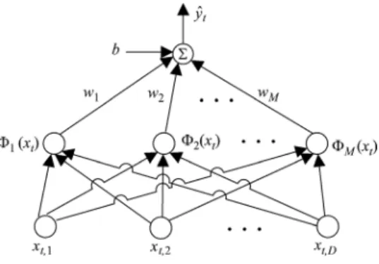
Fig. 1. Structure of an SVM.

II. WAVELETSUPPORTVECTORMACHINE

SVM belongs to the class of kernel methods. The use of SVM for time series prediction can be expressed as follows:

(1) where is the predicted value of the time series;

is the input regression vector consisting of historical data of the time series and ;

is a bias term; is the weight vector; and is a nonlinear feature map, which trans-forms the input vector to a higher-dimensional vector . Fig. 1 shows the structure of an SVM, where and denote the th and th element of and , respectively.

In an SVM, the historical data of the time series is mapped into a higher-dimensional feature space via nonlinear mapping . Then linear regression is used in the high-dimensional feature space to train SVM and to predict the time series, which is equivalent to solving a nonlinear regression problem in the low-dimensional space of the original time series [22]. The key issue to solving such a prediction problem is tofind the optimal values of the SVM parameters and . This can be done by solving a constrained optimization problem. According to the objective function of the optimization problem, the SVMs can be divided into the least-square SVM (LS-SVM) and -SVM.

A. Least-Square Support Vector Machine

In the LS-SVM, the SVM parameters in (1) are determined by solving the following constrained optimization problem:

(2) where is the real value of ; is the prediction error; and is a regularization parameter, which balances thefitting in the training stage and generalization in the implementation stage. A too large or too small might deteriorate the generalization ability of the SVM in the implementation stage. Problem (2)

is solved by using Lagrange multipliers, and the solution is ex-pressed in its dual form. Then the SVM of (1) can be represented by the following:

(3) where are the nonnegative Lagrange multi-pliers of Problem (2); are the posi-tive-definite kernel functions. In LS-SVM, all of the data sam-ples are support vectors (SVs). The nonnegative multiplier represents the contribution of the SVs to the predicted value, namely, a larger indicates that its corresponding SV is more important.

Commonly used kernel functions include linear, polynomial, and RBF kernels. An SVM with the following RBF kernel [28] is used for comparison with the proposed WSVM:

(4) where is the width of the RBF kernel, which determines the influence area of the SVs over the data space.

B. -Support Vector Machine

The objective function of the -SVM is based on an -insen-sitive loss function [28], [29]. In the -SVM, the objective func-tion only penalizes those predicfunc-tion errors that are larger than

(5) where and are the nonnegative slack variables, which mea-sure the deviations of the training samples outside the -insensi-tive zone [28]. The quadratic programming problem (5) can be transformed into its dual problem as follows:

(6) where and are the nonnegative Lagrange multipliers. Then the SVM of (1) can be represented by the following:

(7) Based on the Karush–Kuhn–Tucker (KKT) conditions [22] of quadratic programming, only a certain number of coefficients are nonzero. The samples associated with the nonzero coefficients have approximation errors equal to or larger than

(4)

ZENG AND QIAO: SHORT-TERM WIND POWER PREDICTION USING A WSVM 257

and are referred to as the SVs, while those samples lying in-side the -insensitive area have no contribution to the prediction. Generally, a larger will lead to a lower number of SVs and a sparser representation of the solution to Problem (6). Compared to the LS-SVM, the -SVM has the advantage of sparse solu-tion but the disadvantage of relatively high computasolu-tional cost. If given samples, the -SVM needs to solve quadratic programming problems, while the LS-SVM only needs to solve problems. Therefore, for a large dataset, it is better to use the LS-SVM.

C. Wavelet Analysis

The proposed WSVM is based on wavelet analysis. The prin-ciple of wavelet analysis is to express or approximate a signal (or function) by a family of functions generated by dilations and translations of a mother wavelet as follows:

(8) where is a dilation factor; is a translation factor; and is the mother wavelet, which satisfies the following condition [30], [31]:

(9) where is the Fourier transform of . The wavelet trans-form of a function can be expressed as

(10) where denotes the dot product. The right-hand side of (10) means the decomposition of the function on a wavelet basis , and are the coordinates of in the space spanned by . Then the function can be recon-structed as follows [30]:

(11) Equation (11) can be approximated by taking thefinite terms

(12) where are the reconstruction coefficients.

D. Proposed WSVM

A wavelet function can be written in the following form [32]: (13) where . Consequently, the posi-tive-definite wavelet kernels can be expressed as

(14)

Fig. 2. Proposed wavelet kernel.

The translation-invariant wavelet kernels are [32]

(15) Equation (15) represents a multidimensional wavelet function. Substitute (15) into (3) and (7) to obtain the least-square WSVM (LS-WSVM) and -WSVM

( )

( - ) (16) where and denote the th elements of and the th training sample . The SVMs in (16) are called WSVMs be-cause they use wavelet functions as kernels and the principle of wavelet analysis to approximate the time series in the wavelet kernel basis, where the wavelet coefficients are the nonnegative weights and bias in the WSVM. Therefore,finding the optimal weights and bias for the WSVM is equivalent to determining the wavelet coefficients in the kernel basis.

E. Proposed Wavelet Kernel

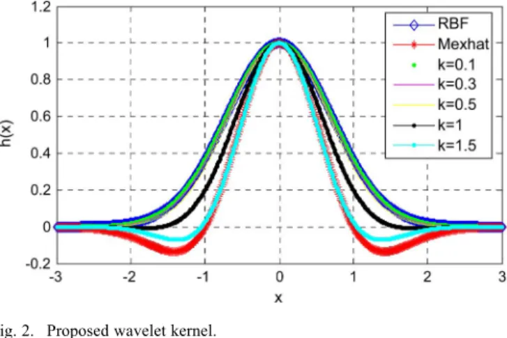
Based on the wavelet function in [27], a new wavelet mother function is proposed as follows:

(17) where is a parameter of the Gaussian kernel, and is a new parameter which controls the kernel shape. Fig. 2 shows the proposed kernel function when varies from 0 to 1.5

. When , is an RBF kernel; when , approximates the Mexhat kernel in the range of ; and when , is exactly the kernel proposed by Szu [27]. The proposed wavelet kernel is then obtained by substituting (17) into (15).

III. PROPOSEDWPP MODEL

The proposed WPP model consists of three components: preprocessing, WSVM-based wind speed prediction, and wind-speed-to-wind-power conversion, as shown in Fig. 3. The preprocessing includes data normalization and feature

(5)

Fig. 3. Structure of the proposed WPP model.

Fig. 4. Wind speed normalization.

representation. The WSVM plays a key role in the whole WPP model, on which the performance depends greatly. The output of the WSVM is wind speed, which is converted into wind power according to the power-wind-speed curves of the wind turbine generators (WTGs).

A. Data Normalization

The range of input data has influence on the performance of the SVM. Therefore, to avoid tuning the SVM parameters in (3) and (7) due to large variations of the input variables (i.e., wind speeds), the inputs are normalized by using the sigmoid function (18) where in this paper, is the nominal wind speed; and and and are the cut-in and cut-out wind speeds, respectively. There are two reasons for using the sigmoid function for data normalization. First, the sig-moid function can strictly map the original inputs, i.e., the real wind speeds, to the range of , as shown in Fig. 4, where the normalized values of 0.06 and 0.91 correspond to the original cut-in and cut-out wind speeds of 3.5 and 25 m/s, respectively. Second, the normalization using and makes the data trans-lation, rotation, and scaling invariant.

B. Feature Representation

Feature representation, which aims to extract certain charac-teristics from the original data, plays a key role in determining the performance of WPP. Improper features obtained from bad feature extraction will lead to poor regression in the WSVM. In

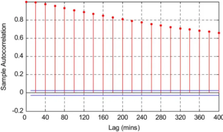
Fig. 5. Autocorrelations of input samples.

this paper, wind speed is selected as an intermediate variable, which is predicted by the proposed WSVM algorithm. The pre-dicted wind speed is then used to calculate the wind power ac-cording to the power-wind-speed characteristics of the WTGs. The reason for using wind speed as an intermediate variable in-stead of predicting wind power directly is that wind speed is a continuous variable while wind power discontinues at certain wind speeds (e.g., the cut-in, rated, and cut-out wind speeds). It is easier and more accurate to predict wind speed than wind power.

The WSVM input is expressed in the time series form as , where is called embed-ding dimension [23] and is determined from the autocorrelation coefficients of the data samples as follows:

(19) where and are the mean and standard deviation of the training data. Fig. 5 shows the autocorrelations of the original data. As shown in Fig. 5, the original data is highly linearly cor-related. Given a threshold of the autocorrelation coefficients, the embedding dimension can be determined. For example, if , then the former six samples are used as the input of the WSVM, i.e., .

C. Wind Speed-to-Wind Power Conversion

According to the predicted wind speed, the wind power is obtained from the wind turbines’ power-wind-speed character-istics. Fig. 6 shows the wind speed profile and the corresponding total power of 10 Vestas V-90 3-MW wind turbines at one grid point obtained from the NREL database, where the cut-in and cut-out wind speeds make the wind power curve discontinuous although the wind speed curve is continuous.

The wind-speed-to-wind-power conversion should take into account the wind turbine hysteresis effect [33]. This effect oc-curs during the period between the shutdown and restart of a wind turbine. The former event can be triggered when one of the cut-out criteria is met while the latter happens when the wind speed drops below a certain value. As shown in Fig. 6, the wind turbine is shut down at the 8th hour when the wind speed ex-ceeds 30 m/s and is not turned on until the wind speed drops

(6)

Fig. 6. Wind speed profile and corresponding wind power of 10 Vestas V-90 3-MW wind turbines obtained from the NREL database.

below 25 m/s. Once the wind speed is obtained, the following function is used to determine the wind power:

(20)

where is the predicted wind speed and is obtained from the wind-turbine-power-wind-speed curve (or power curve).

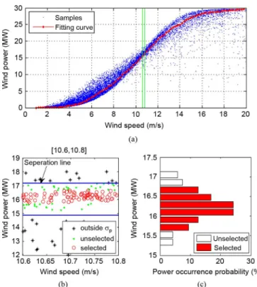
The function can be determined from the power curves provided by the wind turbine manufacturers. However, recent research has shown that there are advantages to determining an equivalent power curve (EPC) from the measured wind speed and power [34]. In this paper, the power curve is derived from the distribution of the Western data in 2004. Fig. 7 shows the process of generating the power curve. First, the wind speed data is allocated into multiple small intervals, where the length of each wind speed interval is 0.2 m/s, e.g., the interval m/s in Fig. 7(a). The mean and standard devia-tion of the corresponding wind powers are then calculated for the data in each wind speed interval. The wind speed sam-ples that the corresponding wind powers are located far away from the center, e.g., the samples (labeled as star) outside the range of in Fig. 7(b), are discarded.

Second, for each wind speed interval, after discarding the scattered data, the overall range of wind power is equally di-vided into 10 intervals. The power occurrence frequency (i.e., the number of samples in the th power interval) are cal-culated for each power interval, where . The nor-malized is taken as the power occurrence probability , i.e.,

. Fig. 7(c) shows the values of

in different intervals of wind power, which are approximately a normal distribution. The ten are then sorted in decreasing order. Given a threshold , thefirst intervals are selected according to the following criterion:

(21) Third, only the data in the selected power intervals are used. As shown in Fig. 7(c), the samples distributed between the

sepa-Fig. 7. Process of generating the power curve.

ration lines in Fig. 7(b) have high and low density values, re-spectively. Therefore, according to (21), the data with low den-sities in Fig. 7(c), which correspond to the data marked as dots in Fig. 7(b), are discarded, while the data marked as circles are selected. Finally, the wind power for the wind speed interval is calculated as

(22) where is the average wind power of the th power interval. Equation (22) is used to calculate the wind power for each wind speed interval. The power curve can then be obtained by sliding the wind power over all wind speed intervals, as shown in Fig. 7(a).

D. Evaluation

As in [9], the mean absolute error (MAE), mean absolute per-cent error (MAPE), and the standard deviation (Std) of MAE are used to measure the prediction performance. The definitions are expressed as

(23)

(24)

(25) where is the prediction horizon; is the nominal wind power; and are the step-ahead predicted and actual

(7)

wind power, respectively. Smaller values of MAE and Std imply the superior prediction performance of the model.

E. Parameter Selection

The three parameters, , , and , are determined by the fol-lowing procedure in order to implement the WSVM for WPP. First, choose andfix tofind the optimal . Then,fix to get the optimal ; and,finally, and arefixed to search exhaustively.

IV. MODELVALIDATION

The Western Dataset [35] created by 3TIER with oversight and assistance from NREL is used to validate the proposed WPP model. In the Western Dataset, NWP models were used to es-sentially recreate the historical weather for the western U.S. for the years of 2004, 2005, and 2006. The modeled data was sam-pled every 10 min temporally and every 2 km spatially. 3TIER modeled the power output of 10 wind turbines at 100 m above ground level on each grid point using a technique called the Sta-tistical Correction to Output from a Record Extension (SCORE) [36], which replicates the stochastic nature of the wind plant output. NREL modeled the hysteresis effect of the wind turbines to further replicate the real operation of wind plants. The data includes wind speed, rated power, SCORE-lite power, etc.

Sixty-eight grid points (i.e., 680 wind turbines of the same type) in a location 10 miles west of Denver, CO, were selected for simulation studies. Each data sample contains the average values of the wind speed and power among the 68 grid points at the same time. The time interval between the two nearest samples (called the time resolution) used as the inputs for the proposed WPP model is 20 min, where each new sample takes the average value of two consecutive samples in the original NREL dataset.

A. Prediction Schemes

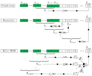
Since the prediction horizon is larger than the time resolu-tion of the data samples, different predicresolu-tion schemes can be used, including the fixed-step scheme, recursive scheme, and multi-WSVM scheme. Fig. 8 illustrates the principles of these schemes.

For a given prediction horizon , thefixed-step scheme pre-dicts the value at the next th step (e.g., hour) by using actual historical data only

(26) where is a nonlinear function representing the WSVM.

In the recursive scheme, the one-step scheme is applied itera-tively times to predict at the next th step. In each iteration, the predicted values from previous iterations are used as addi-tional historical data to predict at the next step

(27) The advantage of the recursive scheme is that it is accurate to predict the next-step value in each iteration. However, the prediction errors will accumulate over multiple steps, leading to larger errors at the th step compared to thefixed-step scheme.

Fig. 8. Principles of the three prediction schemes.

The multi-WSVM scheme predicts the value at the next th step by using multiplefixed-step predictions with different pre-diction horizons, e.g., , , and . Thefinal predicted value is obtained by the weighted sum of the values from all predictions

(28) where is the weight of the th prediction. Obviously the multi-WSVM prediction scheme becomes the fixed-step scheme if

and .

For a given prediction horizon, another important issue as-sociated with implementing the proposed WPP model is to de-termine the length of historical data (called the training length) used to train the WSVM. In order to determine the best training length, the WSVM is trained by using historical data with dif-ferent training lengths. The historical dataset (called the mod-eling dataset) contains the data before December 1, 2004, and is further divided into two parts: the training dataset and the vali-dation dataset. The training dataset contains 80% of the data in the modeling dataset while the validation dataset contains the re-maining 20% of the data. Fig. 9 shows the MAE and MAPE of the proposed WPP model as functions of training lengths from 30 days (November 1, 2004–November 30, 2004) to 110 days (August 23, 2004–November 30, 2004) for a prediction horizon of one hour using thefixed-step scheme. As shown in Fig. 9, it is not true that the longer the training length, the better the pre-diction performance. The MAE and MAPE decrease drastically with a training length of up to 70 days. However, after 70 days, the MAE and MAPE increase with the training length. There-fore, 70 days was selected as the best training length. Probably due to seasonal wind variations, the WSVM trained with too much historical data is too general to capture its intrinsic sea-sonal property.

Fig. 10 compares the MAE and Std of the three different schemes. The recursive scheme amplifies the errors step by

(8)

Fig. 9. Performance of the proposed WPP model versus training length for a prediction horizon of one hour using thefixed-step scheme.

Fig. 10. Comparison among the three prediction schemes.

step. Thefixed-step scheme is comparable to the multi-WSVM scheme but has an advantage over the multi-WSVM scheme in less computational cost. To predict hour-ahead wind speed, the multi-WSVM scheme needs to use multiple fixed-step predictions. Therefore, taking into consideration both compu-tational cost and accuracy, thefixed-step scheme is chosen to implement the WVSM for wind speed prediction. The training time with the fixed-step scheme is less than 5 min using a 2.8-GHz, 4-core, 8-GB RAM personal computer when the training length is set at 70 days.

B. WPP Using the WSVM

The proposed WSVM-based model with the fixed-step scheme is applied for WPP with different prediction horizons. The testing dataset contains the data from December 1, 2004 to December 7, 2004 of the Western Dataset while the training dataset contains the data of 70 days before December 1, 2004, i.e., the training length is chosen to be 70 days. The parameters of the WSVM are determined by the method in Section III-E based on the performance of one hour (1 h)-ahead WPP. The

final values of the parameters are listed in Table I.

The 1-, 2-, and 3-h-ahead WPP results using the proposed WSVM-based model with thefixed-step scheme are shown in

TABLE I PARAMETERS OF THEWSVM

Fig. 11. One-hour-ahead WPP using the WSVM model andfixed-step scheme.

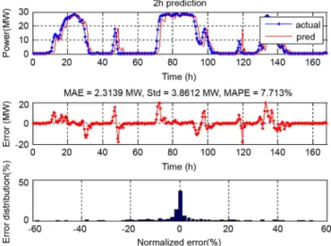
Fig. 12. Two-hours-ahead WPP using the WSVM model and fixed-step scheme.

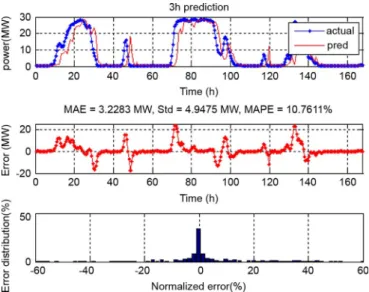
Figs. 11–13, respectively, where the normalized error is defined as: . In all cases, the predicted wind power follows the actual wind power closely. The normalized errors of most samples fall between 10% and 10%. More than 70% of the normalized errors are less than 5% in the case of 1-h-ahead WPP. Approximately 60% and 50% normalized errors are less than 5% in 2- and 3-h-ahead predictions, respectively. A large error occurs when the wind speed changes drastically. More-over, from the perspective of statistics, the larger the prediction horizon, the more uncorrelated data used which leads to a larger prediction error. Therefore, the performance of the proposed model degrades with the increase of the prediction horizon.

In order to show the effectiveness of the model, 1 to 30 days of consecutive data (December 1, 2004–December 30, 2004) were

(9)

Fig. 13. Three-hours-ahead WPP using the WSVM model and fixed-step scheme.

Fig. 14. MAPE as a function of the testing length.

tested using thefixed-step scheme. Fig. 14 shows the MAPE as a function of the testing length for 1- and 2-h prediction hori-zons. The MAPE is almost constant during thefirst 10 days and increases when the testing length further increases. However, it is reasonable to say that the proposed WAVM model offers acceptable WPP performance for 30 days without the need of retraining the model. Beyond 10 or 30 days, the model can be retrained to ensure that the prediction performance is accept-able, while retraining the model only takes a few minutes.

C. Comparison of Three WPP Models

The proposed WSVM-based model is compared with the persistence and RBF-SVM models to further evaluate its performance. The persistence model is a classical benchmark model in which the predicted values at any future time within the prediction horizon are set at the current value. The results are shown in Figs. 15 and 16, where the testing dataset contains the data from December 1, 2004 to December 7, 2004 of the Western Dataset. As shown in Fig. 15, both SVM-based models significantly outperform the persistence model in terms of prediction accuracy. Furthermore, the WSVM model is always better than the RBF-SVM model. Fig. 16 compares the actual

Fig. 15. Comparison among the persistence, RBF-SVM, and WSVM models.

Fig. 16. Comparison between the RBF-SVM and WSVM models.

wind power with the predicted wind power from the WSVM model and RBF-SVM model. The predicted value using the WSVM model follows more closely the observation than that using the RBF-SVM model. The possible reason is that the proposed kernel is better than the RBF kernel.

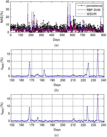
To further testify the superiority of the proposed model over the persistence and RBF-SVM models, the three models were applied to predict wind power for 900 days (April 11, 2004–Oc-tober 8, 2006). The WSVM and RBF-SVM models were up-dated every 10 days. Fig. 17(a) compares the daily mean values of the normalized absolute error (NAE) of the three models for a prediction horizon of one hour, where the NAE is defined as . As shown in Fig. 17(a), the WSVM and RBF-SVM models achieve lower NAEs than the persistence model. To clearly show that the WSVM is better than the RBF-SVM, the NAE difference,

, of the two models was calcu-lated. Fig. 17(b) and (c) show the values of for 1- and 2-h-ahead predictions, respectively. The mean value of over 900 days is 0.5% for both the 1-h-ahead and the 2-h-ahead predictions. The NAEs of the WSVM are a little smaller than those of the RBF-SVM during most times. However, at certain times when the wind speed changes drastically, which is more difficult to predict, the WSVM can predict the wind power much more accurately than the RBF-SVM.

(10)

Fig. 17. Comparison of the three models for 900 days. (a) NAEs of the three models. (b) for 1-h-ahead prediction. (c) for 2-h-ahead prediction.

V. CONCLUSION ANDDISCUSSION

This paper has proposed a WSVM-based model, which com-bines wavelet analysis and SVM, for short-term WPP. A new SVM kernel has been proposed based on a multidimensional wavelet function that can approximate arbitrary functions. The new kernel can vary among different kernels according to spe-cific applications, which makes the WSVM acquire better gen-eralization ability than the SVM with an RBF kernel. More-over, the proposed model utilizes the principle of wavelet anal-ysis to facilitate nonlinear characteristic extraction of the wind data for WPP. Therefore, it is not surprising that the proposed WSVM-based model is superior to the RBF-SVM-based model. Simulation studies have been carried out for a dataset obtained from the NREL. Results have shown that the WSVM model is effective for short-term WPP, significantly outperforms the per-sistence model, and is better than the RBF-SVM model in terms of prediction accuracy.

However, the history data becomes less correlated with the in-crease of the prediction horizon. Therefore, the proposed model gradually failed to catch up to the trend of wind variations. The proposed model is suitable for short-term WPP. For longer-term WPP, extra meteorological variables, such as temperature and pressure, should be used and combined with the NWP to im-prove the prediction accuracy.

REFERENCES

[1] U.S. Department of Energy, 20% wind energy by 2030: In-creasing wind energy’s contribution to U.S. electricity supply DOE/GO-102008-2567, Jul. 2008 [Online]. Available: http://www. nrel.gov/docs/fy08osti/41869.pdf

[2] Global Wind Energy Council, Global wind energy outlook 2008 Oct. 2008 [Online]. Available: http://www.gwec.net/index.php?id=92 [3] European Wind Energy Association, Focus on 2030: EWEA Aims for

22% of Europe’s Electricity by 2030, Wind Directions Nov./Dec. 2006 [Online]. Available: http://www.ewea.org/fileadmin/ewea_documents/ documents/publications/WD/2006_november/WD26-focus.pdf [4] P. Chen, P. Siano, B. Bak-Jensen, and Z. Chen, “Stochastic optimization

of wind turbine power factor using stochastic model of wind power,”

IEEE Trans. Sustain. Energy, vol. 1, no. 1, pp. 19–29, Apr. 2010. [5] J. Liang, W. Qiao, and R. G. Harley, “Feed-forward transient current

control for low-voltage ride-through enhancement of dfig wind tur-bines,”IEEE Trans. Energy Convers., vol. 25, no. 3, pp. 836–843, Sep. 2010.

[6] J. Kabouris and F. D. Kanellos, “Impacts of large-scale wind pene-tration on designing and operation of electric power systems,”IEEE Trans. Sustain. Energy, vol. 1, no. 2, pp. 107–114, Jul. 2010. [7] V. Galdi, A. Piccolo, and P. Siano, “Designing an adaptive fuzzy

controller for maximum wind energy extraction,”IEEE Trans. Energy Convers., vol. 23, no. 2, pp. 559–569, Jun. 2008.

[8] C. Monterio, R. Bessa, and V. Miranda, Wind Power Forecasting: State-of-the-Art 2009 Argonne National Laboratory, ANL/DIS-10-1, Nov. 2009 [Online]. Available: http://www.dis.anl.gov/pubs/65613.pdf [9] H. Y. Zheng and A. Kusiak, “Prediction of wind farm power ramp rates: A data-mining approach,”ASME J. Solar Energy Eng., vol. 131, pp. 031011-1–031011-8, Aug. 2009.

[10] L. Landberg and S. J. Watson, “Short-term prediction of local wind conditions,”J. Wind Eng. Ind. Aerodynamics, vol. 89, pp. 235–245, 2001.

[11] N. G. Mortensen, D. N. Heathfield, L. Landberg, O. Rathmann, I. Troen, and E. L. Petersen, Wind Atlas Analysis and Application Pro-gram: WAsP 8.0 Help Facility. Roskilde: Risø National Laboratory, 2003.

[12] L. Landberg, G. Giebel, H. A. Nielsen, T. Nielsen, and H. Madsen, “Short-term prediction-an overview,” Wind Energy, vol. 6, pp. 273–280, 2003.

[13] T. G. Barbounis, J. B. Theocharis, M. C. Alexiadis, and P. S. Dokopoulos, “Long-term wind speed and power forecasting using local recurrent neural network models,”IEEE Trans. Energy Convers., vol. 21, no. 1, pp. 273–284, Mar. 2006.

[14] H. Madsen, H. A. Nielsen, and T. S. Nielsen, “A tool for predicting the wind power production of off-shore wind plants,” inProc. Copen-hagen Offshore Wind Conf. Exhibition, Danish Wind Industry Assoc., Copenhagen, Denmark, Oct. 2005.

[15] T. Nielsen, H. A. Madsen, and J. Tøfting, “Experiences with statistical methods for wind power prediction,” inProc. Eur. Wind Energy Conf., Nice, 1999, pp. 1066–1069.

[16] G. Sideratos and N. D. Hatziargyriou, “An advanced statistical method for wind power forecasting,”IEEE Trans. Power Syst., vol. 22, no. 1, pp. 258–265, Feb. 2007.

[17] G. Giebel, L. Landberg, T. Nielsen, and H. Madsen, “The zephyr project-the next generation prediction system,” inProc. Global Wind Power Conf., Paris, France, Apr. 2002.

[18] S. Rajagopalan and S. Santoso, “Wind power forecasting and error analysis using the autoregressive moving average modeling,” inProc. IEEE Power & Energy Society General Meeting 2009, Calgary, Al-berta, Canada, Jul. 26–30, 2009.

[19] G. N. Kariniotakis, G. S. Stavrakakis, and E. F. Nogaret, “Wind power forecasting using advanced neural networks models,”IEEE Trans. En-ergy Convers., vol. 11, no. 4, pp. 762–767, Dec. 1996.

[20] J. P. S. Catalao and V. M. F. Mendes, “An artificial neural network approach for short-term wind power forecasting in portugal,” inProc. 15th Int. Conf. Intelligent System Applications to Power System, Mar. 1, 2009, vol. 17.

[21] M. A. Mohandes, S. Rehman, and T. O. Halawani, “A neural net-works approach for wind speed prediction,”Renew. Energy, vol. 13, pp. 345–354, Mar. 1998.

[22] K. R. Miller and V. Vapnik, Using Support Vector Machine for Time Series Prediction. Cambridge, MA: MIT Press, 1999, pp. 243–253.

(11)

[23] K. Speelakshmi and P. R. Kumar, “Performance evaluation of short term wind speed prediction techniques,”Int. J. Comput. Sci. Netw. Se-curity, vol. 8, no. 8, pp. 162–169, Aug. 2008.

[24] L. Cao and R. Li, “Short-term wind speed forecasting model for wind farm based on wavelet decomposition,” inProc. Third Int. Conf. Elec-tric Utility Deregulation and Restructuring and Power Technologies, Nanjing, China, Apr. 2008, pp. 2525–2529.

[25] R. R. B. De Aquino, M. M. S Lira, J. B. De oliverira, M. A. Carvalho, O. N. Neto, and G. J. De almeida, “Application of wavelet and neural network models for wind speed and power generation forecasting in a brazilian experimental wind park,” inProc. Int. Joint Conf. Neural Networks, Atlanta, GA, Jun. 14–19, 2009, pp. 172–178.

[26] A. Silva, L. Moulin, and A. J. R. Reis, “Feature extraction via multires-olution analysis for short-term load forecasting,”IEEE Trans. Power Syst., vol. 20, no. 1, pp. 189–198, Feb. 2005.

[27] H. H. Szu, B. A. Telfer, and S. Kadambe, “Neural network adaptive wavelets for signal representational and classification,”Opt. Eng., vol. 31, pp. 1907–1916, Nov. 1992.

[28] A. Smola and B. Schölkopf, “A tutorial on support vector regression,”

Statist. Comput., vol. 14, no. 2, pp. 199–222, Sep. 2003.

[29] V. Vapnik, The Nature of Statistical Learning Theory. New York: Springer, 1995.

[30] Q. H. Zhang and A. Benveniste, “Wavelet networks,”IEEE Trans. Neural Netw., vol. 3, no. 6, pp. 889–898, Nov. 1992.

[31] I. Daubechies, “The wavelet transform, time-frequency localization and signal analysis,” IEEE Trans. Inf. Theory, vol. 36, no. 5, pp. 961–1005, Sep. 1990.

[32] L. Zhang, W. Zhou, and L. Jiao, “Wavelet support vector machine,”

IEEE Trans. Syst., Man, Cybern., vol. 34, no. 1, pp. 34–39, Feb. 2004. [33] L. Horvath, “The influence of high wind hysteresis effect on wind tur-bine power production as bura-dominated site,” inProc. Eur. Wind En-ergy Conf. Exhibition, Milan, Italy, May 2007.

[34] G. Giebel, L. Landberg, G. Kariniotakis, and R. Brownsword, “State-of-the-art on methods and software tools for short-term pre-diction of wind energy production,” inProc. Eur. Wind Energy Conf. Exhibition, Madrid, Span, 2003.

[35] C. W. Potter, D. Lew, J. McCaa, S. Cheng, S. Eichelberger, and E. Grimit, “Creating the dataset for the western wind and solar integra-tion study (U.S.A),” inProc. 7th Int. Workshop on Large Scale Integra-tion of Wind Power and on Transmission Networks for Offshore Wind Farms, Madrid, Spain, May 26–27, 2008.

[36] C. W. Potter, H. A. Gil, and J. McCaa, “Wind power data for grid inte-gration studies,” inProc. 2007 IEEE Power Engineering Society Gen-eral Meeting, Tampa, FL, Jun. 2007.

Jianwu Zeng(S’10) received the B.Eng. degree in electrical engineering from Xi’an University of Tech-nology, Xi’an, China, in 2004, and the M.S. degree in control science and engineering from Zhejiang Uni-versity, Hangzhou, China, in 2006. Currently, he is working toward the Ph.D. degree at the University of Nebraska-Lincoln, Lincoln, NE.

In 2006, he joined Santak Electronic (Shenzhen) Co., Ltd., Shenzhen, China, where he was an Elec-tronic Engineer. He was involved in research and de-velopment of soft switching and DC–DC converters. His research interests include power electronics and renewable energy.

Wei Qiao (S’05–M’08) received the B.Eng. and M.Eng. degrees in electrical engineering from Zhejiang University, Hangzhou, China, in 1997 and 2002, respectively, the M.S. degree in high performance computation for engineered systems from Singapore-MIT Alliance (SMA), Singapore, in 2003, and the Ph.D. degree in electrical engineering from Georgia Institute of Technology, Atlanta, GA, in 2008.

From 1997 to 1999, he was an Electrical Engineer with China Petroleum and Chemical Corporation (Sinopec). Currently, he is the Harold and Esther Edgerton Assistant Professor with the Department of Electrical Engineering at the University of Ne-braska-Lincoln (UNL), Lincoln, NE. His research interests include renewable energy systems, smart grids, microgrids, power system control and optimiza-tion, condition monitoring and fault diagnosis, energy storage systems, power electronics, electric machines and drives, and high-performance computation for electric power and energy systems. He is the author or coauthor of three book chapters and more than 90 papers in refereed journals and international conference proceedings.

Dr. Qiao is an Associate Editor of the IEEE TRANSACTIONS ONINDUSTRY APPLICATIONS, the Chair of the Sustainable Energy Sources Technical Thrust of the IEEE Power Electronics Society, and the Chair of the Task Force on Intelli-gent Control for Wind Plants of the IEEE Power and Energy Society. He is the Technical Program Cochair of the 2012 IEEE Symposium on Power Electronics and Machines in Wind Applications (PEMWA 2012) and was the Technical Pro-gram Cochair and Finance Cochair of PEMWA 2009. He was the recipient of a 2010 National Science Foundation CAREER Award, the 2010 IEEE Industry Applications Society Andrew W. Smith Outstanding Young Member Award, the 2011 UNL Harold and Esther Edgerton Junior Faculty Award, and the 2011 UNL College of Engineering Edgerton Innovation Award.