Modelling rainfall-runoff processes in lowland catchments

(1)

(2)

Promotor

Prof.Dr R. Uijlenhoet

Professor of Hydrology and Quantitative Water Management Wageningen University

Co-promotor Dr A.J. Teuling

Assistant professor, Hydrology and Quantitative Water Management Group Wageningen University

Other members

Prof.Dr A.A.M. Holtslag, Wageningen University

Prof.Dr N.C. van de Giesen, Delft University of Technology

Dr L. Pfister, Centre de Recherche Public Gabriel Lippmann, Luxembourg Prof.Dr T. Wagener, University of Bristol, United Kingdom

(3)

Modelling

rainfall-runoﬀ processes

in lowland catchments

Claudia Brauer

Thesis

submitted in fulfilment of the requirements for the degree of doctor at Wageningen University

by the authority of the Rector Magnificus Prof.Dr M.J. Kropﬀ

in the presence of the

Thesis Committee appointed by the Academic Board to be defended in public

on Friday 11 April 2014 at 1.30 p.m. in the Aula.

(4)

Modelling rainfall-runoﬀ processes in lowland catchments vi + 98 pages

PhD thesis, Wageningen University, Wageningen, The Netherlands (2014) With references, with summaries in English and Dutch

(5)

1 |

Introduction

A

round the world, lowland areas are often densely populated and centers of economic activityand transportation. The lack of topography, however, makes them vulnerable to flooding, climate change, and deterioration of water quality. Hydrological models can be used by water managers as a tool for early warning, risk assessment and infrastructure design. However, the models that are commonly used in lowland areas are often high-dimensional (groundwater or hydraulic) models. Low-dimensional models have typically been designed for use in mountainous catchments. The title of this thesis reflects the two-part research question: (1) what are the dominant catchment processes determining a lowland river’s response to rainfall and (2) how can these processes be represented in simple hydrological models? For both of these questions, I focussed on topics which are important for lowland areas: (1) the relation between catchment storage and discharge, (2) the coupling between shallow groundwater and unsaturated zone, (3) activation of flowroutes at diﬀerent stages of wetness and (4) the feedback between groundwater and surface water.

1.1 Context and motivation

1.1.1 Lowlands around the world

Lowlands can be found all over the world, in differ-ent climates, geological settings and even altitudes. A universally accepted definition of lowlands does not exist, because people from different parts of the world have different views of this type of landscape. People from mountainous areas may call the lower river reaches at several hundreds of meters altitude lowlands (e.g. Kao et al., 2012, who classify areas below 1000 m as lowland in Taiwan). The Dutch, on the other hand, call the part of their country above sea level the “High Netherlands” (Witte et al., 2012). In this thesis, lowlands are defined as areas in which hydrological processes are influenced by shallow groundwater. This means that according to this definition, lowlands can also occur well above sea level and that low-lying arid areas are not con-sidered in this thesis.

Shallow (phreatic) groundwater tables occur all over the world (often in river deltas): 16 % of world’s land surface has groundwater tables shallower than 2 m, and 22 % shallower than 4 m (Fig. 1.1; data from Fan et al., 2013). Many of these areas have been reclaimed from sea or marshes by drainage and control of groundwater levels (and sometimes surface water levels). Reclaimed land can be found in coastal areas and river floodplains across diﬀer-ent climate zones, from coastal wetlands in Indone-sia and the Nile delta in Egypt to the Great Lakes in North-America (see Wandee, 2013, for an overview). This indicates that being able to understand and model lowland-specific hydrologic processes is ben-eficial for scientists and practitioners around the world.

Lowland catchments can be divided into freely draining ones and controlled ones, The latter are of-ten called polders (Wandee, 2013).Freely draining lowland catchments have slightly sloping land

sur-faces and gravitational forces cause water to flow downhill naturally. Polders are flat and because their land surfaces are below their surroundings, water has to be removed by pumping. In reality, the distinction between the two types is less clear. In many freely draining areas, groundwater and sur-face water levels are controlled through the instal-lation of drainpipes, ditches and weirs. In polder areas, water follows local (micro)topographical gra-dients to the surface water network.

1.1.2 Challenges in lowland areas

Lowlands areas, especially those in river deltas, are often densely populated and centers of agricultural production, economic activity and transportation. Therefore, socio-economic consequences of natural hazards are especially large in these areas (Day et al., 2007). In addition, the lack of topography in-creases their vulnerability to diﬀerent threats:

1. Floods are a major hazard in lowland areas. Lowlands are often located in river deltas and are threatened simultaneously by high sea lev-els (coastal floods), high river discharges (flu-vial floods) and large precipitation events (plu-vial floods) (e.g. Zhang et al., 2008; Hidayat, 2013). Lowlands are not only more prone to flooding, but flood damage is also large due to the high density of population, infrastructure and economic activity (Jonkman et al., 2008). Flood risk, loosely defined as the product of probability and damage (e.g. Merz et al., 2004), is therefore extra large.

2. Climate change has a double eﬀect on low-land catchments (Vellinga et al., 2009; Kwadijk et al., 2010). Firstly, temperature rise causes sea level rise, reducing drainage gradients in coastal lowlands (Bormann et al., 2012). Some areas will not be able to discharge water natu-rally anymore and surface water will have to be pumped out, or the land will be reclaimed by the

(8)

Groundwater depth [m] 0−2 2−4 >4

Figure 1.1: Lowland areas around the world: locations with shallow groundwater (based on data from Fan et al., 2013).

sea (Nicholls et al., 1999). In addition, upward (brackish) seepage will increase, leading to a decrease in agricultural production and food security (Oude Essink, 2001; Wassmann et al., 2004; Witte et al., 2012). More fresh water will have to be supplied upstream to flush the surface water network and reduce salt concen-trations. Secondly, heavy precipitation events have become more frequent and intense in the past century in Europe and North America. This trend will very likely continue in the current century (Field et al., 2012; IPCC, 2013), leading to increased (flash) flood risk. The simultaneous occurrence of high river discharges and high sea levels poses an increased threat as rivers are unable to discharge to the sea (Kew et al., 2011).

3. Land use changeis common in densely popu-lated lowland areas (Bouwer et al., 2010). Ru-ral areas are transformed into urban areas with more paved surfaces and less water storage capacity. In wetlands, a large fraction of the area is covered by surface water, which at-tenuates heavy precipitation events (Thompson et al., 2009). When wetlands are drained, peak discharges will increase (Azous and Horner, 2010). To increase food production, agricultural fields around the world are controlled more in-tensely to optimize groundwater levels and re-duce crop yield loss caused by waterlogging and drought. This results in fields with more drain-pipes, channels, weirs, surface water supply installations and pumps (Elfert and Bormann,

2010).

4. Water qualitydeterioration is common in low-land areas because intensive agriculture causes a large influx of nutrients into the surface wa-ter (Lam et al., 2012; Neal et al., 2012). In ad-dition, algal blooms may occur due to low flow velocities caused by the small topographic gra-dients. Legislation, such as the European Water Framework Directive, has been implemented to improve the ecological and chemical status of water systems (Howden et al., 2009). Nu-merous research projects have been carried out over the past decades to understand nutrient dynamics and the relation between nitrate and phosphate concentrations and flowpaths in in-tensively drained and managed lowland areas (e.g. Van den Eertwegh, 2002; Rozemeijer et al., 2010a; Van der Velde, 2011; Delsman et al., 2013).

5. Land subsidence is more common and more problematic in coastal lowland areas (Ericson et al., 2006). Peat is formed in waterlogged de-pressions in the landscape, but when old peat soils are drained for agricultural use, peat can oxidize and soils subside (Wösten et al., 1997). The threat of subsidence forces water man-agers to control groundwater levels to mini-mize oxidation (Gambolati et al., 2003). Low freely draining catchments may sink below the drainage base (the sea), and pumping may be required to remove excess water.

(9)

cen-1.2. Hydrological models | 3

tury (Montanari et al., 2013). Because lowland areas are densely populated, many water man-agers, governmental agencies, (re-)insurance companies and the general public benefit from accurate predictions of floods and droughts (Borga et al., 2011; Demeritt et al., 2013). In many countries, water managers have a legal obligation to investigate the hydrological eﬀect of change in management, land use and climate in depth to reduce uncertainty about the future. The general public is increasingly aware of their surroundings, is more used to having access to data and predictions and is less willing to ac-cept damage caused by natural hazards (Mess-ner and Meyer, 2006).

To mitigate natural and human disasters, hydrologi-cal models can be used by water managers as a tool for risk assessment and infrastructure design.

1.2 Hydrological models

Many types of hydrological models exist, with diﬀer-ent degrees of complexity. The appropriate degree of complexity depends on the objectives of the model study and the catchment the model is applied to (Wa-gener et al., 2001). Black boxmodels are typically the least complex model type. They have hardly any physical background: relations between vari-ables (often rainfall and discharge) are determined empirically, without predefining a model structure based on process understanding. Examples of black box models are the unit hydrograph (Clark, 1945) and artificial neural networks (Bishop, 1995; Reed and Marks, 1998). The most complex model type is usually described with the termphysically-based, although this name is controversial because other model types are also based on physics (see e.g. Beven and Young, 2013). These models contain de-tailed, spatially distributed descriptions of measur-able catchment properties (e.g. soil type, eleva-tion, vegetaeleva-tion, channel dimensions). They are typ-ically based on (partial) diﬀerential equations (e.g. Richards’ equation for the unsaturated zone or the St. Venant equation for open water). Examples of this model type are SHE (Abbott et al., 1986) and MIKE-SHE (Refsgaard and Storm, 1995).

Between detailed, spatially distributed models and black box models lies the class of parametric rainfall-runoﬀ models. This type of model simpli-fies hydrological systems into a collection of reser-voirs and flowroutes, capturing the essence of the relevant hydrological processes, while restricting the number of parameters (Wagener and Wheater, 2004). Parametric models are spatially lumped: variables and parameters are eﬀective catchment values (not necessarily the catchment average).

Widely used examples of parametric rainfall-runoﬀ models are the Tank Model (Sugawara et al., 1974), PDM (Moore, 1985), HBV (Bergström and Fors-man, 1973), the Sacramento Model (Burnash, 1995), ARNO (Todini, 1996), SWAT (Arnold et al., 1998) and GR4J (Edijatno et al., 1999; Perrin et al., 2003). However, these models have all been developed for mountainous catchments and errors may arise when applied to lowland catchments, because processes (e.g. capillary rise) are not accounted for and condi-tions (e.g. no influence of surface water on ground-water) are not met. Examples of the resulting prob-lems are presented by Bormann and Elfert (2010), who used WaSiM-ETH (Schulla and Jasper, 2007) and Koch et al. (2013), who used SWAT, both in north-eastern Germany.

Water managers in lowland areas often use com-plex hydrological models. MIKE-SHE (Refsgaard and Storm, 1995), HEC-RAS (Brunner, 1995) and SOBEK (Deltares, 2013) have detailed schematisa-tions of surface water networks to simulate the com-plex flow routing in intensively drained areas. HY-DRUS (Simůnek et al., 2008) and SWAP (Van Dam et al., 2008) have detailed vertical schematisations to simulate unsaturated-saturated zone coupling. Regional groundwater models, such as MODFLOW (McDonald and Harbaugh, 1984), account for seep-age and lateral groundwater flow. Combinations of several of these models can be used to account for groundwater-surface water feedbacks, such as SHE (Abbott et al., 1986), HydroGeoSphere (Therrien et al., 2006) SIMGRO (Querner, 1988; Van Walsum and Veldhuizen, 2011) or NHI (Prinsen and Becker, 2011). However, complex models have important disadvantages and simple models important advan-tages:

1. Overparameterisation – Model parameters ac-count for diﬀerences in response times or reces-sion shapes between catchments with the same dominant processes (represented by the model structure). With too many parameters, an inap-propriate model structure can be compensated for by mathematically fitting the model to the calibration data (Kirchner, 2006). An overpa-rameterised model may perform well during cal-ibration, but unsatisfactorily during validation (Perrin et al., 2001) and in diﬀerent (future) cli-mate regimes (e.g. Seibert, 1999a).

2. Parameter identification – The risk of parame-ter dependence and equifinality (where diﬀer-ent combinations of parameter values to lead to similar results, Beven and Binley, 1992; Uhlen-brook et al., 1999) increases with the number of parameters. With one objective function, typi-cally only 3 to 5 parameters can be identified (Jakeman and Hornberger, 1993; Beven, 1989). Multi-objective calibration allows more

(10)

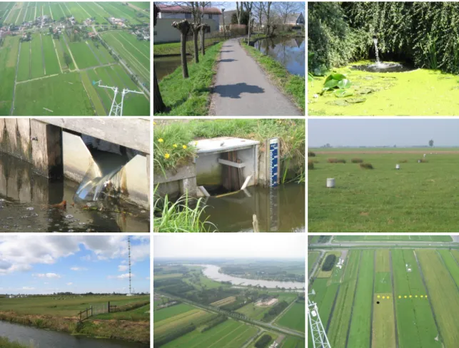
param-Figure 1.2: Discharge mechanisms at diﬀerent scales in the Cabauw polder. Top row: animal burrow, soil cracks, gully, drainpipe. Bottom row: local ponding, field-scale ponding, surface water network.

eters to be calibrated (e.g. Gupta et al., 1998; Efstratiadis and Koutsoyiannis, 2010), but for many catchments only discharge data are avail-able (Soulsby et al., 2008). It is therefore bene-ficial when the eﬀect of each parameter on the discharge time series can be identified. 3. Physical representation – A simple,

paramet-ric model structure enables users to quickly grasp the process covered by each model ele-ment and the influence of each parameter. Val-ues of eﬀective model parameters cannot be de-termined with point measurements (Wagener, 2003; Vrugt et al., 2005), but model param-eters do have physical connotations and can be explained qualitatively from catchment char-acteristics and field experience (Seibert and McDonnell, 2002). The eﬀect of small-scale heterogeneity on catchment-scale processes is included implicitly in the model parameters (Beven, 1995; Kirchner, 2006; McDonnell et al., 2007).

4. Practical applicability – Computational eﬃ-ciency facilitates operational forecasting and data assimilation (Liu et al., 2012; Rakovec et al., 2012). Ensembles can be generated for diﬀerent forcing data or parameter sets to in-dicate predictive uncertainty (Krzysztofowicz, 2001). In addition, more complex and time-consuming algorithms can be used for

calibra-tion (e.g. DREAM by Vrugt et al., 2008) or pa-rameter uncertainty estimation (e.g. GLUE by Beven and Binley, 1992). Avoiding the need to specify channel cross-sections and soil layers for each catchment can also be advantageous.

1.3 Characteristics of lowland

catchments

In this section we discuss some characteristics which aﬀect hydrological processes in lowland catchments and how they are represented in some widely used rainfall-runoﬀ models.

1.3.1 Groundwater-unsaturated zone coupling

Whereas in most models percolation is assumed to be driven by downward gravitational forces only, the vertical profile of moisture content in lowland soils is influenced by capillary forces associated with the presence of a shallow groundwater table. Percola-tion is slower and evapotranspiraPercola-tion remains high in dry periods, because storage deficits are replen-ished by capillary rise (e.g. Hopmans and van Im-merzeel, 1988; Stenitzer et al., 2007). Therefore, the vadose zone and the groundwater zone form a tightly coupled system and feedbacks should be

(11)

in-1.3. Characteristics of lowland catchments | 5

cluded in models for lowland catchments (Chen and Hu, 2004). In addition, when groundwater rises to the soil surface, the unsaturated zone shrinks and its storage capacity decreases. It is therefore important to include a dynamic unsaturated zone in the model, which is influenced by the surface fluxes precipita-tion and evapotranspiraprecipita-tion as well as by the (dy-namic) groundwater table below.

Many conceptual rainfall-runoﬀ models, e.g. HBV, the Sacramento model and the Wageningen Model, contain separate reservoirs for soil mois-ture and groundwater, allowing only downward movement of groundwater without considering feed-backs. One version of PDM does reduce recharge when the soil ceases to be freely draining (Moore, 2007). Catchments can also be simplified to a sin-gle nonlinear reservoir, without discriminating be-tween the saturated and unsaturated zone (Kirchner, 2009), which will be shown to yield limited success in the lowland Hupsel Brook catchment (Chapter 4). Quasi-steady state approaches have also been devel-oped for implementation in distributed models e.g. by Koster et al. (2000), Bogaart et al. (2008) and Van Walsum and Groenendijk (2008).

1.3.2 Shallow groundwater and plant water stress

Vegetation in lowland catchments is hardly affected by water stress, which is one of the drivers for agri-cultural production. Water is not only made avail-able through physical processes (capillary rise), but also through physiological ones: when plants have exhausted the readily available moisture in the top soil, deeper roots are used (Zencich et al., 2002), and vertical roots grow deeper (Canadell et al., 1996; Weir and Barraclough, 1986; Teuling et al., 2006) and more quickly (Zeng et al., 2013). Because plants adapt to spatial variability in moisture content, wa-ter uptake and its vertical distribution depend pri-marily on the availability of moisture in the whole root zone (Jarvis, 1989). As roots in lowlands often extend to close to the groundwater table, plants can adapt fully to dry periods and evapotranspiration re-duction hardly occurs (Schenk and Jackson, 2002). This dynamic system of different plant species with varying stages of root development and spatially and temporally varying groundwater depths is complex, but not all complexity may be necessary to include in a model for runoff simulations (Van der Ploeg et al., 2012).

In some rainfall-runoﬀ models for areas with deep water tables, a separate root zone is included, e.g. in SWAT and TOPMODEL, which exhibits a dif-ferent behaviour than the unsaturated zone below. We assume that in lowlands, this distinction cannot be made because the whole unsaturated zone can be

Q [mm h − 1] 0 0.5 ₁₀ 0 P [mm h − 1] a dG [m] 1.2 0.8 b C [mg l − 1 ] ● ●● ●● ● ●_{●●●●●}●●● ●●●●● ● ●●●●● ● ●●●●_{●●●●●●} ●●● ● ● ●●●●●●●● ● ●●● ● ● ●●● ● ● ● ● ●●● ● ●●●●● ● ●● ● ● ● ● ● ● ● 0 0.4 0.8 c Phosphorus C [mg l − 1 ] ● ● ● ● ●●●● ●●●● ●● ● ● ● ●●●●●● ●● ● ● ● ●● ● ● ● ● ● ●● ● ●● ● ●● ●●●●●●●●● ● ● ● ● ● ● ●● ●● ●● ● ● ● ●● ●●●● ●● ● ● ● ● ● ●● 20 40 d Nitrate C [mg l − 1 ] ● ●● ●●● ●●●●●●●●● ●●●● ● ● ●●●●● ● ●●●●●●● ●●● ●●● ●●●●●● ●●●●●●●● ● ● ●●●●● ● ●● ●●●●●● ●●● ●●● ●●● ● ● ● 30 50 e Chloride

10 Sep 1 Oct 20 Oct 1993

Figure 1.3: Activation of diﬀerent flow paths re-vealed by water quality data measured at the out-let of the Hupsel Brook catchment.(a)Precipitation and discharge.(b)Groundwater depth at the meteo-rological station. (c)Phosphorus concentration (in-dicator for overland flow, Rozemeijer et al., 2010b), (d) Nitrate concentration (indicator for drainpipe flow, Van der Velde et al., 2010b). (e)Chloride con-centration (indicator for groundwater flow, Van der Velde et al., 2010a).

used by plant roots. The variation of plant species within a catchment is sometimes represented by running a model for diﬀerent vegetation types sepa-rately and multiplying the resulting discharge out-put with the fraction of that vegetation type (Van Dam et al., 2008).

1.3.3 Wetness-dependent flowroutes When the soil wetness increases, different flowpaths are activated: from groundwater flow (Hall, 1968), to natural macropores (Mosley, 1979; Beven and Germann, 1982; McDonnell, 2003; Beven and Ger-mann, 2013) and drainpipes (Tiemeyer et al., 2007; Rozemeijer et al., 2010a; Van der Velde et al., 2010b) and eventually to surface runoff (Dunne and Black, 1970; Brauer et al., 2011; Appels et al., 2011). Fig-ure 1.2 provides examples of discharge mechanisms in lowland catchments at different scales.

Stream water chemistry is increasingly being used to detect hydrological flow paths (e.g. Soulsby et al., 2004; Tetzlaff et al., 2007; Delsman et al., 2013). Records of phosphorus, nitrate and chloride concentrations measured at the outlet of the Dutch Hupsel Brook catchment confirm the activation of different flow routes at different stages of catchment

(12)

Figure 1.4: Schematic representation of the topics of this thesis: (1) storage-discharge relations, (2) groundwater-unsaturated zone coupling, (3) wetness-dependent flowroutes and (4) groundwater-surface water feedback. The large photo was taken in the Cabauw polder.

wetness (Fig. 1.3). The activation of drainpipes in September is indicated by increasing nitrate concen-trations and overland flow during peaks by decreas-ing chloride and nitrate concentrations and increas-ing phosphorus concentrations.

The contribution of preferential flow and macro-pore flow can be considerable and needs to be ac-counted for in the model structure (Beven and Ger-mann, 1982; Weiler and McDonnell, 2004; Hansen et al., 2013). Drainpipes can be viewed as man-made macropores (Herrmann and Duncker, 2008) and ac-count for a large fraction (up to 80 %) of drainage in

lowlands (Van der Velde et al., 2011; Turunen et al., 2013). When local storage thresholds are exceeded and quick flowpaths are activated, a sudden increase in local discharge occurs (the fill and spill hypothesis by Tromp-van Meerveld and McDonnell, 2006), but at the catchment scale, sudden changes in discharge are hardly ever observed, because spatial variabil-ity in groundwater depth, drainpipe depth and mi-crotopography cause these thresholds to be reached at diﬀerent moments at diﬀerent locations (Appels, 2013).

(13)

1.5. Thesis outline | 7

fast and slow routes. In the GR4J model (Perrin et al., 2003) this division is fixed, the PDM model (Moore, 1985) uses a wetness-dependent probability distri-bution to express the spatial variability in quick-flow contribution, and in the Wageningen Model (Stricker and Warmerdam, 1982) the division de-pends on groundwater storage.

1.3.4 Groundwater-surface water feedbacks

Surface water is an important feature in low-land low-landscapes (Fig. 1.2). The aim of man-made drainage networks in controlled catchments is to op-timize groundwater depths by adjusting surface wa-ter levels (Krause et al., 2007). During discharge peaks, backwater feedbacks can occur and high sur-face water levels reduce groundwater drainage or may even cause infiltration (Brauer et al., 2011).

Most parametric rainfall-runoﬀ models do not simulate surface water levels, and therefore para-metric models for vertical flow in the unsaturated zone are often coupled to a distributed groundter model for studies on groundwagroundter-surface wa-ter inwa-teractions (Krause and Bronswa-tert, 2007; Sopho-cleous and Perkins, 2000; Lasserre et al., 1999; Van der Velde et al., 2009).

1.3.5 Seepage and surface water supply Regional groundwater flow is common in lowland areas and upward or downward seepage can be a large term in the water budget. Surface water is often supplied to raise groundwater levels for op-timal crop growth, to avoid algal blooms (by main-taining flow velocity), to reduce brackish seepage in coastal areas below sea level, or to prevent peat ox-idation. In addition, the water can be removed from the catchment by pumping (Van den Eertwegh et al., 2006; Te Brake et al., 2013; Delsman et al., 2013).

Usually, distributed models are used for regional groundwater flow (MODFLOW), surface water sup-ply and extraction (MIKE-SHE, SOBEK) and control operations (Van Andel et al., 2010) and the eﬀect of changing surface water levels on runoﬀ generation is not taken into account.

1.4 Aim and research questions

The aim of this thesis is to contribute to lowland hydrological science and practice by providing im-proved understanding of rainfall-runoﬀ processes and a novel parametric model to simulate these pro-cesses. The title of this thesis reflects the two-part research question:

1. what are the dominant rainfall-runoﬀ pro-cesses in lowland catchments

and

2. how can these processes be represented in parametric models?

For both of these questions, I focused on topics which are important for lowland areas:

1. the relation between (catchment) storage and discharge,

2. the coupling between shallow groundwater and the unsaturated zone,

3. the activation of flowroutes at diﬀerent stages of wetness, and

4. the feedback between groundwater and surface water.

The connection between the diﬀerent topics and their position in the soil-water continuum are illus-trated in Fig. 1.4. During model development, spe-cial attention was paid to limiting complexity and quantifying uncertainty.

1.5 Thesis outline

In Ch. 2, the freely draining Hupsel Brook catchment and the controlled Cabauw polder are described and characteristics and processes which are typi-cal for lowland catchments are identified. Data and field experience from these catchments are used throughout the thesis. Ch. 3 contains the analy-sis of an extreme rainfall event and flash flood in August 2010 in the Hupsel Brook catchment. This event provided detailed information on a lowland catchment’s behaviour during extremely wet condi-tions. In Ch. 4 storage-discharge relations are in-vestigated through a simple dynamical systems ap-proach, in which the catchment is represented by a single nonlinear reservoir. I use hydrograph fitting, recession analyses and soil moisture data to obtain the storage-discharge relation and used it to simu-lated discharge. Because this method did not yield satisfactory results, I used the field experience de-scribed in Chs. 2 and 3 to develop a new paramet-ric rainfall-runoﬀ model: the Wageningen Lowland Runoﬀ Simulator (WALRUS). The model structure, mathematical relations and technical implementa-tion are described in Ch. 5. In Ch. 6 WALRUS is tested with calibration, validation, sensitivity and uncertainty analyses using data and experience from the Hupsel Brook catchment and the Cabauw polder. Finally, in Ch. 7, I combine findings of all chapters to answer the research questions, provide recommen-dations for further research and identify the contri-bution of this thesis for water management.

(14)

(15)

2 |

Two contrasting lowland catchments

L

owland catchments can be divided into mildly sloping, freely draining catchments and flatareas with managed surface water levels. In this thesis, data from two Dutch field sites are

used. The mildly sloping, freely draining Hupsel Brook catchment is located in the east of The Netherlands, with elevations ranging from 22 to 35 m above sea level. This catchment has been an experimental catchment since the 1960s. The flat Cabauw polder is located in the west of The Netherlands at an “elevation” of 1 meter below sea level. This area is part of the Cabauw Experimental Site for Atmospheric Research (CESAR).

In The Netherlands, a distinction can be made between the freely draining High Netherlands (above mean sea level, although this can still be con-sidered lowland) in the east and south of the country and the Low Netherlands with controlled water lev-els (below, or a few meters above, mean sea level) in the west and north (Fig. 2.1). Some areas with deep groundwater tables (> 10m) exist in the far south (Limburg) and the old glacier ridges in the middle of the country (e.g. Veluwe). Two field sites are used in this thesis: the Hupsel Brook catchment is located in the relatively high eastern part of The Netherlands and the Cabauw polder in the low-lying western part (Fig. 2.1).

2.1 Hupsel Brook catchment

The Hupsel Brook catchment has been a well-known field site for hydrological studies since the 1960s. It has been used for studies on evapotranspira-tion (Stricker and Brutsaert, 1978), soil physical properties (Hopmans and van Immerzeel, 1988; Hopmans and Stricker, 1989), rainfall-runoﬀ mod-elling (Stricker and Warmerdam, 1982; Bierkens and Puente, 1990) and relations between flow routes and water quality (Van den Eertwegh, 2002; Rozemeijer et al., 2010b; Van der Velde et al., 2012). The catch-ment of 6.5 km2 _{is slightly sloping (0.8 %). Its soil}

consists of a loamy sand layer (with some clay, peat and gravel) of 0.2 to 10 m thickness on an imper-meable clay layer of more than 20 m thickness (Ta-ble 2.1). A more detailed catchment description can be found in e.g. Van der Velde et al. (2010).

No surface water is supplied upstream in the Hupsel Brook catchment and the elevations of sev-eral weirs and flumes in the catchment are fixed. Some small water courses (large gullies) cross the catchment boundary (Fig.2.1), but these only carry water in winter. The catchment boundary is based on a steady state groundwater map simulated with MODFLOW (Van der Velde et al., 2012), but in real-ity the boundary is believed to shift slightly during the year, depending on the catchment wetness and slopes of the active flow paths (groundwater gradi-ent, drainpipe slope or channel slope). There may

be some lateral groundwater flow across the catch-ment boundary, but this is assumed to be small in comparison with the other water balance terms.

In the Hupsel Brook catchment many hydrologi-cal variables have been measured since the 1960s, in diﬀerent periods and with varying frequencies. Daily data of precipitation (P), potential evapotran-spiration (ETpot) and discharge (Q) are available

since 1976 and hourly data since April 1979, with a gap between March 1987 and February 1992. For 8 % of the hours in the periods 1979–1987 and 1992-2013, at least one of the variablesP,ETpotorQwas

missing.

Precipitation was measured with a rain gauge lo-cated at the meteorological station in the catchment (Fig. 2.1). Daily values of potential evapotranspira-tion (ETpot) have been computed using data from

the same meteorological station. Before 1988 the method of Thom and Oliver (1977) has been used and since 1989 the method of Makkink (1957). For our approach daily sums ofETpothave been

disag-gregated to hourly sums by multiplication with the

Table 2.1: The main catchment characteristics and average annual water budget. fXSdenotes surface

water supply andfXGseepage (for all abbreviations,

see Tab. 5.1). Hupsel Cabauw Size [km2_] _6.5 _0.5 Elevation [m a.s.l.] 22–35 −1 Slope [%] 0.8 0 Soil type 0.2–11 m 0.7 m sand on clay on clay peat Land use: grass [%] 59 ∼80

maize [%] 33 ∼15 forest [%] 3 0 impervious [%] 5 0 surface water [%] 1 5 AnnualP [mm] 790 780 ET [mm] 560 620 Q [mm] 310 970 fXS [mm] 0 630 fXG [mm] 0 100

(16)

ET P Q fXS ● ● Elevation [m] −2 − −1.5 −1.5 − −1 −1 − −0.5 −0.5 − 0 0 − 0.5 0 200 m Cabauw Hupsel Elevation [m] −10 − 0 0−10 10−20 20−30 30−40 40−100 100−320 0 100 km Q 2 3 3 4 4 4 5 5 5 6 7 8 9 10 11 P+ET_● ● ● ● ● ● ● ● ● ● ● ● 1 5 6 3 2 4 7 8 Elevation [m] 22−24 24−26 26−28 28−30 30−32 32−34 34−36 0 1 km

Hupsel Brook catchment

Cabauw polder

●

Perennial water courses Ephemeral water courses Aquifer thickness [m] Discharge measurements Meteorological measurements Soil moisture measurements Groundwater measurements

Figure 2.1: Elevation maps of the Cabauw polder (left), The Netherlands (middle) and the Hupsel Brook catchment (right) with measurement locations and surface water networks. Soil moisture measurements in the Cabauw polder (circles) consist of 4 arrays of TDR sensors; piezometers (diamonds) are ordered in a transect;fXSdenotes surface water supply. In the Hupsel Brook catchment, the numbered circles denote

locations of the soil moisture and groundwater observations from the period 1976–1984 and the diamonds denote piezometers used after January 2012.

relative contribution of hourly global radiation sums to the daily global radiation sums. During the grow-ing seasons (15 Apr–14 Sept) of 1979 through 1982 daily sums of actual evapotranspiration (ETact) have

been computed with the energy budget method: net radiation was measured and wind and temperature profile observations were used to estimate the sensi-ble and ground heat fluxes. Evapotranspiration was then estimated as residual of the energy budget (for more information see Stricker and Brutsaert, 1978).

Discharge was measured by a type of H-flume at the catchment outlet (see for more information Sec-tion 3.2.3). Groundwater data were collected contin-uously at the meteorological station between 1976 and 2006. In addition, groundwater and soil mois-ture were measured intermittently at additional lo-cations. From 1976 through 1984, soil moisture con-tent and groundwater level were measured biweekly at 6 sites (circles in Fig. 2.1). Soil moisture content was measured with a neutron probe at 12 depths,

(17)

2.2. Cabauw polder | 11

Figure 2.2: Some photos from the Hupsel Brook catchment. Top: (1) brook near the outlet, (2) ditch that has run dry and (3) headwater in a slightly sloping field. Bottom: (1) weather station, (2) dry H-flume near piezometer 5 (looking from upstream; note the standing water upstream of the flume and the culvert downstream) and (3) H-flume at the outlet.

ranging from 0.15 to 2.05 m. Since January 2012, groundwater levels were measured hourly at 4 loca-tions (diamonds in Fig. 2.1). Additional groundwater and soil moisture data are available from a field next to the meteorological station for a period around an extreme rainfall and flood event in 2010.

2.2 Cabauw polder

The Cabauw polder area considered as a catchment in this study is 0.5 km2 _{and part of a larger polder}

(Table 2.1). Its soil consists of heavy clay on peat and is characterized by an intensive drainage net-work of channels and drainpipes. Water is supplied upstream into the area from a more elevated wa-ter course through a variable inlet controlled by the water authority and through two small pipes with relatively constant discharge (Fig. 2.1). Surface wa-ter supply is necessary to raise groundwawa-ter levels for optimal crop growth and to prevent peat oxi-dization, while maintaining surface water flow veloc-ity to avoid algal blooms in standing water. Down-stream of the outlet is a larger water course, from which water is pumped into the river Lek (a large branch of the Rhine delta). It is important to note that there is no pumping station within the catch-ment and hence drainage is driven by gravity. The surface water levels are regulated by two weirs, which are set 10 cm higher in summer than in win-ter. The variable inlet is used to maintain these

sur-face water levels. Sursur-face water levels vary to keep groundwater at an optimal depth: deep enough to avoid waterlogging and to provide a firm ground for tractors (wet clay and peat are too unstable) and high enough to avoid oxidization of peat and plant water stress. In winter, groundwater levels are con-vex between ditches because precipitation exceeds evapotranspiration and as a consequence groundwa-ter flows towards the ditches. In summer, ground-water levels are concave between ditches because evapotranspiration exceeds precipitation and hence water infiltrates from ditches into the soil. The spa-tial and temporal variability in groundwater levels will be discussed in more detail in Sect. 2.4

The “catchment” is part of the Cabauw Exper-imental Site for Atmospheric Research (CESAR), which is well-known in the international meteo-rological community (Russchenberg et al., 2005; Van Ulden and Wieringa, 1996; Chen et al., 1997; Leijnse et al., 2010). The site is maintained by the Royal Netherlands Meteorological Institute (KNMI) and a consortium of 8 Dutch institutes (includ-ing Wagen(includ-ingen University). The site contains a 213 m high measurement tower, a separate flux tower for studies on land surface-atmosphere inter-action (a FLUXNET location, Baldocchi et al., 2001), and many additional instruments. Extensive sum-maries can be found in Russchenberg et al. (2005) and Leijnse et al. (2010). Data from Cabauw have been used in hydro(meteoro)logical studies to es-timate land-surface fluxes with SWAP (Gusev and

(18)

Figure 2.3: Some photos from the Cabauw polder. Top: (1) northern catchment boundary with elevated water course (between the houses) as seen from the tower, (2) variable inlet (water flows from right to left, under the road into the catchment), and (3) of one of the constant inlets (pipe). Middle: (1) V-notch weir to measure variable inlet, (2) trapezoidal weir to measure outflow and (3) piezometer transect. Bottom: (1) tower and meteorological station, (2) the river Lek as seen from the tower and (3) the southern half of the catchment (the road is the boundary) as seen from the tower, with locations of piezometers (yellow) and soil moisture sensors (black).

Nasonova, 1998), to investigate the eﬀect of spa-tial variability in rainfall on soil moisture, groundwa-ter and discharge with SIMGRO (Schuurmans and Bierkens, 2007), and to assess the transferability of land-surface hydrology models (Devonec and Bar-ros, 2002).

Precipitation is measured with an automatic rain gauge, potential evapotranspiration is estimated with the approach of Makkink (1957) and actual evapotranspiration is determined by measuring net radiation, ground heat flux and Bowen ratio (with an eddy covariance set-up) and closing the energy balance (Beljaars and Bosveld, 1997; Foken, 2008).

ETact estimated with this method was on average

4 % higher than ETpot during well-watered

condi-tions (meaning that the storage deficit was below 100 mm). Overestimation of the daily evapotranspi-ration sum may be caused by an underestimation of

dew formation at night (De Roode et al., 2010). As a quick fix, we dividedETactby 1.04. UsingETact

esti-mated from the eddy covariance set-up directly was not an option due to the underestimation by eddy-covariance measurements which is often reported in the literature (e.g. Twine et al., 2000) and amounts to 18 % in the Cabauw polder.

Discharge is measured since May 2007 using a V-notch weir (downstream of the variable inlet) and trapezoidal Rossby weir (outlet), of which the stage-discharge relations have been obtained by labora-tory calibration. The uncertainty associated with the discharge measurements of surface water supply is large because the V-notch weir was often submerged due to the small topographical gradient. In addition, the two small inlets (pipes) with relatively constant discharge were maintained by local residents and could not be measured continuously.

(19)

2.3. Climatology | 13 0 5 10 Q, ET p o t [mm d − 1] 20 0 P [mm d − 1] Hupsel 0 5 10 P ETpot Q fXS

1 Nov 2007 1 Feb 1 May 1 Aug 1 Nov 2008

Q, ET p o t [mm d − 1] 20 0 P [mm d − 1] Cabauw

Figure 2.4: Example time series of the main water balance terms. Note the eﬀect of surface water sup-plyfXSon the outflow in the Cabauw polder in

sum-mer.

Groundwater levels have been measured since August 2003 with nine piezometers in the transect in the southeast corner of the catchment (Fig. 2.1): 5 automatically (4-hour resolution) and 4 manu-ally (biweekly resolution). Soil moisture contents have been measured daily between November 2003 and August 2010 with a TDR set-up developed by Heimovaara and Bouten (1990), consisting of four arrays of six sensors between 5 and 73 cm below the soil surface.

There is likely groundwater flow into the catch-ment from the nearby river Lek (1 km to the south), of which the water level is variable and on average about 2 m higher than the water levels in the catch-ment (and 0.2–1.5 m above mean sea level). The top soil consists of a mixture of clay and peat and is not permeable enough for significant groundwa-ter flow, but locally flow may occur through buried river sands (National Institute for Drinking Water Supply, 1982). Because no seepage data are avail-able, we estimated the seepage as residual of the water budget of the year Nov. 2007–Oct. 2008 (also used for calibration, see Sec. 6.2) and assuming a constant seepage flux year-round. This seepage esti-mate amounts to about 7 % of the annual water bud-get.

2.3 Climatology

Since the Hupsel Brook catchment and Cabauw polder area are located only 120 km apart, the cli-mate is quite similar: annual precipitation is around 800 mm and the annual potential evapotranspiration amounts to 600 mm (Tab. 2.1). The actual evapo-transpiration (ETact) in the Hupsel Brook catchment

is usually within 5 % ofETpot (based on 4 years of

0 50 100 Exceedance [%] 0.001 0.01 0.1 1 Q [mm h−1] Hupsel Cabauw 0 200 400 600 800 dV [mm]

Figure 2.5: Regimes of discharge at the catchment outletQand storage deficitdV (i.e. eﬀective

thick-ness of empty soil pores (volume per unit area) or the volume required to saturate the profile, see Fig. 2.11) for the two catchments. Note the eﬀect of

fXSon the discharge regime of the Cabauw polder:

discharge is relatively constant throughout the year. The diﬀerent lines for dV correspond to diﬀerent

measurement sites, which are well distributed over the Hupsel Brook catchment, but near each other in the Cabauw polder (circles in Fig. 2.1)

combined observations). In the Cabauw polder, shal-low groundwater tables prevent a strong soil mois-ture limitation on evapotranspiration (Brauer et al., 2014a). Precipitation occurs on 50 % of the days, but quantities are typically low: on 15 % of the days more than 5 mm was measured and on 5 % more than 10 mm. During 11 % of the hours precipita-tion was observed, of which 75 % with accumula-tions less than 1 mm. Hourly rainfall sums above 10 mm occur on average 3 times per year (at a given location and based on clock hours rather than a mov-ing window).

Snow is of limited importance, even though freezing conditions are common. Sub-zero daily av-erage temperatures occur on avav-erage on 28 (Hupsel) and 18 (Cabauw) days per year, leading to freezing of ponds on the land surface, water in soil cracks

0 1 2 3 4 P, ET p o t ,Q [mm d − 1] J FMAMJ J A SOND P ETpot Q Hupsel J FMAMJ J ASOND P ETpot

−

₋

Q fXS Cabauw

Figure 2.6: Regimes of the main water balance terms. The ranges show the 25th to 75th percentile of mean monthly values (divided by the length of the month to obtain mm d−1_{). Percentiles for discharge}

and surface water supply in the Cabauw polder could not be computed because only two years of data were available.

(20)

and drainpipes, and the top layer of slowly flow-ing or standflow-ing surface water. On the majority of these days, the daily maximum temperature is above zero, leading to daily cycles of freezing and thawing. Cold winter conditions are often caused by persis-tent high pressure systems with little precipitation: on average 0.4 (Hupsel) and 0.3 (Cabauw) mm of precipitation on days with daily mean temperature below zero, leading to on average 12 (Hupsel – 1.5 % of totalP) and 6 (Cabauw – 0.8 % of totalP) mm of precipitation annually.

It should be noted that water input from dew can be considerable. Jacobs et al. (2006, 2010) estimated dew to amount to 4.5 % of the annual precipitation sum at Wageningen (located roughly halfway between the Hupsel Brook catchment and the Cabauw polder). Unfortunately, dew measure-ments were not available for either catchment. Therefore, dew is not considered separately in the water balance, but assumed to be included in the rain gauge measurements.

Water balance terms show seasonal variation (Figs. 2.4 and 2.6). Evapotranspiration exceeds pre-cipitation between April and August, which means that excess water stored in winter and, in the case of the Cabauw polder, surface water supply fXS

and seepage fXG are used in summer for both Q

and ET. The influence of water management in the Cabauw polder is clearly visible: discharges re-main high in summer due to surface water supply, on 6 May 2008 discharge suddenly dropped to zero as a result of the increase of weir elevation, and on 16 November 2007 and 15 October 2008, dis-charge increased because the weir was lowered. The surface water supply flux in the Cabauw polder is large and variable and can reach 800 mm in some years. As a consequence, discharge, groundwater level and soil moisture contents vary much less in the Cabauw polder than in the Hupsel Brook catch-ment (Fig. 2.5). In the Cabauw polder, there is al-ways water in all branches of the surface water net-work, whereas the headwaters of the Hupsel Brook frequently run dry. Discharge at the outlet of the Hupsel Brook catchment dropped to zero during three months in 1976, a month in 1982 and several shorter periods in 1983, 1988 and 2011.

2.4 Soil moisture and groundwater

variability

The spatial and temporal variation in soil moisture content and groundwater depth provide information about the catchment behaviour. At the meteorologi-cal station in the Hupsel Brook catchment, maximum groundwater depth was 1.8 m (Fig. 2.7), which oc-curred in 1976, a famous drought year in western

Europe (Van Huijgevoort et al., 2013; Teuling et al., 2013). In the Cabauw polder, the maximum ground-water depth since the start of our measurements was 1.4 m, during the exceptionally dry summer of 2006. Because groundwater is always shallow, soil moisture contents measured at the same loca-tions show similar fluctualoca-tions. This confirms that in these catchments groundwater and the unsaturated zone are coupled, as implied in Sect. 1.3.1. At both sites, the first tens of cm of soil above the ground-water table is saturated, indicating that a capillary fringe is present. In the Cabauw polder, enough wa-ter is always available for plant transpiration: soil moisture contents never drop below 40 % at 40 cm depth. At the meteorological station in the Hupsel Brook catchment, some stress and transpiration re-duction may occur if volumetric soil moisture con-tents drop below 10 % in the top 40 cm during dry summers.

The horizontal bands in Fig. 2.7 are caused by vertical variation in soil characteristics. Organic matter increases towards the soil surface in both catchments. In the Cabauw polder, the transition be-tween the clay top soil and peat underneath is visi-ble at 0.7 m depth. The green stripe at 1.5 m depth in the Hupsel Brook catchment may be caused by a local clay or till layer or by instrumental errors. These results indicate that the soil is not homoge-neous and that describing the vertical moisture pro-file with theoretical relations of e.g. Van Genuchten (1980) or Brooks and Corey (1964) may induce er-rors.

Groundwater does not only vary in time, but also in space. In the Cabauw polder, groundwater lev-els are mainly determined by the season (precipi-tation excess or deficit), distance from the surface water network and the surface water level. With the array of piezometers in the southeastern corner of the catchment (Fig. 2.1), we obtained text-book examples of water tables in areas with controlled surface water levels. In winter, surface water lev-els are low (because weirs are lowered) and excess rainfall is drained, showing a convex groundwater table (Fig. 2.8). In summer, surface water levels are higher because weirs are elevated and more surface water is supplied. Water is extracted from the soil through evapotranspiration, drawing the water ta-ble below the surface water level. Water then in-filtrates from the surface water into the soil, cre-ating a concave groundwater table. These exam-ples show that groundwater-surface water interac-tions (Sect. 1.3.4) are very important in areas with controlled water tables, such as the Cabauw polder, especially when surface water is supplied upstream (Sect. 1.3.5).

Variation in groundwater tables in the Hupsel Brook catchment does not only depend on the

(21)

dis-2.4. Soil moisture and groundwater variability | 15 0 0.1 0.2 0.3 0.4 0.5 0.6 0.7 θ 1976 '77 '78 '79 '80 '81 '82 '83 '84 1.5 1 0.5 0 d [m] Hupsel 2004 '05 '06 '07 '08 '09 '10 1 0.5 0 d [m] Cabauw

Figure 2.7: Temporal variation in volumetric soil moisture content at the meteorological station in the Hupsel Brook catchment and the mean of the sites in the Cabauw polder. The horizontal bands are caused by vertical variation in organic matter con-tent. The black lines indicate groundwater depths. In the Cabauw polder, the piezometer at the soil moisture measurement site was moved twice, indi-cated by the diﬀerent grey colours.

0 10 20 30 40 50 60

Distance from east ditch [m]

−2 −1.5 −1 Ele v ation [m a.m.s.l.] Mar '09 Apr '09 Jun '09 Aug '03 Cabauw

Figure 2.8: Cross-sections through a field between ditches (and a gully in the middle), showing the groundwater table on four days. Groundwater lev-els were obtained with the array of piezometers in-dicated in Fig. 2.1. August 2003 was exceptionally dry. 2 1 0 dG [m] Hupsel

1 Feb 1 May 1 Aug 1 Nov

8 7

2

5

Figure 2.9: Temporal variation in groundwater depth in the Hupsel Brook catchment at diﬀerent lo-cations. The numbers correspond to the piezometers and soil moisture measurement locations in Fig. 2.1. Distance to the surface water network and aquifer thickness increase in the order of sites 5–2–7–8.

0 0.1 0.2 0.3 dV [m] 0 0.1 0.2 0.3 0.4 Q [mm h − 1 ] Hupsel site 2 site 5 0 1 2 3 dG [m] Hupsel site 8 site 7 site 2 site 5 0 0.1 0.2 dV [m] 0 0.1 0.2 0.3 0.4 Q [mm h − 1 ]

Cabauw mean of sites

0 0.5 1

dG [m]

Cabauw site 4 site 8

Figure 2.10: Relations between storage deficit and discharge (left panels) and groundwater depth and discharge (right panels). For clarity, not all sites are shown. Groundwater site 4 in the Cabauw polder is the site 10 m and site 8 50 m from the east ditch in Fig. 2.8.

(22)

0 0.5 1 1 0.5 0 θ [−] d [mm−sfc] dG θs θ dV water soil air

Figure 2.11: Computation of the storage deficitdV

(a case for the Cabauw polder): dV (the air

frac-tion) can be obtained by integrating the diﬀerence between the profiles of volumetric soil moisture con-tentθ(the water fraction) and soil moisture content at saturationθs(1−θsbeing the soil fraction).

tance from the surface water network, but also on the local hydrogeological conditions. Moving from southeast to northwest, the impermeable clay layer becomes deeper and thus the aquifer becomes thicker (Fig. 2.1). In addition, the soil contains more gravel, leading to a higher conductivity. Both increasing aquifer thickness and increasing con-ductivity lead to increasing transmissivity towards the northwest. Piezometers located in the north-west (i.e. number 7 and 8 in Fig. 2.1) show little temporal variation in groundwater depth (Fig. 2.9). Groundwater is deep because water can easily be transported to the surface water network. Infiltrat-ing rainfall is attenuated in the unsaturated zone. Piezometers in areas with a thinner aquifer and closer to the surface water network (site 5 and, to a lesser extent, site 2) respond more directly to rainfall events. Around site 5, ponding is observed frequently. At site 2, Van der Velde et al. (2011) measured drainpipe flow, which transported approx-imately 80 % of the water from this field. This shows that the contribution of quick flowroutes such as drainpipe and overland flow to the total drainage varies both in space and in time (Sect. 1.3.3). Al-though the high-frequency groundwater dynamics is more pronounced in sites 5 and 2, the seasonal am-plitude is larger in sites 7 and 8, because they are lo-cated further away from the surface water network, allowing for a higher groundwater table. This can be compared to the situations in Fig. 2.8: in the mid-dle of the field, the seasonal variation is larger than near the ditches. In the Cabauw polder, however, all piezometers show as much temporal variation as at

site 5 in the Hupsel Brook catchment, because they are all relatively close to the surface water network and storage capacity is low.

The relation between discharge and storage, be it groundwater storage or total storage (in the satu-rated zone, unsatusatu-rated zone, on the land surface and in the surface water network together), is in many catchments quite strong (e.g. Kirchner, 2009). In the Hupsel Brook catchment, this is also the case for areas relatively close to the surface water net-work (i.e. sites 5 and 2). In this Section, rather than using total storage, we focus on its complement: the storage deficit (assuming a limited contribution of storage on the land surface and as surface water). Storage deficit dV is the amount of water

neces-sary to saturate the soil completely (see Fig. 2.11 for an explanation). We plotted dV measured at

sites 5 and 2 against discharge in Fig. 2.10a and although there is a lot of scatter, a general pattern can be observed. The relation between groundwa-ter depthdGand discharge at these two locations is

much clearer (Fig. 2.10b), indicating that discharge is more closely related to groundwater storage than to total storage at these sites. The relation between groundwater depth and discharge at sites 7 and 8 appears to be less clear. When zooming in, relations (with hysteresis loops) can be identified for single events, but when all data are lumped together, the relation is not unique (which will be explored further in the next Chapters). This also indicates that within one catchment, diﬀerent piezometers represent dif-ferent combinations of contributions from seasonal and event-related fluctuations.

As expected, the relation between storage (groundwater and total) and discharge is not clear at all in the Cabauw polder (Fig. 2.10cd). This is of course caused by the surface water supply, which creases discharge directly, but groundwater only in-directly and by changeable elevation of weirs. This shows that the Cabauw polder cannot be approxi-mated by a simple storage-discharge relation.

2.5 Data use in next chapters

Data from the Hupsel Brook catchment are used for the analysis of the extreme rainfall and flood that occurred in August 2010 (Ch. 3) and to in-vestigate storage-discharge relations in more detail (Ch. 4). Data from both catchments are used to de-velop (Ch. 5) and test (Ch. 6) a new rainfall-runoﬀ model.

(23)

3 |

Extreme rainfall and flash flood

O

n 26 August 2010 the eastern part of The Netherlands and the bordering part of Germanywere struck by a series of rainfall events lasting for more than a day. Over an area of 740 km2

more than 120 mm of rainfall was observed in 24 h. This extreme event resulted in local flooding of city centres, highways and agricultural fields, and considerable financial loss. In this Chapter we report on the unprecedented flash flood triggered by this exceptionally heavy rainfall event in the 6.5 km2_{Hupsel Brook catchment, which has been the experimental watershed}

employed by Wageningen University since the 1960s. This study aims to improve our understanding of the dynamics of such lowland flash floods. We present a detailed hydrometeorological analysis of this extreme event, focusing on its synoptic meteorological characteristics, its space-time rainfall dynamics as observed with rain gauges, weather radar and a microwave link, as well as the measured soil moisture, groundwater and discharge response of the catchment. At the Hupsel Brook catchment 160 mm of rainfall was observed in 24 h, corresponding to an estimated return period of well over 1000 years. As a result, discharge at the catchment outlet increased from 4.4×10−3 _{to nearly 5 m}3_s−1_{. Within 7 h discharge rose from 5}_×₁₀−2

to 4.5 m3_s−1_{. The catchment response can be divided into four phases: (1) soil moisture reservoir filling,}

(2) groundwater response, (3) surface depression filling and surface runoﬀ and (4) backwater feedback. The first 35 mm of rainfall were stored in the soil without a significant increase in discharge. Relatively dry initial conditions (in comparison to those for past discharge extremes) prevented an even faster and more extreme hydrological response.

This chapter is based on: Brauer, C. C., Teuling, A. J., Overeem, A., Van der Velde, Y., Hazenberg, P., Warmerdam, P. M. M., Uijlenhoet, R., 2011. Anatomy of extraordinary rainfall and flash flood in a Dutch lowland catchment. Hydrol. Earth Syst. Sci. 15, 1991–2005.

3.1 Introduction

Flash floods, defined here as extreme floods gener-ated by intense precipitation over rapidly respond-ing catchments, have recently drawn increased at-tention, both from the scientific community and from the media. Their often devastating conse-quences, both in terms of material damage and loss of life, have triggered a number of European re-search projects (e.g. FLOODsite, HYDRATE, and IM-PRINTS) to study the meteorological causes and hydrological eﬀects of such events. These and other projects have lead to recent publications by e.g. Smith et al. (1996), Ogden et al. (2000), Gaume et al. (2003), Gaume et al. (2004), Delrieu et al. (2005) and Borga et al. (2007).

From the perspective of water management and early warning, one of the main challenges posed by the phenomenon of flash floods is the extremely rapid response times of many of the catchments in-volved (as short as 10 min for certain small urban watersheds in mountainous environments). The con-sequence of this short lead time is that hydrologi-cal forecasting systems for regions with catchments prone to flash floods must rely heavily on meteo-rological forecasts, either from radar-based short-term precipitation forecasting (nowcasting) or from numerical weather prediction. Improved forecast-ing and early warnforecast-ing of flash floods is crucial, be-cause the extreme discharges associated with such events (maximum specific discharges can reach tens of m3_s−1_km−2_{) can have devastating societal}

conse-quences.

Typically, a timescale of a few hours is used to distinguish a flash flood from a regular flood. Since runoﬀ generation is faster in mountainous catchments with steep slopes than in lowland catch-ments and since orography can impact the mag-nitude of rainfall extremes (Miglietta and Regano, 2008), most flash floods occur in mountainous areas. However in case of extreme rainfall, rapid runoﬀ generation due to overland flow can also trigger flash floods in lowland catchments (Van der Velde et al., 2010).

Lowland areas, such as the densely populated delta region of The Netherlands, are typically as-sociated with large-scale flooding of the Rhine and Meuse. These rivers have relatively slow response times (of the order of days to weeks). However, heavy rainfall events and the associated local flood-ing do occur in The Netherlands (Monincx et al., 2006). In addition, the magnitude of 24-h rainfall extremes that can trigger such flooding is expected to increase in a warmer climate (Kew et al., 2010). Thus, an improved understanding of the hydrologi-cal processes involved in the response of both natu-ral and man made (polder) catchments to local heavy rainfall is needed to support water management in lowlands.

In this chapter we report on the flash flood triggered by an exceptionally heavy rainfall event on 26 August 2010 that occurred over the 6.5 km2

Hupsel Brook catchment. The objective of this study is to understand the meteorological causes and hy-drological eﬀects of this event in order to improve process understanding and, eventually, flood

(24)

fore-casting models.

The available data will be described in Sect. 3.2, with special attention to the accuracy of the dis-charge measurements. We present a detailed anal-ysis of the synoptic meteorological situation lead-ing to the event (Sect. 3.3.1), the rainfall accumu-lations as measured by rain gauges, weather radar, and a microwave link (Sects. 3.3.2 and 3.3.3) and the extreme value statistics of the rainfall accumu-lation (Sect. 3.3.4). The soil moisture, groundwa-ter and surface wagroundwa-ter response within the catch-ment will be described in Sects. 3.4.1–3.4.4. We present a dissection of the observed hydrological re-sponse into a sequence of contrasting regimes that characterize the storage and discharge dynamics of the catchment following this extraordinary rainfall event (Sect. 3.5). Finally we present conclusions (Sect. 3.6)

3.2 Observations

The Hupsel Brook catchment has already been intro-duced in detail in Sect. 2.1. This Section focusses on the observations used in this Chapter.

3.2.1 Rainfall observations

The Royal Netherlands Meteorological Institute (KNMI) operates a network of 32 automatic mete-orological stations (with a density of about 1 sta-tion per 1000 km2_{), where rainfall (measured with}

an automatic rain gauge), global radiation and air temperature are measured (10-min resolution). One of the meteorological stations (called Hupsel) is lo-cated within the Hupsel Brook catchment (Figs. 2.1 and 3.2). Unfortunately, the rain gauge stopped recording at 26 August, 21:00 UTC, apparently due to instrumental problems caused by the extreme rainfall.

The KNMI also operates a manual rain gauge network (with a density of about 1 gauge per 100 km2_{) to collect daily (08:00–08:00 UTC) rainfall}

accumulations. One of these manual rain gauges is located within the catchment, less than 1 km south-west of the meteorological station (Fig. 3.2).

Weather radars are valuable in flash flood re-search, because they give quantitative information about both the spatial and the temporal variability of rainfall (e.g. Bonnifait et al., 2009; Younis et al., 2008). Two weather radars are operated by the KNMI in De Bilt and Den Helder. The weather radar in De Bilt is about 100 km west of the catchment. Since standard weather radar rainfall estimates are prone to large errors, a network of 326 manual and 32 automatic rain gauges was used to adjust radar-based accumulations. This adjustment method has

been described in detail and verified in Overeem et al. (2009a,b).

This extreme rainfall event provided a test-case for a less well-known source of rainfall data, which could be valuable in data-sparse regions or during extreme events. As part of commercial networks for mobile telecommunication, many microwave links have been installed in The Netherlands. Microwaves are sent from a transmitting antenna to a receiv-ing antenna. Rainfall attenuates the microwave sig-nal and because of this, as a byproduct, such links can provide quantitative information about path-averaged rainfall intensities (Messer et al., 2006; Leijnse et al., 2007).

One of these microwave links has one antenna located within the Hupsel Brook catchment and the other 15.1 km to the southwest (see Fig. 3.2). From this link minimum and maximum received powers were available over 15-min intervals (with a resolu-tion of 0.1 dB), based on 10-Hz sampling. The path-averaged rainfall intensity was estimated from the minimum and maximum received powers according to Overeem et al. (2011).

In the hydrological analysis 1-h rainfall data from the automatic rain gauge at the meteorological sta-tion in Hupsel have been used. When no automatic rain gauge data were available (between 26 August, 21:00 UTC and 27 August, 15:00 UTC) the gauge-adjusted 1-h radar rainfall depths at the same loca-tion have been used.

3.2.2 Groundwater and soil moisture observations

In a field (with drainpipes) located next to the meteo-rological station, 31 piezometers have been installed (Van der Velde et al., 2009). The surface has local el-evations and depressions with height diﬀerences of about 50 cm. Here we use groundwater level data recorded with pressure sensors (resolution 15-min) from 2 representative piezometers: one in a local elevation and one in a local depression. A number of Echoprobe capacitance sensors (type Echoprobe EC-20) were also installed in this field to measure soil moisture content. Here we use data from one sensor at 40 cm depth situated in a local elevation.

We investigated the consequences of spa-tial variability in inispa-tial groundwater depths with the detailed groundwater model presented by Van der Velde et al. (2009). With this model a groundwater map was made for a day with similar measured groundwater levels at the piezometer field as on 25 August 2010 (namely 4 August 1994). With the groundwater depths from this map, potential sat-uration excess has been computed as the total rain-fall depth minus groundwater depth times a specific storage of 10 %. These are potential values, because

(25)

3.2. Observations | 19

during the rainfall event, water is discharged to the brook or local depressions through the soil or drain-pipes, leading to more saturation excess than com-puted near the brook and in local depressions. Spa-tial variation in rainfall and specific storage have not been taken into account when computing the poten-tial saturation excess, but spapoten-tial variation in perme-ability and aquifer thickness have been incorporated in the model.

3.2.3 Discharge observations

Since 1968, discharge has been measured with a particular type of H-flume at the catchment out-let (see Hooghart, 1984, for information about H-flumes). Its temporal resolution for the period used in this chapter was 15 min.

The flume at the catchment outlet is situated in a dam perpendicular to the brook with a higher level than the rim of the flume (Fig. 3.7). In post-event field surveys no evidence was found that water had flowed over the dam. Hence all water must have passed through the flume.

It is not likely that water levels in the flume rose higher than the measuring range of the stilling well. The maximum water height measured in the flume was 1.504 m, only 4 mm higher than the rim not yet reaching the bar, leading to a computed peak dis-charge of 4.98 m3_s−1_.

Because the flume is slightly narrower than a standard H-flume, the flume was calibrated in the Wageningen University hydraulics laboratory in 1969 and 1983 (Fig. 3.1). For low discharges a proto-type was used and for high discharges a scale model. The flume was calibrated up to a water level of 1.22 m and corresponding discharge of 3.02 m3_s−1_.

The obtained stage-discharge relationship was ex-trapolated to the maximum water level of 1.5 m, re-sulting in a discharge of 4.94 m3_s−1_.

To examine if such an extrapolation is valid, we compared laboratory experiments from our flume to those of standard H- and HL-flumes, which have been calibrated to the rim (Kilpatrick and Schneider, 1983). For each flume, water levels and discharges are normalized with respect to their maximum val-ues and plotted against each other (Fig. 3.1). The de-viations between the stage-discharge relationships of the diﬀerent types of H-flumes were very small, from which we conclude that the employed extrapo-lation does not introduce significant errors.

During the second post-event field survey (see Sect. 3.2.4), the flume was found to be partially submerged (i.e., the water level downstream of the flume was higher than the crest of the flume). When flumes are submerged, water downstream of the flume introduces an additional resistance, leading to higher stage heights in the flume at a given

dis-0.0 0.2 0.4 0.6 0.8 1.0 0.0 0.2 0.4 0.6 0.8 1.0 Waterolevelo/omaximumowaterolevelo[−] Dischar geo/omaximumodischar geo[ − ] maximum calibr ation h = 1.22 m, Q = 3.02 m 3s − 1 Stage−dischargeorelationoHupseloflume Hupseloflume H−flume HL−flume

Figure 3.1: Stage-discharge relationships for dif-ferent types of H-flumes. Points: Calibration data of stage-discharge relationships of standard H-and HL-flumes H-and the flume at the outlet of the Hupsel Brook catchment. Line: The employed stage-discharge relationship for the Hupsel flume, extrapolated fromh= 1.22 m. Water levels and dis-charges have been normalized with respect to their maximum values (Hupsel flume: hmax= 1.50 m,

Qmax= 4.94 m3s−1; H-flume: hmax= 1.37 m,

Qmax= 2.39 m3s−1; HL-flume: hmax= 1.22 m,

Qmax= 3.31 m3s−1). Calibration data of the H- and

HL-flumes are taken from Kilpatrick and Schneider (1983). The inset shows the Hupsel flume.

charge. When measured stage heights are used to compute discharges without accounting for (partial) submergence, the discharge will be overestimated.

Fortunately, H-flumes are not sensitive to sub-mergence. When the submergence ratio (water level downstream of the flume divided by stage height, both with respect to the crest) of a standard H-flume is 50%, the stage height is overestimated by only 3 % (Brakensiek et al., 1979). A submer-gence ratio of 60 % leads to a stage height over-estimation of 5 %. These values may diﬀer slightly for the Hupsel flume. During post-event field sur-vey II, the submergence ratio was estimated to be 56 % (hupstream= 1.23 m andhdownstream= 0.7 m).

This leads to an overestimation of the stage height by 4 % (based on data for H-flumes) and a possible overestimation of the discharge by 10 % (3.07 m3_s−1

as an initial estimate and 2.80 m3_s−1 _after

correc-tion). During the peak, this eﬀect might even have been smaller. Since detailed information on down-stream water levels were not available, possible er-rors due to submergence are assumed to be small