Extremal and typical results in Real Algebraic Geometry

(1)

Scuola Internazionale Superiore di Studi Avanzati

Area of Mathematics

Extremal and typical results in

Real Algebraic Geometry

Ph.D. Thesis

Advisors:

Candidate:

Prof. Andrei Agrachev

Khazhgali Kozhasov

(2)

Il presente lavoro costituisce la tesi presentata da Khazhgali Kozhasov, sotto la di-rezione dei Prof. Andrei Agrachev ed Antonio Lerario, al fine di ottenere l’attestato di ricerca post-universitaria Doctor Philosophiæ presso la SISSA, Curriculum di Geometria e Fisica Matematica. Ai sensi dell’art. 1, comma 4, dello Statuto della SISSA pubblicato sulla G.U. no. 36 del 13.02.2012, il predetto attestato ‘e equipollente al titolo di Dottore di Ricerca in Matematica.

(3)

Abstract

In the first part of the dissertation we show that 2((d−1)n₋₁₎_/₍_d₋_{2) is the}

maximum possible number of critical points that a generic (n−1)-dimensional spherical harmonic of degree d can have. Our result in particular shows that there exist generic real symmetric tensors whose all eigenvectors are real. The results of this part are contained in Chapter 2.

In the second part of the thesis we are interested in expected outcomes in three different problems of probabilistic real algebraic and differential geometry.

First, in Chapter 3 we compute the volume of the projective variety ∆ ⊂ PSym(n,_R) of real symmetric matrices with repeated eigenvalues. Our computa-tion implies that the expected number of real symmetric matrices with repeated eigenvalues in a uniformly distributed projective 2-planeL⊂PSym(n,_R) equals

E#(∆∩L) =

_n

2

. The sharp upper bound on the number of matrices in the intersection ∆∩L of ∆ with a generic projective 2-plane Lis n+1₃ .

Second, in Chapter 4 we provide explicit formulas for the expected condition number for the polynomial eigenvalue problem defined by matrices drawn from various Gaussian matrix ensembles.

Finally, in Chapter 5 we are interested in the expected number of lines that are simultaneously tangent to the boundaries of several convex sets randomly positioned in the sphere. We express this number in terms of the integral mean curvatures of the boundaries of the convex sets.

(4)

(5)

Acknowledgements

First of all, I would like to express my gratitude to Antonio Lerario for sharing with me his endless enthusiasm and knowledge.

A special thanks goes to Andrei Alexandrovich Agrachev whose wisdom and way of thinking have been inspiring me from the very first day of our acquaintance.

I am very much grateful to all the personnel of SISSA for keeping excellent working conditions.

I am thankful to all my numerous friends who made these years in the beautiful city of Trieste unforgettable.

And the last but by no means least thanks goes to to my Dear Yana, Adeliia and Ameliia for their constant support and love.

(6)

Introduction

Real algebraic geometry studies real solutions of polynomial systems with real coefficients. Most results that hold in complex algebraic geometry do not have direct analogs in the real setting mainly due to the fact that the field_Rof real numbers is not algebraically closed. For example, the classical fundamental theorem of algebra implies that a one-variable polynomial with sufficiently generic real coefficients has degree many complex roots. Some of these roots may be real and those which are not real always come in pairs of complex conjugate roots. Even though the number of real roots of a generic polynomial is not constant there exist maximal

real polynomials all of whose roots are real. This is an example of an extremal

result in real algebraic geometry.

In the space _Rd+1 of all real one-variable polynomials of degree d there is an algebraic hypersurface, called the discriminant, that consists of polynomials with repeated roots. Connected components of the complement to the discriminant hypersurface are open semialgebraic subsets of _Rd+1 and, in particular, any two polynomials belonging to the same connected component have the same number of real roots. Fixing a “reasonable” probability distribution in the space _Rd+1 _one can see that the measure of each connected component of the complement to the discriminant hypersurface is positive. In other words, with a positive probability a random real polynomial of degree d has d−2[d/2], . . . , d−2 or d real roots. It is then natural to ask for the expected (typical, average) number of real roots. For example, Kac proved [48] that a real polynomial of degree d with independent standard Gaussian coefficients has

4 π 1 Z 0 q (1−x2(d+1)₎2₋₍_d_{+ 1)}2_x4₍₁₋_x2₎2 (1−x2₎₍₁₋_x2(d+1)₎ dx∼ 2 πlog(d+ 1), d→+∞

real roots on average. This is an example of atypical result in (probabilistic) real algebraic geometry.

(9)

Spherical harmonics with the maximum number of critical points In Chapter 2 we construct generic spherical harmonics with the maximum possible number of critical points. Our result, in particular, gives a positive answer to the question addressed by Abo, Seigal and Sturmfels in [1, Sec. 6] (see Conjecture 6.5). This part of the dissertation is based on the work [51].

The study of geometric and topological properties of Laplace eigenfunctions on Riemannian manifolds has rich and interesting history, we refer the reader to the survey of the results [89]. Classical directions of investigation concern properties of the zero level hypersurfaces of Laplace eigenfunctions. Computation and estimation of the volume of these hypersurfaces [30, 31, 70, 59, 58] and study of their basic topological invariants [67, 56, 34, 64] remain active areas of research. Studies of critical points of Laplace eigenfunctions have appeared in [54, 47, 65].

In our work we are interested in the maximal number of critical points of eigenfunctions of the spherical Laplace operator. These functions are calledspherical harmonics and they can be equivalently defined as the restriction to the sphere of harmonic homogeneous polynomials. In [11, Problem 1] Arnold asked to determine the largest number of local maxima that a Morse spherical harmonic h∈ Hd,3 can have on the sphere S2_{. For even} _d _{the answer to this question is not known in} general (to our knowledge). For odd d the answer (d2 −d+ 2)/2 was given by Kuznetsov and Kholshevnikov in [54], where they also proved that the maximum number md,3 of critical points of the restrictionf|S2 to the sphere of a Morse (see

Subsection 2.1.1 for the definition) real homogeneous polynomial f ∈ Pd,3 of degree

d equals:

md,3 = 2(d2−d+ 1)

and surprisingly enough this bound is attained by spherical harmonics. In the following theorem we generalize the result of Kuznetsov and Kholshevnikov to the case of any number of variables.

Theorem. For any d≥1 and n ≥2 the maximum number md,n of critical points of the restriction f|Sn−1 to the sphere of a Morse real homogeneous polynomial

f ∈ Pd,n of degree d equals md,n = 2(d−1) n₋₁ d−2 = 2((d−1) n−1₊_{· · ·}_{+ (} d−1) + 1)

Moreover, for any d ≥ 1 and n ≥ 2 there exists a Morse spherical harmonic h∈ Hd,n with md,n critical points.

Critical points of restrictions to the sphere of real homogeneous polynomials reappeared in the context of spectral theory of high order tensors independently

(10)

initiated by Lim [57] and Qi [69] in 2005. Several generalizations of the classical concept of an eigenvector of a matrix were introduced in [57, 69]. Critical points of the restrictions to the sphere of real homogeneous polynomials correspond to

l2_{-eigenvectors of Lim or}_Z_{-eigenvectors of Qi as we explain in Section 2.1.2.} Let A = (ai1...id)

n

ij=1, ai1...id ∈R be a real n-dimensional tensor of order d (in

the sequel, nd_{-tensor). A non-zero vector}_x_∈

Cn\ {0} is called an eigenvector of

A if there existsλ ∈_C, the correspondingeigenvalue, such that

Axd−1 =λx, Axd−1 :=   n X i2,...,id=1 a1i2...idxi2· · ·xid, . . . , n X i2,...,id=1 ani2...idxi2· · ·xid  .

For d= 2 one recovers the classical definition of an eigenvector of an n×n matrix

A= (ai1i2)

n

ij=1. The point [x]∈CP

n−1 _{defined by an eigenvector}_x_∈

Cn\ {0} is

called an eigenpoint and the set of all eigenpoints is called aneigenconfiguration. An nd-tensor A= (ai1...id)

n

ij=1, ai1,...,id ∈R is said to besymmetric if aiσ₁...i_σd =

ai1...id for any permutation σ ∈ Sd. Cartwright and Sturmfels [25] proved that

the number of eigenpoints of a generic (for the definition see Subsection 2.1.2) symmetricnd-tensor equals

˜

md,n:=

(d−1)n−1

d−2 = (d−1)

n−1₊_{· · ·}_{+ (}_d₋_{1) + 1}

but, except for the case of real symmetric matrices (d= 2), not all eigenvectors of a general real symmetric tensor of order d ≥ 3 are real. In fact, most of real symmetric tensors have eigenpoints in _CPn−1\_RPn−1. Abo, Seigal and Sturmfels conjectured [1, Conjecture 6.5] that for any d≥1 and n ≥2 there exists a generic real symmetricnd-tensor having only real eigenvectors and proved it ford ≥1, n= 3 and for d= n = 4. The cases d≥ 1, n = 2 and d = 2, n ≥ 2 are elementary, the case of generald, n was unknown (see for example [82]). In the following theorem we cover the case of arbitrary d and n.

Theorem. For anyd≥1andn≥2there exists a generic real symmetricnd_-tensor all of whose m˜d,n eigenpoints are real.

The above two theorems are proved in Section 2. In the end of that section we also discuss relation of our results to few other problems among which the estimation of the number of real zeros of a semidefinite polynomial (Theorem 9).

On the geometry of the set of symmetric matrices with repeated eigenvalues

In Chapter 3 we investigate some geometric properties of the set ∆ (below called

(11)

Frobenius norm

∆ ={Q∈Sym(n,_R) such that λi(Q) = λj(Q) for some i6=j} ∩SN−1,

whereN = n(n₂+1) = dim(Sym(n,_R)) andSN−1 denotes the unit sphere with respect to the Frobenius norm kQk2 _{= tr(}_Q2₎_. _{The results presented in Chapter 3 are} based on the work [21], in collaboration with Paul Breiding and Antonio Lerario. The discriminant appears in several areas of mathematics, from mathematical physics to real algebraic geometry [7, 9, 8, 10, 83, 3, 4, 87].

The set ∆ is an algebraic subset of SN−1 _{of codimension two. It is defined by} the discriminant polynomial:

dis(Q) := Y

i6=j

(λi(Q)−λj(Q))2

which is a non-negative homogeneous polynomial of degree deg(dis) = n(n−1) in the entries of Qand, moreover, it is a sum of squares of real polynomials [46, 66]. The set ∆sm of smooth points of ∆ consists of matrices with exactly two repeated eigenvalues (in fact, ∆ is stratified according to the multiplicity sequence of the eigenvalues [7]). Our first main result about the discriminant ∆ ⊂ SN−1 _{is the} explicit formula for its volume.

Theorem. For any n ≥2 we have

|∆| |SN−3_| = n 2 ! . (1)

Remark. Results of this type (the computation of the volume of some relevant algebraic subsets of the space of matrices) have started appearing in the literature since the 90’s [32, 33], with a particular emphasis on asymptotic studies and complexity theory, and have been crucial for the theoretical advance of numerical algebraic geometry, especially for what concerns the estimation of the so called

condition number of numerical problems [29]. The very first result gives the volume of the set Σ⊂_Rn2

of square matrices with zero determinant and Frobenius norm one; this was computed in [32, 33]:

|Σ| |Sn2₋₁ | = √ πΓ n+1 2 Γn₂ ∼ r_π 2n 1/2_. ₍₂₎

For example (2) is used in [32, Theorem 6.1] to compute the average number of zeroes of the determinant of a matrix of linear forms. Subsequently, this computation was extended to include the volume of the set of n×m matrices of given corank in [14] and the volume of the set of symmetric matrices with determinant zero in [55], with similar expressions.

(12)

The proof of (3.1) requires the evaluation of the expectation of the square of the characteristic polynomial of a GOE(n) matrix (Theorem 13 from Section 3), which constitutes a result of independent interest.

The second main result of this part of the dissertation concerns maximal cuts

of the discriminant. To state it let’s denote by P∆⊂ PSym(n,_R)' _RPN−1 the projectivization of the discriminant. Since P∆ has codimension two, the number #(L∩P∆) of symmetric matrices with repeated eigenvalues in a generic projective two-planeL'_RP2 ⊂_RPN−1 is finite. In the following theorem we provide a sharp upper bound on this number.

Theorem. For a generic projective two-plane L'_RP2 the following sharp upper bound holds:

#(L∩P∆)≤ n+ 1 3

!

. (3)

The formula (1) for the volume of ∆ combined with Poincaré formula (Corollary 2 from Subsection 1.3.2) allows to compute the average number of symmetric matrices with repeated eigenvalues in a uniformly distributed projective two-plane

L⊂_RPN−1: E L∈_G(2,N−1)#(L∩P∆) = |P∆| |_RPN−3| = |∆| |SN−3_| = n 2 ! . (4)

Remark. Consequence (4) is especially interesting because it “violates” a frequent phenomenon in random algebraic geometry, which goes under the name of square root law: for a large class of models of random systems, often related to the so called Edelman-Kostlan-Shub-Smale models [32, 74, 33, 50, 75, 73], the average number of solutions equals (or is comparable to) the square root of the maximum number; here this is not the case. We also observe that, surprisingly enough, the

average cut of the discriminant is an integer number (there is no reason to even expect that it should be a rational number!).

The computation (1) of the volume of ∆ is obtained by a limiting procedure. Using the fact that the restriction of the GOE(n) measure to the unit sphere in Sym(n,_R) gives the uniform measure, we will describe the volume of the -tube around ∆ using the joint density of the eigenvalues of a GOE(n) matrix and then make a careful application of Weyl’s tube formula to derive the asymptotic of this volume at zero (whose leading coefficient, up to a constant, equals |∆|). The main difficulties here are the explicit description of the tube, and the fact that the variety ∆ is singular, which makes the application of Weyl’s tube formula delicate. In this way we will prove the following result, which also includes information on the volume of the set ∆1 of symmetric matrices whose smallest two eigenvalues are equal.

(13)

Theorem. Let ∆1 ⊂ ∆ ⊂ SN−1 denote the set of symmetric matrices with the

smallest two eigenvalues repeated. Then we have the two following integral expres-sions: |∆| |SN−3_| = 2n−1 √ π n! n 2 ! Z R EQ∼GOE(n−2) h det(Q−u1)2ie−u2du, (5) |∆1| |SN−3_| = 2n−1 √ π n! n 2 ! Z RE Q∼GOE(n−2) h det(Q−u1)21{Q−u10} i e−u2du. (6)

(note the appearance of the characteristic function 1{Q−u10} in the second integral).

The exact evaluation of the integral in (5) (given in the theorem below) will take a considerable amount of work and is of independent interest. It is based on some key properties of Hermite polynomials. By contrast, we do not know whether there exists a closed form evaluation of (6).

Theorem. For a fixed positive integer k we have

Z R EQ∼GOE(k)[det(Q−u1)2]e−u 2 du=√π (k+ 2)! 2k+1 .

To proof the bound (3) we exploit an interesting duality between symmetric matrices with repeated eigenvalues in a 3-dimensional linear family and singularities of some algebraic surface. To be more specific, given three independent matrices

R1, R2, R3 ∈ Sym(n,R) denote by L = P(span{R1, R2, R3}) ⊂ PSym(n,R) the projective two-plane that they generate and consider the projective symmetroid surface

PΣ3,n ={[x0 :x1 :x2 :x3]∈RP3| det(x01+x1R1+x2R2+x3R3) = 0}. The following result, which is a particular case of Proposition 9, describes the mentioned duality.

Proposition. For generic matrices R1, R2, R3 ∈Sym(n,R) there is a one-to-one

correspondence between singular points of the symmetroid surfacePΣ3,n⊂RP2 and symmetric matrices with repeated eigenvalues in the projective two-plane L'_RP2.

The above results about the discriminant are proved in Chapter 3.

The condition number for polynomial eigenvalues of random matrices In Chapter 4 we explicitly compute the expected condition number for polynomial eigenvalues of random matrices drawn from various random matrix ensembles. Results of this part are presented in the joint work [15] of the author with Carlos Beltran.

(14)

First, following the ideas in [73, 17], we note that many numerical problems can be described within the following simple general framework. We consider a space ofinputs and a space of outputs denoted by I and O respectively, and some equation of the formev(i, o) = 0 stating when an output is a solution for a given input. Both I and O, and the solution variety

V ={(i, o)∈ I × O:o is an output to i}={(i, o)∈ I × O :ev(i, o) = 0} are frequently real algebraic or just semialgebraic sets. The numerical problem to be solved can then be written as “given i∈ I, find o∈ O such that (i, o)∈ V”, or “find all o ∈ O such that (i, o)∈ V”. One can have in mind the following examples: 1. Polynomial Root Finding: I is the set of univariate real polynomials of degree

d, O=_R and V ={(f, ζ) :f(ζ) = 0}.

2. Polynomial System Solving, which we can see as the homogeneous multivariate version of Polynomial Root Finding: I is the projective space of (dense or structured) systems of n real homogeneous polynomials of degrees d1, . . . , dn

in variables x0, . . . , xn, O=RPn and V ={(f, ζ) :f(ζ) = 0}.

3. EigenValue Problem: I = _Rn×n_,_O₌

RandV ={(A, λ) : det(A−λId) = 0}.

4. (Homogeneous) Polynomial EigenValue Problem (in the sequel called PEVP): Iis the set of tuples ofd+1 realn×nmatricesA= (A0, . . . , Ad),O =RP1and

V = {(A,[α:β]) :P(A, α, β) = det(α0βdA0+α1βd−1A1+· · ·+αdβ0Ad) = 0}.

One can force some of the matrices to be symmetric, a particularly important case in applications, or consider other structured problems, see [62, 28, 41, 85]. In cases d = 1 and d = 2 polynomial eigenvalues are often referred to as

generalized eigenvalues and quadratic eigenvalues respectively.

The condition number of a numerical problem like the one above measures the sensibility of the solution o under an infinitesimal perturbation of the input i. Definition. Let I,O and V be real algebraic sets such that the smooth loci of I,O

are endowed with Riemannian structures and let (i, o)∈ V be a smooth point of

V such that i ∈ I, o ∈ O are smooth points of I and O respectively. Moreover, assume thatD(i,o)p1 :T(i,o)V →TiI is invertible. Then the condition number µ(i, o) of (i, o)∈ V is defined as µ(i, o) = D(i,o)p2◦D(i,o)p −1 1 _op,

where p1 :V → I, p2 :V → O are the projections and k · kop is the operator norm.

For points (i, o)∈ V not satisfying the above assumptions the condition number is set to ∞.

(15)

Remark. This definition is intrinsic in I, i.e., changing I to some subvariety

I0 _{⊂ I} _{leads (in general) to different, smaller, value of the condition number,}

since perturbations of the input are only allowed in the direction of the tangent space to the input set. Note also that the condition number depends on choices of Riemannian structures on I and O.

In the PEVP the input space I is endowed with the following Riemannian structure: hA,˙ B˙iA= (( ˙A0,B˙0) +· · ·+ ( ˙Ad,Bd˙ ))/((A0, A0) +· · ·+ (Ad, Ad)), where (·,·) is the Frobenius inner product,A= (A0, . . . , Ad) and ˙A= ( ˙A0, . . . ,A˙d),B˙ =

( ˙B0, . . . ,B˙d)∈TAI. The output spaceO = RP1 possesses the standard metric and

the solution varietyV ={(A,[α:β]) :P(A, α, β) = 0}is endowed with the induced product Riemannian structure. An explicit formula for the condition number for the Homogeneous PEVP was derived in [28, Th. 4.2] (we write here the relative condition number version):

µ(A,(α, β)) = d X k=0 α2kβ2d−2k !1/2 krkk`k |`t_v_| kAk,

where A= (A0, . . . , Ad), (α, β)∈R2 is a polynomial eigenvalue of A, r and ` are

the corresponding right and left eigenvectors and

v =β ∂

∂αP(A, α, β)r−α ∂

∂βP(A, α, β)r.

A given tuple A can have up to ndreal isolated polynomial eigenvalues. We define the condition number of A simply as the sum of the condition numbers over all these PEVs:

µ(A) = X

[α:β]∈RP1is a PEV ofA

µ(A,(α, β)).

(If A = (A0, . . . , Ad) has infinitely many polynomial eigenvalues, then we set µ(A) =∞). In Chapter 4 we prove a general result (Theorem 16) which is designed to provide exact formulas for the expected value of the condition number in the PEVP and other problems. A simple particular case of our general theorem is as follows.

Theorem. If A0, . . . , Ad ∈ M(n,R) are independent n×n real matrices whose entries are independent identically distributed standard Gaussian variables, then

E

A0,...,Ad∼i.i.d. Gaussian matrices

µ(A) = π Γ ₍_d₊₁₎_n2 2 Γ(d+1)₂n2−1 Γn+1₂ Γn₂ (7) = π 2 q (d+ 1)n3 1 +O 1 n , n→+∞

(16)

Remark. Recently in [6] Armentano and Beltran investigated the expectation of the squared condition number for polynomial eigenvalues of complex Gaussian matrices. Our result (7) establishes the “asymptotic square root law” for the considered

problem, i.e., when n →+∞ (and up to the factor π/2) our answer in (7) equals the square root of the answer in [6].

Another particular instance of our general Theorem 16 is the computation of the expected condition number for matrices drawn from the Gaussian Orthogonal Ensemble.

Theorem. If A0, . . . , Ad∈Sym(n,R) are independent GOE(n)-matrices and n is even, then

E

A0,...,Ad∼i.i.d. GOE(n)-matrices

µ(A) =√2n Γ ₍_d₊₁₎_n₍_n₊₁₎ 4 Γ(d+1)n(₄n+1)−2 Γn+1₂ Γn+2₂ =q(d+ 1)n3 _{1 +}_O _√1 n !! , n→+∞

If n is odd the explicit formula is more complicated and is given in(4.13). However, the above asymptotic formula is valid for both even and odd n.

More generally, Theorem 17 from Chapter 4 gives the exact expression of the expected condition number for Gaussian matrices constrained to stay in a given linear subspaceV ⊂M(n,_R) of the space of all real square matrices. The key point of the proof of this general theorem is the expression of the expected condition number in terms of the volume of the set of singular matrices in V.

On the number of flats tangent to convex hypersurfaces in random position

The last but not the least chapter of the dissertation is about enumerative geometry of tangents to hypersurfaces randomly positioned in real projective space. Results of Chapter 5 are presented in the joint work [52] of the author with Antonio Lerario.

Givendk,n = (k+ 1)(n−k) projective hypersurfacesX1, . . . , Xdk,n ⊂RP

n _a

clas-sical problem in enumerative geometry is to determine how manyk-dimensional pro-jective subspaces of_RPn(calledk-flats) are simultaneously tangent toX1, . . . , Xdk,n.

Geometrically we can formulate this problem as follows. Let _G(k, n) denote the Grassmannian ofk-dimensional projective subspaces of _RPn (note that dk,n=

dim_G(k, n)). IfX ⊂_RPnis a smooth hypersurface, we denote by Ωk(X)⊂G(k, n)

(17)

at some point. The number of k-flats simultaneously tangent to hypersurfaces

X1, . . . , Xdk,n ⊂RP

n

equals

# Ωk(X1)∩ · · · ∩Ωk(Xdk,n).

Of course this number depends on the mutual position of the hypersurfaces

X1, . . . , Xdk,n in the projective spaceRP

n_.

In [77] F.Sottile and T.Theobald proved that there are at most 3·2n−1 _{real lines} tangent to 2n−2 general spheres in_Rn and they found a configuration of spheres with 3·2n−1 _{common tangent lines. They also studied [78] the problem of}_k_-flats tangent todk,n many general quadrics inRPnand proved that the “complex bound"

2dk,n ·_deg(

GC(k, n)) can be attained by real quadrics. See also [19, 60, 61, 79] for

other interesting results on real enumerative geometry of tangents.

An exciting point of view comes by adopting a random approach: one asks for the expected value for the number of tangents to hypersurfaces inrandom position. We say that the hypersurfaces X1, . . . , Xdk,n ⊂RP

n _{are in}

random position if each one of them is randomly translated by elements g1, . . . , gdk,n sampled independently

from the orthogonal group O(n+ 1) endowed with the uniform distribution. The average number τk(X1, . . . , Xdk,n) of k-flats tangent to X1, . . . , Xdk,n ⊂ RP

n _in

random position is then given by

τk(X1, . . . , Xdk,n) :=Eg1,...,g_dk,n∈O(n+1)# Ωk(g1X1)∩ · · · ∩Ωk(gdk,nXdk,n).

The computation and study of properties of this number is precisely the goal of Chapter 5.

A special feature of our study is that we concentrate on the case when the hypersurfaces (not necessarily algebraic) are boundaries of convex sets. Part of the results we present, however, hold in higher generality as we discuss in Section 5.5. Definition (Convex hypersurface). A subset C of _RPn is called (strictly) convex if C does not intersect some hyperplane L and it is (strictly) convex in the affine chart _RPn\L '_Rn_{. A smooth hypersurface} _X _⊂

RPn is said to be convex if it

bounds a strictly convex open set of _RPn.

Recently, Bürgisser and Lerario [24] have studied the similar problem of de-termining the average number of k-flats that simultaneously intersect dk,n many

(n−k−1)-flats in random position in _RPn. They have called this number the

expected degree of the real Grassmannian_G(k, n), here denoted by δk,n, and have

claimed that this is the key quantity governing questions in random enumerative geometry of flats. (The name comes from the fact that the number of solutions of the analogous problem over the complex numbers coincides with the degree of

GC(k, n) in the Plücker embedding. Note however that the notion of expected

(18)

For reasons that will become more clear later, it is convenient to introduce the

special Schubert variety Sch(k, n)⊂_G(k, n) consisting ofk-flats in_RPnintersecting a fixed (n−k−1)-flat. The volume of the special Schubert variety is computed in [24, Theorem 4.2] and equals

|Sch(k, n)|=|_G(k, n)| · Γ _k₊₂ 2 Γn−k₂+1 Γk+1₂ Γn−₂k ,

where |_G(k, n)| denotes the volume of the Grassmannian (see Subection 1.3.1). The following theorem relates our main problem to the expected degree (this is Theorem 20 from Section 5.3).

Theorem. The average number ofk-flats in _RPn simultaneously tangent to convex hypersurfaces X1, . . . , Xdk,n in random position equals

τk(X1, . . . , Xdk,n) =δk,n· dk,n Y i=1 |Ωk(Xi)| |Sch(k, n)|, (8)

where |Ωk(X)| denotes the volume of the manifold of k-tangents to X.

The numberδk,nequals (up to a multiple) the volume of a convex body for which

the authors of [24] coined the name Segre zonoid. Except for δ0,n = δn−1,n = 1,

the exact value of this quantity is not known, but it is possible to compute its asymptotic asn → ∞for fixed k. For example, in the case of the Grassmannian of lines in _RPn one has [24, Theorem 6.8]

δ1,n = 8 3π5/2 · 1 √ n · π2 4 !n ·1 +O(n−1).

The number δ1,3 (the average number of lines meeting four random lines in RP3)

can be written as an integral [24, Proposition 6.7], whose numerical approximation isδ1,3 = 1.7262.... It is an open problem whether this quantity has a closed formula (possibly in terms of special functions).

The above theorem reduces our study to the investigation of the geometry of the manifold of tangents, for which we prove the following result (Proposition 11 and Corollary 6 from Chapter 5).

Proposition(The volume of the manifold ofk-tangents). For a convex hypersurface X ⊂_RPn we have |Ωk(X)| |Sch(k, n)| = Γk+1₂ Γn−₂k πn+12 Z X σk(x)dVX. (9)

where σk : X → R is the k-th elementary symmetric polynomial of the principal

(19)

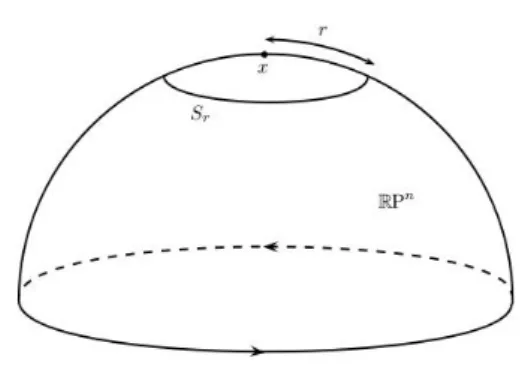
Figure 1: The equation x2

1+· · ·+x2n = (tanr)2x20 defines in RP

n

a metric sphere of radius r, i.e. the set of all points at distance r from a fixed point.

Remark. After this result was obtained P. Bürgisser has pointed out to us that it can be also derived using a limiting argument from [5], where the tube neighborhood around Ωk(X) is described.

In the case of spheres in projective space we are able to compute explicitly the volume of the manifold of tangents and hence also the expected number of flats that are simultaneously tangent to all the spheres.

Example (Spheres in projective space). Let Sri ={x

2

1+· · ·+x2n = (tanri)2x20} ⊂

RPn be a metric sphere in RPn of radius ri ∈(0, π/2), i= 1, . . . , dk,n (see Figure 1). Since all principal curvatures of Sri are constants equal to cotri and since

τk(Sr1, . . . , Sr_dk,n) =δk,n· dk,n Y i=1   2Γn+1 2 Γk+2 2 Γn−k+1 2 ·(cosri) k_(sin_r i)n−k−1  

Observe that a hypersurface Sy,r which is a sphere in some affine chart U 'Rn, i.e. Sy,r = {x∈ Rn : Pni=1(xi−yi)2 =r2}, is a convex hypersurface in RPn, but it is not a sphere with respect to the projective metric unless it’s centered at the origin (y = 0); and, viceversa, a metric sphere in _RPn needs not be a sphere in an affine chart. In fact, (5.3) tells that Sottile and Theobald’s upper bound 3·2n−1 for the number of lines tangent to d1,n affine spheres in Rn does not apply to the case

(20)

consequence there must be a configuration of d1,n projective spheres in RPn with (exponentially) more common tangent lines.

Remark (The semialgebraic case). The theorem above remains true in the case of semialgebraic hypersurfaces X1, . . . , Xdk,n ⊂ RP

n _{satisfying some mild} non-degeneracy conditions (see Section 5.5 for more details). Specifically it still holds true that τk(X1, . . . , Xdk,n) =δk,n· dk,n Y i=1 |Ωk(Xi)| |Sch(k, n)|,

but the volume of the manifold of k-tangents has a more complicated description:

|Ωk(X)| |Sch(k, n)| = _n₋₁ k Γk+1 2 Γn−k 2 πn+12 Z XEΛ∈Grk(TxX) |Bx(Λ)|dVX,

where |Bx(Λ)| denotes the absolute value of the determinant of the matrix of the second fundamental form of X ,→_RPn restricted to Λ∈Grk(TxX) and written in an orthonormal basis of Λ (see Subsection 5.2.1), and the expectation is taken with respect to the uniform distribution on Grk(TxX)'Gr(k, n−1).

The quantities|Ωk(X)|offer an alternative interesting interpretation of the

clas-sical notion of intrinsic volumes. IfC is a convex set in_RPn, the spherical Steiner’s formula [38, (9)] allows to write the volume of the -neighborhood U_RPn(C, ) of C

in_RPn as |U_RPn(C, )|=|C|+ n−1 X k=0 fk()|Sk||Sn−k−1|Vk(C), where fk() = Z 0 (cost)k(sint)n−1−kdt.

The quantities V0(C), . . . , Vn−1(C) are called intrinsic volumes of C. What is remarkable is that when C is smooth and strictly convex, |Ωk(∂C)| coincides, up

to a constant depending on k and n only, with the (n−k−1)-th intrinsic volume of C (again this property can be derived by a limiting argument from the results in [5]).

Proposition (The manifold of k-tangents and intrinsic volumes). Let C ⊂ _RPn

be a smooth strictly convex set. Then

|Vn−k−1(C)|= 1 4 ·

|Ωk(∂C)|

(21)

This interpretation offers possible new directions of investigation and allows to prove the following universal upper bound (see Corollary 9 from Chapter 5)

τk(X1, . . . , Xdk,n)≤δk,n·4

dk,n_,

where the right-hand side depends only on k and n. However, already for n = 3, as observed by T. Theobald [84] there is no upper bound on the number of lines that can be simultaneously tangent to four convex hypersurfaces in_RP3 in general position (see Section 5.4 for a proof of this fact).

Part of the results presented in the dissertation are obtained in collaboration of the author with other people: Chapter 3 is based on the joint work [21] with Paul Breiding and Antonio Lerario, the results of Chapter 4 are presented in the joint work [15] with Carlos Beltrán and Chapter 5 is a result of the joint work [52] with Antonio Lerario. In all mentioned works the contribution of the authors was comparable or equal.

(22)

Chapter 1 Notations and preliminary results

In this chapter we set our notations, give main definitions, state some classical results about spherical harmonics and semialgebraic sets and define the probabilistic framework for Chapters 3, 4 and 5.

1.1 Spherical harmonics

Let us denote by Pd,n the set of real homogeneous polynomials of degree d in n

variables x1, . . . , xn. It is a real vector space of dimension

dim(Pd,n) = n+d−1 d ! Denote by Hd,n = ( h=f|Sn−1 :f ∈ P_d,n, ∆f = ∂2f ∂x2 1 +· · ·+ ∂ 2_f ∂x2 n = 0 )

the space of restrictions to the sphere Sn−1 _{of harmonic polynomials of degree} _d_. Functions inHd,n are called spherical harmonics and the dimension of Hd,n equals

dimHd,n = n+d−1 d ! − n+d−3 d−2 ! if d≥2, dimH0,n = 1, dimH1,n =n

Definition 1. The spherical Laplace operator ∆Sn−1 is defined as follows. If

f ∈C2(Sn−1)is aC2-differentiable function onSn−1 andf˜its degree0homogeneous extension to _Rn\ {0} , i.e., f˜(x) = f(x/kxk), x∈_Rn_{\ {0}}_{, then}

(23)

Using spherical coordinates it is straightforward to check that any spherical harmonic h ∈ Hd,n is an eigenfunction of the spherical Laplace operator ∆Sn−1

corresponding to the eigenvalue−d(d+n−2). Remarkably, ∆_Sn−1 has no other

eigenfunctions [76, Thm. 22.1].

Let us now consider the standard action of the orthogonal group SO(n) on the space C(_Rn_{) of continuous functions on}

Rn:

g ∈SO(n), f ∈C(_Rn)7→f◦g−1

Since this action commutes with the Laplace operator:

∆f◦g−1 = ∆(f ◦g−1), f ∈C(_Rn), g ∈SO(n)

the space of harmonic homogeneous polynomials of degree d is invariant under it and hence the spacesHd,n, d≥0 of spherical harmonics are finite-dimensional

representations of SO(n). It turns out that these representations are actually irreducible [35, Thm. 9.3.4].

There is a special family of orthogonal polynomials that is intimately related to spherical harmonics.

Definition 2 (Gegenbauer polynomials). Let n ≥2. Gegenbauer polynomials of parameter n−₂2 are defined via the recurrence relation [2, 22.4.2, 22.7.3]:

G0,n(x) = 1, G1,n(x) = (n−2)x, Gd,n(x) = 1 d 2x(d+n 2 −2)Gd−1,n(x)−(d+n−4)Gd−2,n(x)

The polynomials {Gd,n}d≥0 form an orthogonal family on the interval [−1,1] with respect to the measure (1−z2₎n−₂3 _dz _{[2, 22.2.3]:}

1 Z −1 Gd1,n(z)Gd2,n(z) (1−z 2₎n−₂3_dz _{= 0}_, _d 1 6=d2

For any point y ∈ Sn−1 and any d ≥ 0 there exists a spherical harmonic

Z_dy ∈ Hd,n, called zonal, which is invariant under the rotations preserving y: Z_dy(g−1x) = Z_dy(x), g ∈SO(n), gy =y

The function Z_dy(x) is determined uniquely up to a constant and it is proportional to Gd,n(hx, yi) [81, Thm. 2.14],1 where hx, yi=x1y1+· · ·+xnyn is the standard

scalar product in _Rn.

1_{According to the usual definition [81, page 143] a zonal harmonic}_Zy

d is determined uniquely

by some normalization condition. Since a normalization is unimportant for our purposes we abuse the terminology and call zonal any spherical harmonic with the mentioned invariance property.

(24)

The inclusion map

i:Pd,n,→ Pd,n+1

f 7→i(f)(x1, . . . , xn, xn+1) =f(x1, . . . , xn)

induces the linear inclusion

ˆ

:Hd,n ,→ Hd,n+1

h=f|Sn−1 7→ˆh=i(f)|_Sn

We call tesseral any spherical harmonic of the form ˆh∈ Hd,n+1 for some h∈ Hd,n.

1.2 Semialgebraic geometry

The material of this section is covered by [18, 27].

Definition 3. A subset S⊂_Rn _is _{semialgebraic}_{if it can be written as} S = s [ i=1 ri \ j=1 {x∈_Rn:fi,j∗i,j0},

where fi,j ∈R[x1, . . . , xn] are some real polynomials and ∗i,j is either< or = for i= 1, . . . , s, j = 1, . . . , ri.

Remark 1. If S ⊂ _Rn _{is algebraic, i.e.,} _S ₌ _{_x _∈

Rn : f(x) = 0 ∀f ∈ B} for

some set of real polynomials B ⊂_R[x1, . . . , xn], then it is also semialgebraic since by Hilbert’s basis theorem S can be defined by a finite collection of polynomials.

Note that, by definition, the family of semialgebraic subsets of _Rn _{is closed}

under taking finite intersections, finite unions and complements and the product

S1× · · · ×Sr⊂Rn1 × · · · ×Rnr of semialgebraic subsetsSi ⊂Rni, i= 1, . . . , r is

as well semialgebraic. On of the most important statements about semialgebraic sets is Tarski-Seidenberg theorem.

Theorem 1 (Tarski-Seidenberg). If S ⊂_Rn _{is semialgebraic and} _π_:

Rn→Rk is

the projection on the first k coordinates, then π(S)⊂_Rk _{is semialgebraic.}

Morphisms between semialgebraic sets are defined as follows. Definition 4. LetS ⊂_Rn_and_T _⊂

Rk be semialgebraic sets. A mappingf :S→T

is said to be semialgebraicif its graph

Γf ={(x, y)∈S×T :f(x) =y} is a semialgebraic subset of _Rn_×

(25)

Tarski-Seidenberg theorem implies that the direct image and the inverse image of a semialgebraic set under a semialgebraic mapping are semialgebraic.

It is easy to describe the semialgebraic subsets of _R: they are the unions of finitely many points and open intervals. The following proposition asserts that as in the casen = 1 semialgebraic subsets of_Rn are nothing but finite unions of open “cubes” of different dimensions.

Proposition 1. Every semialgebraic subset S ⊂ _Rn _{can be represented as the} disjoint union S = tr

i=1Ci of a finite number of semialgebraic subsets Ci (called cells), where each cell Ci is a smooth submanifold of Rn semialgebraically dif-feomorphic to an open cube (0,1)di_{, d}

i ∈ N (with (0,1)0 being a point). The number di is the dimension of the cell Ci and the dimension of S is defined as

dim(S) = max{di :i= 1, . . . , r}. This definition does not depend on a particular decomposition of S.

Given a semialgebraic setS ⊂_Rn_{of dimension}_k _≤_n_{and given a decomposition}

ofS into cells (as in Proposition 1) we denote byStop the union of allk-dimensional cells and bySlowthe union of the cells of dimension less thank. The setsStop, Slow⊂

Rn are semialgebraic and Stop is a smooth k-dimensional submanifold ofRn. One of the central results about semialgebraic mappings is Hardt’s theorem. Theorem 2 (Hardt’s semialgebraic triviality). Let S ⊂_Rn _{be a semialgebraic set} and let f : S → _Rk _{be a continuous semialgebraic mapping. Then there exists} a finite partition of _Rk _{into semialgebraic sets} _T

1, . . . , Tr ⊂ Rk such that f is semialgebraically trivial over each Ti, i.e., there are a semialgebraic set Fi and a semialgebraic homeomorphism hi :f−1(Ti)→Ti×Fi such that the composition of hi with the projection Ti×Fi →Ti equals f|f−1₍_T

i).

The following corollary of Hardt’s theorem is frequently used to estimate dimensions of semialgebraic sets.

Corollary 1. Let S ⊂ _Rn _and _f _: _S _→

Rk be as in Theorem 2. Then the set

{x∈_Rk_{: dim(}_f−1₍_x_{)) =}_d_} _{is semialgebraic and has dimension not greater than} dim(S)−d. In particular, dim(f(S))≤dim(S).

The classical Sard’s theorem asserts that the set of critical values of a smooth mapping between two smooth manifolds is of measure zero. Its semialgebraic version allows to say a bit more.

Theorem 3 (Semialgebraic Sard’s theorem). Let f :S →T be a smooth semialge-braic mapping between smooth semialgesemialge-braic sets. Then the set of its critical values is a semialgebraic subset of T of dimension strictly less than dim(T).

(26)

1.3 Probabilistic framework

In this section we set up the probabilistic framework we will work in.

1.3.1 Conventions on metrics and volumes

The real projective space _RPn−1 is endowed with the Riemannian metric with respect to which the double coveringSn−1 2:1_−→

RPn−1 is a local isometry, where the

unit sphere Sn−1 _⊂

Rn inherits its metric from the Euclidean space Rn. We refer

to this Riemannian metric on_RPn−1 as “projective metric” or “standard metric”. The Grassmannian manifold Gr(k, n) of k-planes in _Rn _{is endowed with an} O(n)-invariant Riemannian metric through the Plücker embedding

i:Gr(k, n),→P k ^ Rn ! where P(Vk

Rn), the projectivization of the vector space VkRn 'R( n

k), is endowed

with the standard metric. Using the Plücker embedding we locally identifyGr(k, n) with the set of unit simple k-vectors v1∧ · · · ∧vk, where v1, . . . , vk are orthonormal

in_Rn _{(see [53] for more details).}

A canonical left-invariant metric on the orthogonal group O(n) is defined as

hA, Bi:= 1 2tr(A

t_B₎_{, A, B} _∈_T

1O(n)

Denoting by |M| the total volume of a Riemannian manifold M (whenever it is finite) one can prove the following formulas:

|Gr(k, n)|= |O(n)| |O(k)||O(n−k)|, |O(n+ 1)| |O(n)| =|S n_|_, _|_O_(1)|_{= 2}_, _|_Sn_|₌ 2π n+1 2 Γ(n+1₂ ).

We will also need a notion of the volume of a semialgebraic set.

Definition 5 (Volume of a semialgebraic set). Let S ⊂ _Rn _{be a semialgebraic} subset of dimension k ≤ n and Stop be the union of all k-dimensional cells of

some cell decomposition of S (see Proposition 1). The k-dimensional manifold Stop

inherits a Riemannian structure from _Rn _{and by} _|_S_|_:=_|_S

top|we denote the volume

of Stop.

One can check that this definition is independent of a particular cell decomposi-tion of the semialgebraic subsetS ⊂_Rn_.

(27)

Given a Riemannian manifold M and a measurable function f : M → _R on it we denote by R

Mf(y)dVM the integration off with respect to the Riemannian

volume density of M. We recall that there is a unique O(n)-invariant probability distribution onO(n), Gr(k, n) andSn _called_uniform _{(see [24, 53] for more details).}

For a measurable subset A⊂M ∈ {O(n), Gr(k, n), Sn}it is defined as

P(A) := 1 |M| Z M 1AdVM.

Remark 2. For a measurable A⊂Gr(k, n) the set Aˆ={g ∈O(n) :g−1_Rk ∈A}

is measurable in O(n) and P(A) = _| 1 Gr(k, n)| Z Gr(k,n) 1AdVGr(k,n) = 1 |O(n)| Z O(n) 1_AˆdVO(n)=P( ˆA)

We will implicitly use this identification when needed.

1.3.2 Integral geometry formula

The classical Poincaré’s integral geometry formula allows to compute the average number of intersection points of two planar curves, where one is fixed and the other is moved around the plane _R2 _{by a randomly chosen isometry of the plane.} Theorem 4 (Poincaré formula). Let c0, c1 ⊂R2 be two smooth planar curves and

let the isometry group I(_R2_{) =}_SO₍₂₎

o R2 of the plane be endowed with the product

Riemannian structure. Then

Z

g∈I(R2)

#(c0∩gc1)dVI(R2) = 4|c0||c1|

There are generalizations due to Brothers [22] and Howard [45] of Poincaré formula to the case of two submanifolds in an arbitrary homogeneous space endowed with an invariant metric. In Chapters 3 and 4 we will only need a version of this formula (that we state below) for submanifolds of spheres and real projective spaces and in Chapter 5 a generalized Poincaré formula for hypersurfaces in Grassmannian from [24] will be used (for this see Section 5.1).

Theorem 5 (Poincaré formula for submanifolds of a sphere). Let M, N ⊂Sn be smooth submanifolds of the sphere of dimensions dim(M) =m,dim(N) =k and let m+k ≥ n. Then for almost all g ∈ SO(n+ 1) the intersection M ∩gN is transverse and 1 |SO(n+ 1)| Z g∈SO(n+1) |M ∩gN|dVSO(n+1) =|Sm+k−n| |M| |Sm_| |N| |Sk_|

(28)

The above formula also holds in case when M, N ⊂Sn _{are algebraic subsets (even} singular).

The following corollary of Theorem 5 will be particularly useful for us.

Corollary 2. Let M ⊂_RPn be a smooth submanifold of dimension dim(M) = m, N '_RPk⊂_RPn be a k-dimensional projective subspace and let m+k ≥n. Then for almost all g ∈SO(n+ 1) the intersection M∩gN is transverse and

EL∈G(k,n)|M ∩L|= 1 |SO(n+ 1)| Z g∈SO(n+1) |M ∩gN|dVSO(n+1) =|RPm+k−n| |M| |_RPm|,

where_G(k, n)'Gr(k+1, n+1)denotes the Grassmannian of projectivek-subspaces in_RPn. Again, the above formula also holds in case whenM ⊂_RPn is an algebraic subset (even singular).

1.3.3 Smooth coarea formula

Let f :M →N be a smooth map between two smooth manifolds. A point x∈M

is called a regular point of f if the differential Dxf :TxM →Tf(x)N is surjective, otherwise x ∈ M is called a critical point. The point y ∈ N is called a regular value of f if its preimagef−1₍_y_{) consists only of regular points, otherwise} _y_∈_N _is called a critical value. By convention, any point y∈N \f(M) outside the image of f is a regular value. Note that if dim(M)<dim(N), then all pointsx∈M are critical for f.

Sard’s theorem asserts that the set of critical values of f has zero measure. Let now f :M →N be a smooth map between two Riemannian manifolds of dimensions dim(M) =m,dim(N) =k.

Definition 6. The normal Jacobian N Jxf of f at x∈M is defined as follows. If x∈M is a critical point of f then N Jxf = 0, otherwise

N Jxf =kDxf(e1)∧ · · · ∧Dxf(ek)k,

where e1, . . . ek∈(ker(Dxf))⊥ is any orthonormal basis of the orthogonal comple-ment to the kernel of the differential of f at x.

The smooth coarea formula is a far going generalization of the classical formula for the change of variables in the integral.

(29)

Theorem 6 (Smooth coarea formula). Let f :M →N be a smooth map between Riemannian manifolds of dimensions dim(M) = m,dim(N) =k. Then

Z y∈N Z x∈f−1₍_y₎ h(x)dVf−1₍_y₎dV_N = Z x∈M h(x)N Jxf dVM

for any Borel measurable function hdefined almost everywhere on M and such that the integral on the right is finite.

Remark 3. Note that when almost all points x∈M are regular one can rewrite the smooth coarea formula as follows:

Z y∈N Z x∈f−1₍_y₎ h(x)(N Jxf)−1dVf−1₍_y₎dV_N = Z x∈M h(x)dVM

1.3.4 Random matrices

The space M(n,_R) of n×n real matrices is endowed with the Frobenius inner product and the associated norm:

(A, B) = tr(AtB), kAk2 _{= (}_{A, A}₎_, _{A, B} _∈_M₍_n,

R).

Any k-dimensional vector subspace V ⊂ M(n,_R) is endowed with the standard normal probability distribution NV:

PNV(U) = 1 √ 2πk Z U e−kvk 2 2 dv,

wheredv is the Riemannian volume density on (V,(·,·)) andU ⊂V is a measurable subset.

In case when V = Sym(n,_R) is the space of real symmetric n×n matrices the probability space (Sym(n,_R),NSym(n,R)) is calledthe Gaussian Orthogonal Ensemble

and random matrices taking values in it are called GOE(n)-matrices. Denoting by dQ=Q

1≤i≤j≤ndQij the Lebesgue measure of the entries of a symmetric matrix Q∈Sym(n,_R) one can write

PGOE(n){U}= 1 √ 2n√πN Z U e−kQk 2 2 dQ,

where N = dim(Sym(n,_R)) = n+1₂ and U ⊂ Sym(n,_R) ' _RN _{is a measurable}

(30)

orthogonal matrices, the GOE(n) measure on Sym(n,_R) induces a probability measure on the space of eigenvalues _Rn [63, Sect. 3.1]:

P{U}:= 1 Zn Z U e−kλk 2 2 |∆(λ)|dλ wheredλ=Qn

i=1dλi is the Lebesgue measure onRn,U ⊂Rnis a measurable subset,

kλk2 ₌_λ2

1+· · ·+λ2n is the Euclidean norm ofλ ∈Rn, ∆(λ) :=

Q

1≤i<j≤n(λj −λi)

is the Vandermonde determinant andZn is the normalization constant. The value

of Zn equals [63, (17.5.9)] Zn:= Z Rn e−kλk 2 2 |∆(λ)|dλ= √ 2πn n Y i=1 Γ(1 + ₂i) Γ(3₂) (1.1)

The unit sphere SN−1 _:= _{_Q_∈ _Sym(_n,

R) :kQk= 1} in the space of symmetric

matrices is endowed with the uniform measure. Then the normalized volume |E|/|SN−1_| _{of any measurable set} _E _⊂ _SN−1 _{equals the GOE(}_n_{) measure of the} cone C(E) :={Q∈Sym(n,_R) :Q/kQk ∈E} overE:

|E|

|SN−1_| =P{C(E)} (1.2) This property of the GOE measure will be useful for us.

(31)

Chapter 2 Spherical harmonics with the

maximum number of critical

points

Spherical harmonics are the restrictions to the standard unit sphere of harmonic homogeneous polynomials. They can be equivalently defined as eigenfunctions of the spherical Laplace operator. Spherical harmonics play an important role in mathematics (the theory of special functions, spectral geometry) and physical sciences (quantum mechanics, cosmology, geodesy).

The study of geometric and topological properties of Laplace eigenfunctions on Riemannian manifolds has rich and interesting history, we refer the reader to the survey of the results [89]. Being eigenfunctions of the spherical Laplace operator spherical harmonics have many remarkable properties that are not shared by general homogeneous polynomials. For example, the algebraic hypersurface they define cannot have arbitrarily small volume. In fact, from the result [30, Thm. 1.2] of Donnelly and Fefferman it follows that if h ∈ Hd,n+1 is a spherical harmonic corresponding to a harmonic homogeneous polynomial of degreedinn+ 1 variables then the (n−1)-dimensional Hausdorff volume of the nodal hypersurface Nh ={x∈Sn :h(x) = 0} of the spherical harmonich satisfies

cn

q

λd,n ≤Hn−1(Nh),

wherecn >0 is a positive constant that depends only onnand−λd,n= −d(d+n−1) is the eigenvalue of the spherical Laplace operator ∆Sn that corresponds to h.

Another interesting result concerns topological properties of nodal sets of spherical harmonics. Connected components of the complement in the sphere to the nodal hypersurface of a spherical harmonic are called nodal domains. In [67] Pleijel proved the following asymptotic bound on the numberµ(h) of nodal domains

(32)

inS2 _{of a spherical harmonic} _h_{∈ H} d,3: lim d→+∞ µ(h) d(d−1) <0.69 (2.1) By the results of Harnack [42] a real plane algebraic curve of degree d, i.e., the zero set in _RP2 of a real homogeneous polynomial of degree d, cannot have more than (d−1)(d−2)/2 + 1 connected components in _RP2 when it is non-singular and this bound is attained by some non-singular curves which are calledM-curves. The result (2.1) in particular implies that the non-singular real plane algebraic curves defined by harmonic homogeneous polynomials cannot be M-curves (at least when the degree d is large enough). In [11, Problem 1] Arnold asked to determine for a given d the maximum number of nodal domains that a spherical harmonic

h∈ Hd,3 can have. In [56] trying to answer Arnold’s question Leydold conjectured the following formula:

max h∈Hd,3 µ(h) =    1 2(d+ 1) 2_, _if _d _{is odd} 1 2d(d+ 2), if d is even

and he proved it for d≤6. For d >6 the problem is still open to our knowledge. Also in [11, Problem 1] Arnold asked to determine the largest number of local maxima that a Morse spherical harmonich∈ Hd,3 can have on the sphere S2. For even d the answer to this question is not known in general (to our knowledge). For odd dthe answer (d2₋_d_{+ 2)}_/_{2 was given by Kuznetsov and Kholshevnikov in [54],} where they also proved that the maximum number md,3 of critical points of the restrictionf|_S2 to the sphere of a Morse (see Subsection 2.1.1) real homogeneous

polynomial f ∈ Pd,3 of degreed equals:

md,3 = 2(d2−d+ 1)

and surprisingly enough this bound is attained by spherical harmonics. In the following theorem we generalize the result of Kuznetsov and Kholshevnikov to the case of any number of variables.

Theorem 7. For any d≥1andn ≥2the maximum numbermd,n of critical points of the restriction f|Sn−1 to the sphere of a Morse real homogeneous polynomial

f ∈ Pd,n of degree d equals

md,n = 2

(d−1)n−1

d−2 = 2((d−1)

n−1₊_{· · ·}_{+ (}_d₋_{1) + 1)}

Moreover, for anyd≥1andn ≥2there exist a Morse spherical harmonich∈ Hd,n with md,n critical points.

Extremal and typical results in Real Algebraic Geometry

Scuola Internazionale Superiore di Studi Avanzati

Area of Mathematics