A Mathematical Formalization of Hierarchical Temporal Memory\u27s Spatial Pooler for use in Machine Learning

(1)

Rochester Institute of Technology

RIT Scholar Works

Theses Thesis/Dissertation Collections

4-15-2016

A Mathematical Formalization of Hierarchical

Temporal Memory's Spatial Pooler for use in

Machine Learning

James W. Mnatzaganian

[email protected]

Follow this and additional works at:http://scholarworks.rit.edu/theses

This Thesis is brought to you for free and open access by the Thesis/Dissertation Collections at RIT Scholar Works. It has been accepted for inclusion in Theses by an authorized administrator of RIT Scholar Works. For more information, please [email protected].

Recommended Citation

Mnatzaganian, James W., "A Mathematical Formalization of Hierarchical Temporal Memory's Spatial Pooler for use in Machine Learning" (2016). Thesis. Rochester Institute of Technology. Accessed from

(2)

A Mathematical Formalization of

Hierarchical Temporal Memory’s Spatial Pooler

for use in Machine Learning

(3)

A Mathematical Formalization of

Hierarchical Temporal Memory’s Spatial Pooler

for use in Machine Learning

James W. Mnatzaganian April 15, 2016

A Thesis Submitted in Partial Fulfillment

of the Requirements for the Degree of Master of Science

in

Computer Engineering

(4)

A Mathematical Formalization of

Hierarchical Temporal Memory’s Spatial Pooler

for use in Machine Learning

James W. Mnatzaganian

Committee Approval:

Dr. Dhireesha Kudithipudi Advisor Date

Associate Professor

Dr. Ernest Fokou´e Date

Associate Professor

Dr. Andreas Savakis Date

(5)

To my loving wife, Haley.

Thank you for believing in me, and being there with me through the thick of it all. I love you.

(6)

Acknowledgments

I firstly and formally am thankful for my heavenly father. This work would not have been possible without His gracious hand guiding me all the way. John 14:14 (NIV) “You may ask me for anything in my name, and I will do it.”

I am grateful for my advisor, Dr. Dhireesha Kudithipudi. Thank you for your guidance and support. I was truly grateful to have you as my advisor.

I am thankful for my committee members Dr. Ernest Fokou´e and Dr. Andreas Savakis. Thank you Dr. Fokou´e for the mathematical support. Thank you Dr. Savakis for your time, and for helping keep my expectations realistic.

I am thankful for our research team at the NanoComputing Research Lab. All of you have helped me more than you will ever realize. James Thesing, thank you for all of the times you diligently listened to me, and for your input. Levs Dolgovs, thank you for our late night discussions. Qutaiba Saleh, thank you for our discussions. Dr. Cory Merkel, thank you for your general help on everything. Amanda Hartung, thank you for your extreme diligence – keep up the good work! Lennard Streat thanks for all of the HTM input. Everyone else who I did not mention, thank you all for your general friendship and support. This truly was a team effort!

I am very thankful for the staff at RIT’s research computing. Without their support and the use of their equipment, my experiments would still be running!

I am thankful for Kevin Gomez of Seagate Technology for his support. I am thankful for the Numenta team for their input.

I am also thankful for my friends that provided help and support. In particular, Matthew Filmer – Thanks for reminding me that MS ! = PhD and for the LA_{TEX help.} Lastly, I am extremely grateful for my family. Without all of you keeping me straight, my head would have come off!! I love you all dearly. You have all supported me and believed in me from the beginning. Thank you for not only tolerating me, but showing me much love, during my season of business.

(7)

Abstract

Hierarchical temporal memory (HTM) is an emerging machine learning algorithm, with the potential to provide a means to perform predictions on spatiotemporal data. The algorithm, inspired by the neocortex, consists of two primary components, namely the spatial pooler (SP) and the temporal memory (TM). The SP is utilized to map similar inputs into generalized sparse distributed representations (SDRs). Those SDRs are then utilized by the TM, which performs sequence learning and prediction. One challenge with HTM is ensuring that proper SDRs are generated from the SP. If the SDRs are not generalizable, the TM will not be able to make proper predictions. This work focuses on the SP and its corresponding output SDRs. A single unifying mathematical framework was created for the SP. The primary learning mechanism was explored, where a maximum likelihood estimator for determining the degree of permanence update was proposed. The boosting mechanisms were studied and found to only be relevant during the initial few iterations of the network. Observations were made relating HTM to well-known algorithms such as competitive learning and attribute bagging. Methods were provided for using the SP for classification as well as dimensionality reduction. Empirical evidence verified that given the proper pa-rameterizations, the SP may be used for feature learning.

Similarity metrics were created for scoring the SDRs produced by the SP. The overlap metric proved that the SP is extremely robust to noise. The SP was able to produce similar outputs for a given input, provided the noise did not cause the input to change classes. This overlap metric was further utilized to create a classifier for novelty detection. The SP proved to be able to withstand more noise than the well-known support vector machine (SVM).

(8)

List of Figures

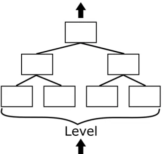
2.1 Example SDR encoding for the days of the week. In this example, Sunday is similar to both Saturday and Monday, denoting a periodic pattern. . . 7 2.2 A generic HTM, consisting of three levels. The first level is at the

bottom of the hierarchy and the last level is at the top of the hierarchy. The inputs are fed bottom-up, with the final output produced from the last level. . . 8 3.1 An HTM consisting of three levels. The first level is at the bottom

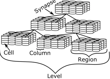
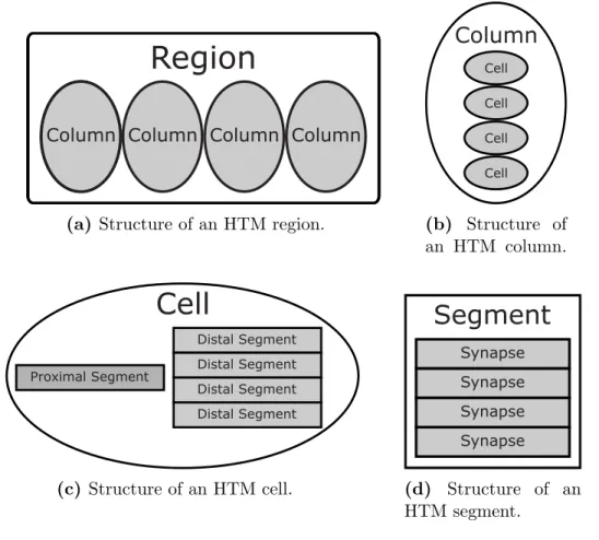
of the hierarchy and the last level is at the top of the hierarchy. The inputs are fed bottom-up, with the final output produced from the last level. Each level contains one or more regions comprised of columns of cells. Connections between cells, within a region, also occur. . . 12 3.2 Structure of the various components inside of an HTM. A region (a) is

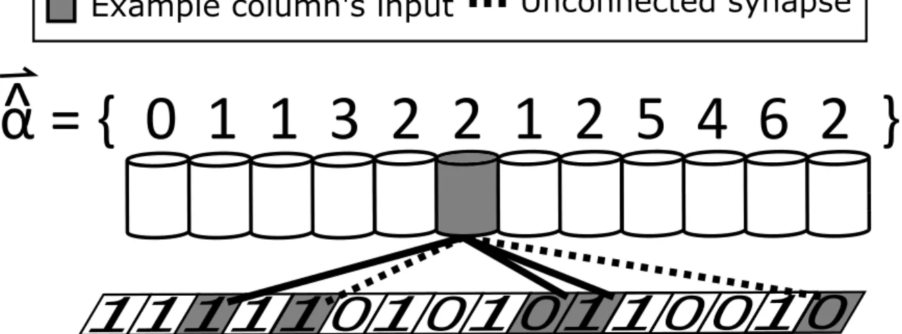
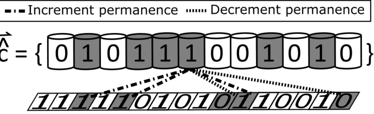
comprised of columns (b) of cells (c) of segments (d) of synapses. There may exist multiple types of each subcomponent, except the proximal segment, which is limited to one per column. . . 13 4.1 SP phase 1 example wherem = 12,q = 5, andρd= 2. It was assumed

that the boost for all columns is at the initial value of ‘1’. For simplicity, only the connections for the example column, highlighted in gray, are shown. . . 28 4.2 SP phase 2 example whereρc= 2 andσo = 2. The overlap values were

determined from the SP phase 1 example. . . 29 4.3 SP phase 3 example, demonstrating the adaptation of the permanences.

The gray columns are used denote the active columns, where those activations were determined from the SP phase 2 example. . . 31 4.4 Demonstration of boost as a function of a column’s minimum active

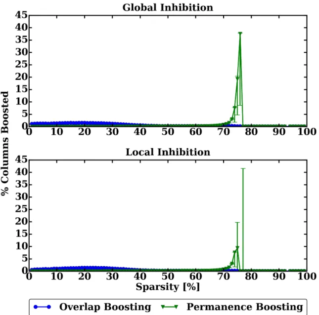
duty cycle and active duty cycle. . . 35 4.5 Demonstration of frequency of both boosting mechanisms as a

func-tion of the sparseness of the input. The top figure shows the results for global inhibition and the bottom figure shows the results for local inhibition1_. _{. . . .} ₃₆

(12)

LIST OF FIGURES

4.6 Frequency of boosting for the permanence boosting mechanism for a sparsity of 74%. The top figure shows the results for global inhibi-tion and the bottom figure shows the results for local inhibiinhibi-tion Only the first 200 iterations were shown, for clarity, as the remaining 800 propagated the trend. . . 37 5.1 Scalar encoding example demonstrating the cases without (a) and with

wrapping (b). For both cases, four active bits and three bins were used with the bin overlap set to 70%. The encoding bounds are zero and two for the minimum and maximum, respectively. . . 46 5.2 Depiction of a multivariate encoder withn encoders. . . 48 5.3 Procedure for classifying with a single SP. . . 49 5.4 Reconstruction of the input from the context of the SP. Shown are

the original input images (top), the sparse distributed representations (middle), and the reconstructed version (bottom). . . 56 6.1 Uniqueness metric on SPD for varying degrees of noise. . . 62 6.2 Overlap metric on SPD for varying degrees of noise. . . 64 6.3 Novelty detection, training, results for the SP (a) and the SVM (b). . 68 6.4 Restricted version of Figure 6.3b, where the noise ranged between 5

and 95%. . . 69 6.5 Novelty detection, testing, results for the SP (a) and the SVM (b). . . 70 6.6 Novelty detection results for non-overlapping inputs. The training (a)

and the testing (b) results are shown.

. . . 73 6.7 Novelty detection results for samples generated with a noise variation

(13)

List of Tables

4.1 User-defined parameters for the SP . . . 23 5.1 SP Performance on MNIST using Global Inhibition . . . 55 5.2 SP Performance on MNIST using Local Inhibition . . . 55

(14)

List of Symbols

Term Description

∃! Uniqueness quantification.

n Number of patterns (samples).

p Number of inputs (features) in a pattern.

m Number of columns.

q Number of proximal synapses per column.

φ+ Permanence increment amount.

φ− Permanence decrement amount.

φδ Window of permanence initialization.

ρd Proximal dendrite segment activation threshold.

ρs Proximal synapse activation threshold.

ρc Desired column activity level.

κa Minimum activity level scaling factor.

κb Permanence boosting scaling factor.

β0 Maximum boost.

τ Duty cycle period.

s Integer index bounded by [0, n).

r Integer index bounded by [0, p).

i Integer index bounded by [0, m).

j Integer index bounded by [0, m).

k Integer index bounded by [0, q).

U Set of inputs for all patterns. U ∈ {0,1}n×p_.

U(tr) Set of inputs for all training patterns. U(tr) ∈ {0,1}n×p_. _n _{in this context represents the number}

of rows in U(tr).

U(te) Set of inputs for all testing patterns. U(te) ∈ {0,1}n×p_. _n _{in this context represents the number}

of rows in U(te).

W Set of SP output SDRs for all patterns. W ∈ {0,1}n×m_.

(15)

Term Description

W(tr) Set of SP output SDRs for all training patterns.

W(tr) ∈ {0,1}n×m_. _n _{in this context represents the}

number of rows in U(tr).

W(te) Set of SP output SDRs for all testing patterns.

W(te) ∈ {0,1}n×m_. _n _{in this context represents}

the number of rows in U(te).

*

c Set of all columns indices. *c∈_Z1×m_,*

c∈[0, m). Λ Source column indices for each proximal synapse on

each column. Λ∈ {r}m×q_.

Φ Set of permanences for each column. Φ∈_Rm×q_.

X Set of inputs for each column. X ∈ {0,1}m×q_.

X Overall mean of X.

*

b Set of boost values for all columns. *b∈_R1×m_.

H Neighborhood mask for all columns. H ∈ {0,1}m×m_.

Y Bit-mask for the proximal synapses’ activations.

Y ∈ {0,1}m×q_.

*

z Attribute mask. *z ∈ {0,1}1×p_.

*

α Overlap for all columns. *α∈ {0,1}1×m_.

*

ˆ

α Sum of the active connected proximal synapses for all columns. *αˆ ∈_Z1×m_.

*

γ ρc-th largest overlap (lower bounded by one) in the

neighborhood of *ci ∀i. *γ ∈Z1×m.

δΦ Proximal synapses’ permanence update amount, following the original terminology. δΦ∈_Rm×q_.

δΨ Proximal synapses’ permanence update amount, following the new terminology. δΨ∈_Rm×q_.

*

η(a) _{Set of active duty cycles for all columns.}

*

_η(a) _∈

R1×m.

*

η(o) _{Set of overlap duty cycles for all columns.}

*

_η(o) _∈

R1×m.

*

η(min) _{Set of minimum active duty cycles for all columns.}

*

η(min) _∈

(16)

Term Description

D Distance between an SP column and its correspond-ing connected synapses’ source columns. D ∈ Rm×q.

σ0 Inhibition radius.

*

ˆ

c Set of active columns. *cˆ∈ {0,1}1×m_.

*

ˆ

φ Set of learned attribute probabilities.

*

φˆ∈(0,1)1×p.

*

ˆ

u Reconstructed input. *uˆ∈ {0,1}1×p_.

ˆ

θM LE MLE of θ.

J Matrix of ones with dimensions m×q.

t Scaling factor equal to m×q.

κ Scaling parameter defined such that κ

X ∈[0,1] and

κ

1−X ∈[0,1].

θ Probability of an input being active.

*

icr Event of input r connecting to column i.

* ic ∈ {0,1}1×p_.

ACi,k Event that proximal synapse k is active and

con-nected on column i. AC ∈ {0,1}m×q_.

*

λ Random vector governing the count of connections between each input and all columns. *λ∈_Z1×p_,*_λ_∈

[0, q+m].

λ0 Random variable governing the number of uncon-nected inputs.

*

aii Random variable governing the number of active

inputs on column i. *ai∈_Z1×m_,*_ai_∈_[0_{, q}_].

a Random variable governing the average number of active inputs on a column.

*

aci Random variable governing the number of active

and connected proximal synapses for column i.

*

ac∈_Z1×m_,*

ac∈[0, q].

at Random variable governing the number of columns having at least ρd active proximal synapses.

act Random variable governing the number of columns having at least ρd active connected proximal

(17)

Term Description

πx Random variable that is equal to the overall mean

of _P(X).

πac Random variable that is equal to the overall mean

of _P(AC).

*

πw Random variable that represents the mean across

the rows of W(tr).

µu Uniqueness metric. A metric for evaluating the

quality of output SDRs of the SP. A value of zero indicates that all SDRs are identical and a value of one indicates that all SDRs are unique.

µo Overlap metric. A metric for evaluating the quality

of output SDRs of the SP. A value of one indicates that all SDRs are identical and a value of zero in-dicates that all SDRs are unique.

ao Average overlap across all pair-wise vectors in W.

mo Maximum overlap on two given vectors in W.

*

w0 Base class representation for all of the SDRs in

(18)

List of Functions

Name Description

I(k) Indicator function. Returns ‘1’ if parameter k is true and ‘0’ otherwise.

Ber Bernoulli distribution.

Bin(k;n, p) PMF of a binomial distribution, where k is the number of successes, n is the number of trials, and

p is the success probability in each trial. min(*v) Returns the minimum value in *v.

max(*v) Returns the maximum value in *v. kmax(S, k) Returns the k-th largest element of S.

clip(M, lb, ub) Clips all values in the matrix M outside of the range [lb, ub] to lb if the value is less than lb, or to

ub if the value is greater than ub.

update active duty cycle(*c) Updates the moving average duty cycle for the ac-tive duty cycle for each *ci ∈*c.

update overlap duty cycle(*c) Updates the moving overlap duty cycle for the over-lap duty cycle for each *ci ∈

* c. β

*

η(_ia),

*

η(_imin)

Updates the boost values for each *ci ∈*c.

d(x, y) Distance function. Returns the distance between x

and y.

pos(c, r) Returns the position of the column indexed at c, located r regions away from the current region. h(*ci) Neighborhood function. Returns the neighbors for

*

(19)

Acronyms

2D two-dimensional 3D three-dimensional

ANN artificial neural network API application program interface

CLA cortical learning algorithm CNN convolutional neural network CV cross-validation

HTM hierarchical temporal memory

i.i.d. independent and identically distributed

mHTM math hierarchical temporal memory MLE maximum-likelihood estimator

MNIST modified National Institute of Standards and Technology

NuPIC Numenta platform for intelligent computing

PMF probability mass function

SDR sparse distributed representation SOM self-organizing map

(20)

Acronyms

SPD spatial pooler dataset

SPNDC spatial pooler novelty detection classifier SVM support vector machine

TM temporal memory TP temporal pooler

(21)

Chapter 1 Introduction

Hierarchical temporal memory (HTM) is a machine learning algorithm that was in-spired by the neocortex and designed to learn sequences and make predictions. In its idealized form, it should be able to produce generalized representations for similar inputs. Given time-series data, HTM should be able to use its learned representations to perform a type of time-dependent regression. Such a system would prove to be incredibly useful in many applications utilizing spatiotemporal data. One instance for using HTM with time-series data was recently demonstrated by Cui et al. [1], where HTM was used to predict taxi passenger counts. The use of HTM in other applica-tions remains unexplored, largely due to the evolving nature of HTM’s algorithmic definition. Additionally, the lack of a formalized mathematical model hampers its prominence in the machine learning community. This work aims to bridge the gap between a neuroscience inspired algorithm and a math-based algorithm by construct-ing a purely mathematical framework around HTM’s original algorithmic definition. HTM models, at a high-level, some of the structures and functionality of the neocortex. Its structure follows that of cortical minicolumns, where an HTM region is comprised of many columns, each consisting of multiple cells. One or more regions form a level. Levels are stacked hierarchically in a tree-like structure to form the full network. Within HTM, connections are made via synapses, where both proximal and distal synapses are utilized to form feedforward and neighboring connections,

(22)

CHAPTER 1. INTRODUCTION

respectively.

The current version of HTM is the predecessor to HTM cortical learning algo-rithm (CLA) [2]. In the current version of HTM the two primary algoalgo-rithms are the spatial pooler (SP) and the temporal memory (TM). The SP is responsible for taking an input, in the format of a sparse distributed representation (SDR), and producing a new SDR. In this manner, the SP can be viewed as a mapping function from the input domain to a new feature domain. In the feature domain a single SDR should be used to represent similar SDRs from the input domain. The algorithm is a type of unsupervised competitive learning algorithm that uses a form of vector quanti-zation (VQ) resembling self-organizing maps (SOMs). The TM is responsible for learning sequences and making predictions. This algorithm follows Hebb’s rule [3], where connections are formed between cells that were previously active. Through the formation of those connections a sequence may be learned. The TM can then use its learned knowledge of the sequences to form predictions.

HTM originated as an abstraction of the neocortex; as such, it does not have an ex-plicit mathematical formulation. Without a mathematical framework, it is difficult to understand the key characteristics of the algorithm and how it can be realized. In gen-eral, very little work exists regarding the mathematics behind HTM. Hawkins et al. [4] recently provided a starting mathematical formulation for the TM, but no mentions to the SP were made. Lattner [5] provided an initial insight about the SP, by relating it to VQ. He additionally provided some equations governing computing overlap and performing learning; however, those equations were not generalized to account for local inhibition. Byrne [6] began the use of matrix notation and provided a basis for those equations; however, certain components of the algorithm, such as boosting, were not included. Leake et al. [7] provided some insights regarding the initialization of the SP. He also provided further insights into how the initialization may affect the initial calculations within the network; however, his focus was largely on the network

(23)

initialization. The goal of this work is to provide a complete mathematical framework for HTM’s SP. Additionally, this work aims to provide a basis for utilizing HTM’s SP in machine learning.

1.1 Research Statement and Contributions

This work was created with the belief that formalized spatiotemporal algorithms, in-spired by the neocortex, will advance the machine learning of tomorrow. As such, the primary objective of this work was to formalize the SP, and to apply that formaliza-tion in the field of machine learning.

The aforementioned formalization was created in Chapter 4. This mathematical framework took into consideration all aspects of the SP and brought them together under a single unifying framework. In addition to the primary operation of the SP, the initialization as well as the boosting mechanisms were described. The initialization work provides a probabilistic approach for determining the initial expected output of the SP; thereby, creating an easy technique for choosing suitable parameters. The model for boosting provided a premises for evaluating the effectiveness of the strategy, where it was found that the current boosting technique will typically make little difference in the SP’s learned representations.

In addition to those contributions, the framework provided a foundation for study-ing the primary learnstudy-ing mechanism of the SP. Through that study, a plausible ex-planation for the origin of the permanence update amount was created. An estimator was developed to optimize the permanence increment and decrement amounts. The SP was also described in terms of traditional machine learning algorithms, where it was found that the SP is similar to attribute bagging with a competitive learning network as the base learner.

An open-source Python implementation of the aforementioned framework was developed (see Section 5.1). This implementation of the SP was unique, because it

(24)

specifically allowed the SP to be utilized in the same manner as any other comparable machine learning algorithm. This implementation will allow future researchers to easily utilize the SP in their present or future studies.

Using the created mathematical framework and software solution, the SP was demonstrated in a number of areas within machine learning (see Section 5.4 and Section 6.2). In addition to the traditional use case of classification, the SP was used to perform feature extraction, dimensionality reduction, and novelty detection. A method was also created for using the SP’s output, along with its permanences, to recreate the input.

Two methods were created to evaluate the quality of the SP’s SDRs (see Sec-tion 6.1). Those metrics, the uniqueness metric and the overlap metric, proved to provide a suitable means for evaluating the SP’s SDRs. Additionally, those metrics were used to show that the SP is extremely robust to noise and is able to create

similar SDRs for similar inputs. The result of the latter provides confirmation that the SP algorithm is able to perform is primary goal of feature mapping.

1.2 Document Structure

Chapter 2 discusses the necessary background relating to HTM. Additional informa-tion is provided discussing the algorithm’s history. Chapter 3 provides an overview of the SP. All components utilized by the SP are explained, in their original terms. A high-level overview of the operations of the SP is provided, with corresponding pseudocode.

Chapter 4 introduces the mathematical model created for the SP. The notation utilized by this work is explained. Additionally, insights into the SP’s primary learning mechanism are provided.

Chapter 5 provides detailed instructions on how to begin using the SP for machine learning related tasks. Data encoding is explained, with details provided for various

(25)

encoders. An explanation on how to train the SP is provided. Feature learning is discussed, with a demonstration of multi-class classification.

Chapter 6 discusses how to evaluate the SDRs produced by the SP. One of the introduced metrics is used to create a classifier. That classifier is then demonstrated in the context of novelty detection.

Chapter 7 summaries this work. It also provides some final remarks regarding other aspects of the SP algorithm.

(26)

Chapter 2 Background

2.1 Memory-Prediction Framework

A theory of brain function, known as the memory-prediction framework, was devel-oped by Hawkins [8] to describe the manner in which the mammalian neocortex stores and utilizes memory. The theory proposes the notion of a single algorithm to describe the processing of all cortical information.

In this theory, a bi-directional, tree shaped hierarchy of regions are used to process data. Inputs enter at the lowest levels of the hierarchy, and information flows through the system in both a feedforward and feedback manner. In each region, an invariant representation of the information is created and stored in the form of patterns. This type of data storage is an autoassociative memory, where patterns are retrieved based on similarities to past patterns.

Each time an input is presented to the system, the current region infers as to what the input represents, passing its knowledge up the hierarchy, representing a feedforward flow. The region, storing past-occurrences of feedforward inputs, is able to combine feedback from higher levels with its memory and the current feedforward input to make a prediction about the next input.

Through the changing of input, each region is able to learn sequences of patterns. The higher regions are able to use the representations of the lower regions to learn

(27)

CHAPTER 2. BACKGROUND

Sunday : 11100000000000000000000000 Monday : 01110000000000000000000000

· · ·

Saturday : 11000000000000000000000001

Figure 2.1: Example SDR encoding for the days of the week. In this example, Sunday is similar to both Saturday and Monday, denoting a periodic pattern.

sequences of higher-order objects. This process allows higher levels to become more invariant, as less details are propagated forward through the network.

2.2 Sparse Distributed Representation (SDR)

HTM uses the concept of sparse distributed representations (SDRs), where a given input is encoded into a quantized binary representation. This binary representation has a small number of active bits. SDRs are primarily used to allow a type of similarity between inputs to occur.

For example, an SDR of the days of the week, might look something like the vectors shown in Figure 2.1. In that figure, Sunday shares two bits with Monday, implying that Sunday and Monday are similar. In this case, “similar” represents days of the week that are close in order. Additionally, Sunday shares two bits with Saturday, thus denoting a periodic pattern, as the first and last elements are similar. If the number of overlapping bits were to increase, the resolution would also in-crease, allowing for an increase in step size between encodings. Additionally, an increase in bit overlap improves the robustness of the system, as only a single bit overlap is required to classify two inputs as similar.

SDRs are utilized by an HTM in a number of places. Before an HTM is able to use input data, it must first be encoded by an appropriate encoder (see Section 5.2 for more details). The encoder is used to map the input from its current form into its corresponding SDR form. While encoders are not explicitly part of an HTM they are a necessary requirement for the system.

(28)

Level

Figure 2.2: A generic HTM, consisting of three levels. The first level is at the bottom of the hierarchy and the last level is at the top of the hierarchy. The inputs are fed bottom-up, with the final output produced from the last level.

Within an HTM, SDRs are used whenever data is stored or read. This most prominently appears as an output from the SP, the current state of the TM, and a prediction from the TM.

2.3 Hierarchical Temporal Memory (HTM)

Hierarchical temporal memory (HTM) is a machine learning algorithm, created by Hawkins and George [9] that is based on the memory-prediction framework. A basic depiction of the system is shown in Figure 2.2. That system is comprised of three levels. The inputs to the network are fed bottom-up from level one up through level three. The overall output of the system is produced at the last level.

Originally, HTM, was developed as a system capable of performing invariant visual pattern recognition [10]. That version of HTM, known as Zeta 1, was built upon a Bayesian framework. After Zeta 1, Zeta 2 was developed.

The Zeta algorithms were succeeded by the cortical learning algorithms (CLAs). The CLAs were defined to be a category of algorithms utilized in HTM, explicitly

(29)

known as the HTM CLAs [2]. The CLAs were comprised of the spatial pooler (SP) and the temporal pooler (TP). Following HTM CLA came the current version of HTM, which is simply known as HTM [4]. This version of HTM is similar to HTM CLA, with the most noticeable difference being that the TP is replaced by tempo-ral memory (TM).

HTM is under active development and as such, its details are changing. For purposes of clarity, this work primarily follows the definitions from the original HTM CLA whitepaper [2]. To ensure that the most recent details are provided, the latest version of HTM was used as a reference. All areas of ambiguity are explained as they appear. Terminology is used to follow the current version of HTM, to help remove any future confusion.

2.3.1 Zeta Algorithms

Zeta 1 HTM refers to the HTM described in [10]. This type of HTM is constructed with nodes. Each box in Figure 2.2 represents a node, with multiple nodes comprising a level. The nodes are the basic building blocks of Zeta 1 HTM and include both the algorithmic and memory components of the system. Nodes are used to learn spatial invariant representations of input spaces.

The nodes have two phases of operations. The first phase, learning, is where the node creates internal representations of the input. The second phase, sensing / infer-ence, is where the node produces an output for the input. During the learning phase, three operations occur: memorization of patterns, learning transition probabilities, and temporal grouping. In this context, a “pattern” refers to the input the node receives at a given instance, in time.

During the memorization phase, unique occurrences of each pattern are labeled and stored. During the learning transition probabilities phase, a Markov chain is maintained. Each vertex in the chain corresponds to a stored pattern. The link

(30)

between two vertices corresponds to the probability of the pattern occurring. The probability is simply a unity normalized value corresponding to the percentage the transition from one pattern to another pattern occurred.

During the temporal grouping phase, patterns are clustered using agglomerative hierarchical clustering. Each cluster in the hierarchical clustering dendrogram cor-responds to a set of patterns that are likely to follow one another, in time. Those clusters are known as temporal groups.

Once the learning phase has completed, the sensing / inference phase may occur. In this phase, each node produces an output based on an instantaneous input. The closeness of the input pattern to the patterns stored in memory is calculated. The closeness is measured by the Euclidean distance between all vertices in a temporal group. The node’s output is a unity normalized vector containing the probabilities of the input pattern matching each temporal group.

(31)

Chapter 3 Spatial Pooler (SP) Overview

HTM is comprised of multiple levels, with each level consisting of one or more regions. The term level refers to the HTM’s structure, where a level contains all components within a single rank of the hierarchy. A region refers to the functionality within the level. Each region is comprised of one or more columns consisting of one more cells. The cells act as the fundamental functional unit within an HTM. An example HTM architecture is depicted in Figure 3.1. This chapter explains those individual components, as well as the spatial pooler (SP) and its role within HTM.

3.1 HTM Components

An HTM is comprised of a number of components, many of which follow a naming convention inspired from neuroscience. Structurally, an HTM is a tree-shaped hierar-chy of levels. Each level consists of one or more regions, which are used to carry out the basic operation of the system. A region is defined to create an SDR of an input, represent that input in the context of previous inputs, and perform inference based on that new representation [2]. In practice, a region is used as a building block to perform one distinct function, namely encoding the input, performing spatial pooling, or executing the temporal memory operations. As such, to represent a true region

(32)

CHAPTER 3. SPATIAL POOLER (SP) OVERVIEW

Level

Region

Column

Cell

Synapse

Figure 3.1: An HTM consisting of three levels. The first level is at the bottom of the hierarchy and the last level is at the top of the hierarchy. The inputs are fed bottom-up, with the final output produced from the last level. Each level contains one or more regions comprised of columns of cells. Connections between cells, within a region, also occur.

both an SP region and a TM region must be combined1_.

A region may be n-dimensional in size; however, for simplicity, it is convenient to work with a three-dimensional (3D) structure and two-dimensional (2D) data. One area where that 3D structure is desired is in computer vision, where the input is in the form of images. For simplicity, all further examples will assume a 3D structure with 2D data, such as the HTM previously shown in Figure 3.1. In addition to regions, an HTM contains a number of other components, such as columns, cells, segments, and synapses. Figure 3.2 shows a breakdown of the structure of those components.

As previously mentioned, a region is made up of columns of cells. A column may contain one or more cells. Columns within an SP region will have one cell2 _and columns within a TM region will have one or more cells. Each cell in a column receives the same feedforward input through a shared proximal segment. Those cells also

1_{It is common to split a complete HTM region into an SP and a TM region. This distinction} eases both the implementation, utilization, and understanding of the system. In light of that, when the word region is utilized it will typically refer to either an SP or a TM region.

2_{Since SP columns only have one cell, the concept of cells may be ignored, with each column} acting as a cell.

(33)

Region

Column Column Column Column

(a) Structure of an HTM region.

Column

Cell Cell Cell Cell (b) Structure of an HTM column.

Cell

Proximal Segment Distal Segment Distal Segment Distal Segment Distal Segment (c) Structure of an HTM cell.

Segment

Synapse Synapse Synapse Synapse (d) Structure of an HTM segment.

Figure 3.2: Structure of the various components inside of an HTM. A region (a) is com-prised of columns (b) of cells (c) of segments (d) of synapses. There may exist multiple types of each subcomponent, except the proximal segment, which is limited to one per column.

receive different lateral inputs through distal segments. The activation of a column is determined by the proximal segment. When the proximal segment becomes active, the entire column is active.

A proximal segment is used to connect feedforward input, via synapses, to a column. A proximal segment becomes active when the number of active synapses exceeds a threshold. Each proximal segment has a fixed set of potential synapses, i.e. synapses may attach and / or detach from a proximal segment.

A distal segment is used to connect cells within a region. Each cell may have multiple distal segments. As with the proximal segment, when the number of active synapses exceeds a threshold the distal segment becomes active. Unlike a proximal segment, a distal segment has a dynamic set of potential synapses, allowing for new

(34)

potential synapses to be created3_.

A synapse is the lowest level unit inside of an HTM. A synapse has a direct connection with a cell, where the cell’s state determines the synapse’s input4_{. Each} synapse has an associated permanence, which is a scalar between zero and one, inclu-sive. If the permanence is above a threshold, the synapse is connected; otherwise, it is disconnected. The larger the permanence the more difficult it is for the synapse to detach, likewise, the smaller the permanence the more difficult it is for the synapse to attach. A synapse becomes active if its input is active5. As in artificial neural networks (ANNs), synapses have weights; however, the weight of an HTM synapse is binary, whereas the weight of an ANN synapse is scalar. The weight of an HTM synapse is simply ‘1’ when the synapse is connected and ‘0’ when it is disconnected6_. A cell in an HTM is analogous to a neuron in an ANN, having all activity entering the cell and the corresponding output exiting the cell. The output of a cell takes the form of three states — active, predictive, and inactive. The active state occurs when the cell’s proximal segment becomes active. The predictive state occurs when at least one of the distal segments becomes active. In all other conditions, the cell is inactive. It is possible for the cell to be in both the active and predictive states. This would occur when at least part of the predicted pattern is the same as the current pattern. If a cell is in the active state, cells that are connected to that cell by distal segments may also become active. Those cells would then enter the predictive state, collectively, indicating what the next input should be. Using those states, the output of a region

3_{A limit may be placed on the maximum number of synapses per segment, reducing the network} complexity.

4_{If the cell is active, the input is ‘1’; otherwise, the input is ‘0’. For connections with the SP, it is} usually more convenient to observe the column’s state, where an active column results in an input of ‘1’ and an inactive column results in an input of ‘0’. For the lowest region (where the region is directly connected to the HTM’s input), a synapse’s input is a single bit of the input SDR.

5_{It is common to refer to the state of the synapse as a function of its input and its permanence.} For example, an “active connected” synapse would be a synapse whose input is active and whose permanence exceeds the connected threshold.

6_{The weight may be perceived at as the logical value of the synapse’s connection state, i.e. ‘1’} for connected and ‘0’ for unconnected.

(35)

is found by taking the bitwise logical OR of the active states and predictive states of the region’s cells7_.

3.2 SP Properties

The SP must utilize all columns to represent the input. This attribute eliminates dead columns, as all columns, even those that rarely receive an active input, will still be utilized in representing the input. This also ensures that the weaker columns have some degree of representation. The SP uses the concept of boosting, where columns with a low activation rate are forced to become active8_{, to assist in achieving this} property.

The percentage of active columns in a given range must remain constant. The number of active columns is fixed within an inhibition radius. This “radius” refers to a set of columns spatially located around a given column. The radius is dynamic and may range from only direct neighbors to the size of the entire region.

The inhibition radius is proportional to the size of the receptive field of the columns. The receptive field refers to the portion of the input that a column is able to connect with. This field exhibits plasticity in that synapses may dynami-cally become connected or disconnected from the column’s proximal segment, thus changing the column’s input.

In addition to those three properties, the SP must also avoid learning trivial patterns and avoid forming extra connections. To avoid learning trivial patterns, a threshold is applied to the proximal segment, requiring that a certain number of synapses must be active. To avoid forming extra connections, permanence’s are both incremented and decremented during the SP’s learning phase. If the synapse

7_{This is the output that would be passed as a feedforward input to the next region. If this region} is the final region, it may be desirably to use either the active or predictive state, rather than both. 8_{The columns must still be connected to enough active synapses. If a column is poorly connected,} such that its synapses are connected to inputs that rarely become active, it is likely that these columns will still become dead.

(36)

is connected to an active column that survived the inhibition phase, the synapse’s permanence is incremented; otherwise, it is decremented.

3.3 SP Operation

The SP consists of three phases, namely overlap, inhibition, and learning. In this sec-tion the three phases will be presented based on their original, algorithmic definisec-tion. This algorithm follows an iterative, online approach, where the learning updates oc-cur after the presentation of each input. Before the execution of the algorithm, some initializations must take place.

3.3.1 Initialization

Initialization occurs upon instantiation of the SP and is used to prepare the SP for operation. During initialization, each column randomly connects with a user-defined number of inputs via the formation of potential proximal synapses. The standard assignment allows for potential synapses to form across any distances9_{. The synapses} connecting to a column are connected via the column’s proximal segment. After forming the synapses, their respective permanences are randomly initialized. The permanences are set within a small range around the threshold used for determining the connectivity of a synapse. Additionally, the permanence values must be a function of their distance from the column they are attached to, where synapses traveling less distances are assigned larger permanence values.

3.3.2 Phase 1: Overlap

The first phase of the SP is known as overlap, and it is used to compute the degree of overlap between a column and its current input. This is done by summing the active

9_{This gives the synapses the ability to connect to any input bit. In other words, the number of} synapses per column and the number of input bits (the size of the input to this region) are binomial coefficients.

(37)

Algorithm 1 SP phase 1: Overlap

1: for all col ∈sp.columns do

2: col.overlap←0

3: for all syn∈col.connected synapses() do

4: col.overlap←col.overlap+syn.active()

5: if col.overlap < pseg ththen

6: col.overlap←0

7: else

8: col.overlap←col.overlap∗col.boost

synapses connected to the column. If the sum is too low, the overlap is set to zero; thus, removing this column from the potential set of active columns. The overlap is then boosted, by simply multiplying the overlap by that column’s boost.

The operation of this phase is shown algorithmically in Algorithm 1. In Algo-rithm 1, the SP is represented by the objectsp. The methodcol.connected synapses() returns an instance to each synapse on col’s proximal segment that is connected, i.e. synapses having permanence values greater than the permanence connected thresh-old, psyn th. The method syn.active() returns ‘1’ if syn’s input is active and ‘0’ otherwise. pseg th10 _{is a parameter that determines the activation threshold of a} proximal segment, such that there must be at least pseg th active connected proxi-mal synapses on a given proxiproxi-mal segment for it to become active. The parameter

col.boost is the boost for col, which is initialized to ‘1’ and updated according to Algorithm 4.

3.3.3 Phase 2: Inhibition

The second phase is known as inhibition, and it is used to determine the set of active columns. Within a column’s inhibition radius, the largest overlap, up to a user-defined amount, is obtained. If this column’s overlap is at least as large as that

10_{This parameter was originally referred to as the minimum overlap; however, it is renamed in} this work to allow consistency between the SP and the TM.

(38)

Algorithm 2 SP phase 2: Inhibition

2: mo←kmax overlap(sp.neighbors(col), k)

3: if col.overlap >0and col.overlap≥mo then

4: col.active←1

5: else

6: col.active←0

overlap, the column is chosen as one of the active columns. Hence, the columns within the inhibition radius of the column being examined are inhibiting that column.

The operation of this phase is shown algorithmically in Algorithm 2. In Algo-rithm 2, kmax overlap(C, k) is a function that returns thek-th largest overlap of the columns in C. The method sp.neighbors(col) returns the columns that are within

col’s neighborhood, including col, where the size of the neighborhood is determined by the inhibition radius. The parameter k is the desired column activity level. Line 2 in Algorithm 2 computes the k-th largest overlap out of col’s neighborhood. A column is then said to be active if its overlap is greater than zero and the computed minimum overlap,mo.

3.3.4 Phase 3: Learning

The third phase is the learning phase. This phase is used to update the permanence values of all of the synapses, the boost values, and the inhibition radius. This phase is optional and may be disabled. Disabling it, would cause the SP to no longer perform any learning processes. In this phase, the permanence of all of the potential synapses is updated for each active column. If the synapse is active (and thereby contributing to the column activating) its permanence is incremented; otherwise, its permanence is decremented. After the permanences have been updated, the duty cycles and boost are updated for each column.

(39)

cycles exist for the columns, the active duty cycle and the overlap duty cycle. The active duty cycle refers to how often a column has been active after the inhibition phase. The overlap duty cycle refers to how often a column’s overlap has exceeded the minimum overlap threshold. Before the duty cycles are updated, the minimum active duty cycle is calculated, which is by default equal to one percent of the largest active duty cycle within the inhibition radius. The duty cycles are then updated and the minimum active duty cycle is used to update the boost.

If the active duty cycle is above the minimum active duty cycle then the boost is set to one; otherwise, the boost is linearly increased. To aid the activation of synapses, if the overlap duty cycle is less than the minimum active duty cycle, the permanences of each synapse connected to a column is increased by ten percent (by default) of the connected permanence threshold.

The final step in the learning phase involves globally updating the inhibition radius. The inhibition radius is set to be the size of the average receptive field. This is found by finding the average distance that a connected synapse is from its column, i.e. the distance is measured from the column’s position to the position of the input bit connected via the synapse.

The operation of this phase is shown algorithmically in Algorithm 3. In Algo-rithm 3, syn.p refers to the permanence of syn. The functions min and max return the minimum and maximum values of their arguments, respectively, and are used to keep the permanence values bounded in the closed interval [0, 1]. The constants

syn.psyn incand syn.psyn dec are the proximal synapse permanence increment and decrement amounts, respectively.

The function max adc(C) returns the maximum active duty cycle of the columns in C, where the active duty cycle is a moving average denoting the frequency of col-umn activation. Similarly, the overlap duty cycle is a moving average denoting the fre-quency of the column’s overlap being at least equal to the proximal segment activation

(40)

Algorithm 3 SP phase 3: Learning # Adapt permanences

2: if col.activethen

3: for all syn∈col.synapses do

4: if syn.active() then

5: syn.p←min(1, syn.p+syn.psyn inc)

6: else

7: syn.p←max(0, syn.p−syn.psyn dec)

# Perform boosting operations

9: col.mdc←0.01∗max adc(sp.neighbors(col))

10: col.update active duty cycle()

11: col.update boost()

12: col.update overlap duty cycle()

13: if col.odc < col.mdcthen

14: for all syn∈col.synapses do

15: syn.p←min(1, syn.p+ 0.1∗psyn th)

16: sp.update inhibition radius()

threshold. The functionscol.update active duty cycle() andcol.update overlap duty cycle() are used to update the active and overlap duty cycles, respectively, by computing the

new moving averages. The parameters col.odc, col.adc, and col.mdc refer to col’s overlap duty cycle, active duty cycle, and minimum duty cycle, respectively. Those duty cycles are used to ensure that columns have a certain degree of activation.

The method col.update boost() is used to update the boost for column, col, as shown in Algorithm 4, where maxb refers to the maximum boost. It is important to note that the whitepaper did not explicitly define how the boost should be computed. This boost function was obtained from the source code of Numenta’s implementation of HTM, Numenta platform for intelligent computing (NuPIC) [11].

The methodsp.update inhibition radius() is used to update the inhibition radius. The inhibition radius is set to the average receptive field size, which is computed as

(41)

Algorithm 4 Boost Update: col.update boost()

1: if col.mdc== 0 then

2: col.boost ←maxb

3: else if col.adc > col.mdc then

4: col.boost ←1

5: else

6: col.boost =col.adc∗((1−maxb)/col.mdc) +maxb

the average distance between all connected synapses and their respective columns in the input and the SP.

(42)

Chapter 4 SP Mathematical Framework

4.1 Notation

The operation of the SP (see Section 3.3) lends itself to a vectorized notation. By redefining the operations to work with vectors it is possible not only to create a mathematical representation, but also to greatly improve upon the efficiency of the operations. The notation described in this section will be used as the notation for the remainder of this work.

All vectors will be lowercase, bold-faced letters with an arrow hat. Vectors are assumed to be row vectors, such that the transpose of the vector will produce a column vector. All matrices will be uppercase, bold-faced letters. Subscripts on vectors and matrices are used to denote where elements are being indexed, following a row-column convention, such that Xi,j ∈ X refers to X at row index1 i and column index j.

Element-wise operations between a vector and a matrix are performed column-wise, such that *xT Y =*xiYi,j ∀i ∀j.

Let I(k) be defined as the indicator function, such that the function will return 1 if event k is true and 0 otherwise. If the input to this function is a vector of events or a matrix of events, each event will be evaluated independently, with the function returning a vector or matrix of the same size as its input. Any variable with a superscript in parentheses is used to denote the type of that variable. For example,

(43)

CHAPTER 4. SP MATHEMATICAL FRAMEWORK

Table 4.1: User-defined parameters for the SP

Parameter Description

n Number of patterns (samples)

p Number of inputs (features) in a pattern

m Number of columns

q Number of proximal synapses per column

φ+ Permanence increment amount

φ− Permanence decrement amount

φδ Window of permanence initialization

ρd Proximal dendrite segment activation threshold

ρs Proximal synapse activation threshold

ρc Desired column activity level

κa Minimum activity level scaling factor

κb Permanence boosting scaling factor

β0 Maximum boost

τ Duty cycle period

*

x(y) is used to state that the variable *x is of type y.

All of the user-defined parameters are defined in Table 4.12_{. These are parameters} that must be defined before the initialization of the algorithm. All of those parameters are constants, except for parameterρc, which is an overloaded parameter. It can either

be used as a constant, such that for a column to be active it must be greater than the ρc-th column’s overlap. It may also be defined to be a density, such that for a

column to be active it must be greater than the bρc∗num neighbors(i)c-th column’s

overlap, where num neighbors(i) is a function that returns the number of neighbors that column i has. If ρc is an integer it is assumed to be a constant, and if it is a

scalar in the interval (0, 1] it is assumed to be used as a density.

Let the terms s, r, i, j, and k be defined as integer indices. They are henceforth bounded as follows: s∈[0, n),r ∈[0, p), i∈[0, m), j ∈[0, m), and k ∈[0, q).

2_{The parameters}_κ

(44)

4.2 Initialization

Competitive learning networks typically have each node fully connected to each input. The SP; however, follows a different line of logic, posing a new problem concerning the visibility of an input. As previously explained, the inputs connecting to a particular column are determined randomly. Let *c ∈ _Z1×m_,*

c ∈ [0, m) be defined as the set of all columns indices, such that *ci is the column’s index at i. Let U ∈ {0,1}n×p be

defined as the set of inputs for all patterns, such that Us,r is the input for pattern s

at index r. Let Λ∈ {r}m×q _{be the source column indices for each proximal synapse}

on each column, such that Λi,k is the source column’s index of *ci’s proximal synapse

at index k. In other words, each Λi,k refers to a specific index in Us.

Let *icr ≡ ∃!r ∈ Λi ∀r, the event of input r connecting to column i, where ∃!

is defined to be the uniqueness quantification. Given q and p, the probability of a single input, Us,r, connecting to a column is calculated by using (4.1). In (4.1),

the probability of an input not connecting is first determined. That probability is independent for each input; thus, the total probability of a connection not being formed is simply the product of those probabilities. The probability of a connection forming is therefore the complement of the probability of a connection not forming.

P( * icr) = 1− q Y k=0 1− 1 p−k = q+ 1 p (4.1)

It is also desired to know the average number of columns an input will connect with. To calculate this, let *λ ≡ Pm−1

i=0

Pq−1

k=0I(r = Λi,k) ∀r, the random vector

governing the count of connections between each input and all columns. Recognizing that the probability of a connection forming in mfollows a binomial distribution, the

(45)

expected number of columns that an input will connect to is simply (4.2).

E

h*

λr

i

=m_P(*icr) (4.2)

Using (4.1) it is possible to calculate the probability of an input never connecting, as shown in (4.3). Since the probabilities are independent, it simply reduces to the product of the probability of an input not connecting to a column, taken over all columns. Let λ0 ≡ Pp−1

r=0I(

*

λr = 0), the random variable governing the number of

unconnected inputs. From (4.3), the expected number of unobserved inputs may then be trivially obtained as (4.4). Using (4.3) and (4.2), it is possible to obtain a lower bound for m and q, by choosing those parameters such that a certain amount of input visibility is obtained. To guarantee observance of all inputs, (4.3) must be zero. Once that is satisfied, the desired number of times an input is observed may be determined by using (4.2). P * λr = 0 = (1−_P(*icr))m (4.3) E[λ0] =pP * λr = 0 (4.4) Once each column has its set of inputs, the permanences must be initialized. As previously stated, permanences were defined to be initialized with a random value close to ρs, but biased based on the distance between the synapse’s source (input

column) and destination (SP column). To obtain further clarification, NuPIC’s source code [11] was consulted. It was found that the permanences were randomly initialized, with approximately half of the permanences creating connected proximal synapses and the remaining permanences creating potential (unconnected) proximal synapses. Additionally, to ensure that each column has a fair chance of being selected during inhibition, there are at least ρd connected proximal synapses on each column.

(46)

Let Φ ∈ _Rm×q _{be defined as the set of permanences for each column, such that}

Φi is the set of permanences for the proximal synapses for*ci. Each Φi,k is randomly

initialized as shown in (4.5), where Unif represents the uniform distribution. Using (4.5), the expected permanence value would be equal toρs; thus,q/2proximal synapses

would be initialized as connected for each column. To ensure that each column has a fair chance of being selected,ρd should be less than q/2.

Φi,k ∼Unif(ρs−φδ, ρs+φδ) (4.5)

It is possible to predict, before training, the initial response of the SP with a given input. This insight allows parameters to be crafted in a manner that ensures a desired amount of column activity. Let X ∈ {0,1}m×q _{be defined as the set of inputs}

for each column, such that Xi is the set of inputs for *ci. Let

* aii ≡

Pq−1

k=0Xi,k, the

random variable governing the number of active inputs on column i. Let_P(Xi,k) be

defined as the probability of the input connected via proximal synapsek to columni

being active. _P(Xi) is therefore defined to be the probability of an input connected

to columnibeing active. Similarly, _P(X) is defined to be the probability of an input on any column being active. The expected number of active proximal synapses on column i is then given by (4.6). Let a ≡ 1

m

Pm−1

i=0

Pq−1

k=0Xi,k, the random variable governing the average number of active inputs on a column. Equation (4.6) is then generalized to (4.7), the expected number of active proximal synapses for each column.

E[

*

aii] =qP(Xi) (4.6)

E[a] =qP(X) (4.7)

Let ACi,k ≡ Xi,k ∩I (Φi,k ≥ρs), the event that proximal synapse k is active

and connected on column i. Let *aci ≡ Pq

−1

(47)

the number of active and connected proximal synapses for columni. Let_P(ACi,k)≡

P(Xi,k)ρs, the probability that a proximal synapse is active and connected3. Following

(4.6), the expected number of active connected proximal synapses on columniis given by (4.8).

E[*aci] =qP(ACi,k) (4.8)

Let Bin(k;n, p) be defined as the probability mass function (PMF) of a binomial distribution, where k is the number of successes, n is the number of trials, and p

is the success probability in each trial. Let at ≡ Pm−1

i=0 I Pq−1 k=0Xi,k ≥ρd , the random variable governing the number of columns having at leastρd active proximal

synapses. Let act ≡ Pm−1

i=0 I Pq−1 k=0ACi,k ≥ρd

, the random variable governing the number of columns having at least ρd active connected proximal synapses. Let

πx and πac be defined as random variables that are equal to the overall mean of

P(X) and P(AC), respectively. The expected number of columns with at least ρd

active proximal synapses and the expected number of columns with at leastρdactive

connected proximal synapses are then given by (4.9) and (4.10), respectively.

In (4.9), the summation computes the probability of having less than ρd active

connected proximal synapses, where the individual probabilities within the summa-tion follow the PMF of a binomial distribusumma-tion. To obtain the desired probability, the complement of that probability is taken. It is then clear that the mean is nothing more than that probability multiplied by m. For (4.10) the logic is similar, with the key difference being that the probability of a success is a function of both X andρs,

3_ρ

swas used as a probability. Becauseρs∈R, ρs∈(0,1), permanences are uniformly initialized

with a mean ofρs, and for a proximal synapse to be connected it must have a permanence value at

least equal to ρs, ρs may be used to represent the probability that an initialized proximal synapse

(48)

α

^

= { 0 1 1 3 2 2 1 2 5 4 6 2 }

Connected synapse

Unconnected synapse

Example column

Example column's input

Figure 4.1: SP phase 1 example where m = 12, q = 5, andρd= 2. It was assumed that

the boost for all columns is at the initial value of ‘1’. For simplicity, only the connections for the example column, highlighted in gray, are shown.

as it was in (4.8). E[at] =m " 1− ρd−1 X t=0 Bin(t;q, πx) # (4.9) E[act] =m " 1− ρd−1 X t=0 Bin(t;q, πac) # (4.10)

4.3 Phase 1: Overlap

Let *b ∈ _R1×m _{be defined as the set of boost values for all columns, such that} *_b i is

the boost for *ci. Let Y ≡ I(Φi ≥ ρs) ∀i, the bit-mask for the proximal synapse’s

activations. Yi is therefore a row-vector bit-mask, with each ‘1’ representing a

con-nected synapse and each ‘0’ representing an unconcon-nected synapse. In this manner, the connectivity (or lack thereof) for each synapse on each column is obtained. The overlap for all columns, *α ∈ {0,1}1×m_{, is then obtained by using (4.11), which is a}

function of *αˆ ∈_Z1×m_. *_α_ˆ _{is the sum of the active connected proximal synapses for all}

(49)

α = { 0 0 0 3 2 2 0 2 5 4 6 2 }

c = { 0 0 0 1 1 1 0 0 1 0 1 0 }

^

Example column

Neighbor column

Figure 4.2: SP phase 2 example where ρc = 2 and σo = 2. The overlap values were

determined from the SP phase 1 example.

Comparing these equations with Algorithm 1, it is clear that*αˆ will have the same value as col.overlap before line five, and that the final value of col.overlap will be equal to *α. To help provide further understanding, a simple example demonstrating the functionality of this phase is shown in Figure 4.1.

* α≡        * ˆ αi * bi * ˆ αi ≥ρd, 0 otherwise ∀i (4.11) * ˆ αi ≡Xi•Yi (4.12)

4.4 Phase 2: Inhibition

Let H ∈ {0,1}m×m _{be defined as the neighborhood mask for all columns, such that}

Hi is the neighborhood for*ci. *cj is then said to be in *ci’s neighborhood if and only

ifHi,j is ‘1’. Let kmax(S, k) be defined as thek-th largest element ofS. Let max(*v)

be defined as a function that will return the maximum value in *v. The set of active columns,*ˆc∈ {0,1}1×m_{, may then be obtained by using (4.13), where}*_c_ˆ_{is an indicator}

(50)

vector representing the activation (or lack of activation) for each column. The result of the indicator function is determined by*γ∈_Z1×m_{, which is defined in (4.14) as the}

ρc-th largest overlap (lower bounded by one) in the neighborhood of *ci ∀i.

Comparing these equations with Algorithm 2, *γ is a slightly altered version ofmo. Instead of just being theρc-th largest overlap for each column, it is additionally lower

bounded by one. Referring back to Algorithm 2, line 3 is a biconditional statement evaluating to true if the overlap is at least mo and greater than zero. By simply enforcing mo to be at least one, the biconditional is reduced to a single condition. That condition is evaluated within the indicator function; therefore, (4.13) carries out the logic in the if statement in Algorithm 2. Continuing with the demonstration shown in Figure 4.1, Figure 4.2 shows an example execution of phase two.

* ˆ c ≡I(*αi ≥*γi) ∀i (4.13) * γ ≡max(kmax(Hi*α, ρc),1) ∀i (4.14)

4.5 Phase 3: Learning

Let clip(M, lb, ub) be defined as a function that will clip all values in the matrix M

outside of the range [lb, ub] to lb if the value is less than lb, or to ub if the value is greater thanub. Φis then recalculated by (4.15), whereδΦis the proximal synapse’s permanence update amount given by (4.16)4_.

Φ≡clip(Φ⊕δΦ,0,1) (4.15)

4_{Due to} _X _{being binary, a bitwise negation is equivalent to the shown logical negation. In a} similar manner, the multiplications of *ˆcT _with_X _and_¬_X _{can be replaced by an A}_{N D} _operation (logical or bitwise).

(51)

c = { 0 1 0 1 1 1 0 0 1 0 1 0 }

^

Increment permanence

Decrement permanence

Figure 4.3: SP phase 3 example, demonstrating the adaptation of the permanences. The gray columns are used denote the active columns, where those activations were determined from the SP phase 2 example.

δΦ≡*cˆT (φ+X−(φ−¬X)) (4.16) The result of these two equations is equivalent to the result of executing the first seven lines in Algorithm 3. If a column is active, it will be denoted as such in *cˆ; therefore, using that vector as a mask, the result of (4.16) will be a zero if the column is inactive, otherwise it will be the update amount. From Algorithm 3, the update amount should be φ+ if the synapse was active and φ− if the synapse was inactive. A synapse is active only if its source column is active. That activation is determined by the corresponding value in X. In this manner, X is also being used as a mask, such that active synapses will result in the update equallingφ+ and inactive synapses (selected by inverting X) will result in the update equalling φ−. By clipping the element-wise sum of Φ and δΦ, the permanences stay bounded between [0, 1]. As with the previous two phases, the visual demonstration is continued, with Figure 4.3 illustrating the primary functionality of this phase.

Let *η(a)_∈

R1×m be defined as the set of active duty cycles for all columns, such that

*

η(_ia) is the active duty cycle for *ci. Let

*

η(min) _∈

R1×m be defined by (4.17) as the set of minimum active duty cycles for all columns, such that

* η(_imin) is the minimum active duty cycle for *ci. This equation is clearly the same as line 9 in

A Mathematical Formalization of Hierarchical Temporal Memory\u27s Spatial Pooler for use in Machine Learning

Rochester Institute of Technology

RIT Scholar Works

A Mathematical Formalization of Hierarchical

Temporal Memory's Spatial Pooler for use in

Machine Learning

James W. Mnatzaganian

A Mathematical Formalization of

Hierarchical Temporal Memory’s Spatial Pooler

for use in Machine Learning

A Mathematical Formalization of

Hierarchical Temporal Memory’s Spatial Pooler

for use in Machine Learning

A Mathematical Formalization of

Hierarchical Temporal Memory’s Spatial Pooler

for use in Machine Learning

Acknowledgments

Abstract

Contents

List of Figures

List of Tables

List of Symbols

*

*

*

*

*

*

*

*

List of Functions

*

*

Acronyms

Chapter 1

Introduction

1.1

Research Statement and Contributions

1.2

Document Structure

Chapter 2

Background

2.1

Memory-Prediction Framework

2.2

Sparse Distributed Representation (SDR)

Level

2.3

Hierarchical Temporal Memory (HTM)

Chapter 3

Spatial Pooler (SP) Overview

3.1

HTM Components

Level

Region

Column

Cell

Synapse

Region

Column

Cell

Segment

3.2

SP Properties

3.3

SP Operation

Chapter 4

SP Mathematical Framework

4.1

Notation

4.2

Initialization

α

^

= { 0 1 1 3 2 2 1 2 5 4 6 2 }

Connected synapse

Unconnected synapse

Example column

Example column's input

4.3