Optimal Incentive Structure in Cattle Feeding Contracts Under Alternative Fed Cattle Pricing Methods

Optimal Incentive Structure in Cattle

Feeding Contracts Under Alternative

Fed Cattle Pricing Methods

Shaikh Mahfuzur Rahman

WP 06-03

Department of Agricultural and Resource Economics The University of Maryland, College Park

OPTIMAL INCENTIVE STRUCTURE IN CATTLE FEEDING CONTRACTS UNDER ALTERNATIVE FED CATTLE PRICING METHODS

by

Shaikh Mahfuzur Rahman1

Working Paper, May 2006

To be presented at the annual meeting of the American Agricultural Economics Association 2006

Abstract

Developing a multitask principal-agent model, this paper theoretically analyzes the incentive provisions in the existing cattle feeding contracts under alternative fed cattle pricing methods. Comparative statics from the theoretical model are evaluated by simulation experiments. Feedlot and carcass performance of a large set of feeder steers are simulated employing a dynamic and deterministic bio-physical growth model adapted from the animal science literature. The cattle feeder and the owner’s stochastic costs and returns under alternative production technologies and market conditions are then calculated by combining cattle performance data with historical price data. The main finding of this study is that the yardage fee contract is optimal for the cattle owner when the fed cattle are to be priced on the grid and the cost of gain contract is optimal when the cattle are to be marketed according to the live or dressed weight pricing methods.

1_{Shaikh Mahfuzur Rahman is a Ph.D. candidate in the Department of Agricultural and Resource Economics}

at The University of Maryland, College Park, MD 20742.

Copyright 2002 by Shaikh Mahfuzur Rahmane. All rights reserved. Readers may make verbatim copies of this document for non-commercial purposes by any means, provided that this copyright notice appears on all such copies.

Optimal Incentive Structure in Cattle Feeding Contracts under Alternative Fed Cattle Pricing Methods

Shaikh Mahfuzur Rahman

1. Introduction

In order to meet increasing consumer concern about the quality and consistency of beef products beef industry participants have adopted a variety of alternative production and marketing practices. A recent survey of cattle feeders suggests that traditional lot average pricing methods for fed cattle, such as live weight and dressed weight pricing, are being replaced over time by individual carcass value based pricing methods

(Schroeder et al, 2002). While adoption of such value based pricing of fed cattle is likely to induce significant changes in the production practices and organizational structure along the beef supply chain, this study attempts to analyze the optimal incentive structure in contract cattle feeding under alternative fed cattle pricing methods.

Several previous studies identify the source of price and production risks in cattle feeding (Mark, Schroeder, and Jones, 2000; Albright, Schroeder and Langemeire, 1994; Schroeder et al., 1993; Langemeire, Schroeder, and Mintert, 1992; and Trapp and

Cleveland, 1989). All of these studies report that fed cattle, feeder cattle, and corn prices are the largest contributors to cattle feeding profit variability, while production risk accounts for a small share. However, none of these studies evaluate the risks and returns to feedlot operators and cattle owners that occur with alternative types of custom cattle

feeding contracts. Weimer and Hallam (1990) analyze the risk and returns associated with three types of custom cattle feeding contracts. Combining historical price data with seasonal cattle performance data, they find that custom cattle feeders and cattle owners face differing risk and return levels depending on the season that feeder cattle are placed on feed. Comparing stochastic returns to feedlot operators and cattle owners under alternative contract types, Weimer and Hallam show that cattle feeders are significantly better off with yardage fee contracts as opposed to cost of gain contracts, whereas cattle owners are only slightly better off with guaranteed cost of gain contracts.

In order to calculate cattle owners’ returns from cattle feeding, Weimer and Hallam (1990) considered only the live weight prices of fed cattle. Since the incentive structures in the alternative fed cattle pricing methods are different, it is conceivable that a cattle owner would choose a particular payment scheme for cattle feeding that aligns her objective to that of the feeder. The purpose of this article is to examine if the cattle owners’ optimal choice of cattle feeding contracts are different under alternative fed cattle marketing methods. In particular, the objective of this study is to theoretically analyze and empirically evaluate the incentive provisions in existing cattle feeding contracts under three alternative fed cattle pricing methods: live weight, dressed weight, and grid pricing.

The next section of this paper presents a brief description of the existing fed cattle pricing methods and cattle feeding contracts in the United States. A discussion about the implications of value based pricing of fed cattle on contract cattle feeding arrangements is also presented in this section. The incentive structure of alternative pricing methods and feeding contracts are analyzed employing a principal-agent framework. A multitask

principal-agent model is developed and presented in section three. The predictions of the theoretical model are evaluated by simulation experiments. Section four describes the simulation procedures and results. Finally, section five provides a summary of the paper and implications of further research. A dynamic and deterministic bio-physical growth model adapted to simulate cattle performance is described in the Appendix with detailed description of the variables, equations used in the model, and step by step simulation procedures.

2. Alternative Fed Cattle Pricing Methods and Cattle Feeding Contracts

Over the last two decades beef consumption in the United States has declined steadily both in terms of aggregate quantity and as a share of total U. S. meat

consumption (Hueth and Lawrence, 2003). On the other hand, pork and chicken consumption has increased significantly during the same period due primarily to

reduction in their prices relative to beef and increased consumer concerns regarding the consumption of red meat (Hueth and Lawrence, 2003). Relative improvements in the quality and consistency of pork and chicken products are also cited as important contributing factors (Purcell, 2000; Schroeder et al., 2000). Researchers argue that coordination among the vertical sectors is behind this success of the broiler and hog industries (Hayenga et al. 2000). The broiler industry is entirely vertically coordinated through ownership or contracts and the hog industry appears to be following a similar course (Hayenga et al., 2000). The beef industry has lagged behind the broiler and hog industries in adopting vertical coordination mechanisms. Still three-fourths of feeder and fed cattle are sold through livestock auctions on a cash basis (USDA). However, in an

apparent attempt to improve beef quality and increase overall profits, the beef industry participants have developed a variety of novel production and marketing practices during the last decade. Individual cattle management systems (ICMS), grid pricing, formula pricing, short- and long-term marketing agreements, and strategic alliances are examples of some newly adopted practices.2 Grid pricing of fed cattle has become the most popular among the new marketing practices.

Historically, most fed cattle had been sold at terminal auction markets on a live weight basis. The main disadvantage to live weight pricing is that it is based on lot averages; all cattle in a pen receive the same price regardless of the quality of the

individual animals and the yield of the carcasses. An alternative pricing method, dressed weight pricing (in-the-beef), values fed cattle on the basis of carcass-weight that rewards higher yielding cattle. However, there is no price differential for quality in dressed weight pricing. While dressed weight pricing compensates for higher yield (amount of lean meat, fat, and bone in the carcass) using the exact dressing percentage, it does not take account of differences in carcass quality (marbling, lean color, and firmness and texture of lean tissue). Unlike live weight and dressed weight pricing, under grid pricing method each individual carcass is priced on the basis of actual dressed weight with premiums and discounts for various carcass traits. Most grids consist of a base price with specified premiums and discounts for quality and yield grades.

In general, higher quality cattle receive higher prices and lower quality cattle receive lower prices in the grid, thereby improving pricing accuracy and rewarding

2 _{Grid pricing is a common mechanism in nearly all of the alliances. Alliances are a type of organization}

where different individuals and companies from different sectors of the beef industry operate somewhat independently of one another but still share in risks and profits through contractual arrangements (Field and Taylor, 2002).

cattlemen who market desirable types of cattle. Thus, grid pricing mechanism offers cow-calf producers a new opportunity to recoup their costly investment in genetics and

increase their profits by retaining ownership of the cattle until they are ready for

slaughter. However, by retaining ownership of the cattle beyond weaning, producers may also assume substantial price, production, and holdup risks.3 While cow-calf producers are unable to influence the stochastic parts of price and animal performance, profitability of retaining ownership crucially depends on the management practices adopted by the cattle feeder. For example, daily weight gain and composition of the gain substantially depends on energy and protein values of the ration provided to the cattle, the use of feed additives, and application growth promoting implants during the feeding phase.

Cow-calf producers who retain ownership of their cattle until slaughter typically place weaned calves in commercial feedlots for intensive feeding. Feeding cattle in a commercial feedlot allows the cow-calf owner to take advantage of the expertise of the feedlot operator, facilities, and equipments, which improve feeding efficiency and gain economies of scale through the feedlot operator’s ability to spread fixed costs over larger numbers of animals. However, commercial cattle feeding typically involve contractual arrangements (both formal and informal) between the cattle owner and the feedlot

operator. A formal cattle feeding contract between a cow-calf producer and a commercial feedlot operator makes provisions for delivery, handling, and feeding of the cattle,

payments for services or division of profits, and marketing the livestock. Existing cattle

3 _{Price roll-backs are of particular concern as the value per hundredweight (cwt.) of live beef decreases as}

the weight of the animals increases. Cow-calf producers assume additional production risk (animal

performance risk) and holdup risk (due to potential opportunistic behavior of feedlot operators) by retaining ownership of the cattle through an additional production stage. Death loss during the backgrounding and finishing stage can have significant impacts on profitability. Finally, cash flow for the producers is strained with retained ownership, especially in the first year.

feeding contracts can be classified into two major types: feed cost plus yardage fee contracts (yardage fee contract hereafter) and flat rate per pound of gain contracts (cost of gain contract hereafter). These contracts mainly differ in the method of payment for the services or the rules of sharing revenues and costs.

Under the yardage fee contract, payment to the feeder is based on a fixed charge per day per animal plus reimbursement for the amount of feed consumed, with other costs such as veterinary and labor costs being built into the yardage charge.4 Under the cost of gain contract on the other hand, the feeder provides all inputs except the feeder cattle and is reimbursed on the basis of a negotiated price per pound of gain put on the livestock weight. The price per pound of gain is determined prior to feed the cattle and is usually based on feed costs, costs of equipment and overhead, death loss, and shrink involved.5

According to the literature on incentives, the yardage fee contract can be termed as a very low powered incentive contract and the cost of gain contract can be termed as a very high powered one. Although individual carcasses are priced according to actual yield and quality on the grid, none of the cattle feeding contracts provide incentive for superior quality. The cost of gain contract is designed to provide incentive for higher yield only, while the yardage fee contract does not offer any incentive at all. The reason for the absence of incentive for quality is that beef quality can not be measured before slaughter. However, as long as there is a concern for beef quality, a cattle feeder has at least two major tasks to perform: add weights at a faster rate and maintain higher quality.

4 _{A variant of the yardage fee contract is the feed markup contract. This contract involves a smaller yardage}

fee per animal per day but includes a percentage markup on feed costs.

5 _{Sometimes a sliding scale is used as another method of payment. In this method, the payment is based on}

per hundred pounds of gain for different weights. Typically the payment increases with successive gain as the weight of the animal increases at a decreasing rate while under continuous feeding. An example is that the owner pays the feeder for the first 100 pounds of gain $16, for the second 100 pounds $17, for the third

Depending on the degree of substitutability (or complementarity) between these two tasks, the feeder’s optimal actions may vary under alternative contracts with different incentive structures which in turn affect potential yield and quality of beef. Knowing this information, a cattle owner would offer a particular payment scheme for cattle feeding that aligns her objective to that of the feeder.

The quality of beef depends primarily on three palatability attributes: tenderness, flavor, and juiciness. Flecks of intramuscular fat (termed as marbling) distributed in muscle tissue has a positive relationship to all the three attributes of beef palatability (Field and Taylor, 2002). Therefore, the higher the marbling the palatable the beef is. Scientific research shows that different breeds of cattle vary in muscle fiber color which is related to the ability to deposit marbling. Thus, breed is the primary determinant of beef quality. However, nutrition and health management program at the ranch and feedlot also alter intra-muscular fat deposition. In particular, the nutrition program for the calves during the weaning stage determines the initial marbling of the animals, while feeding and health management practices adopted by the feedlot operator during the feeding stage affect the rate of animal weight gain, feed efficiency, and final marbling. For example, feeding high-grain ration during the finishing stage increases marbling thus improving beef quality. On the other hand, the use of growth promoting implants increases average daily gain and feed efficiency, but it has a negative impact on marbling.6 These two activities of the cattle feeder can be regarded as substitutes, at least in affecting the final quality of beef.

6 _{According to Field and Taylor (2002), the aggressive use of high-potency implants may yield undesirable}

effects on quality of beef in terms of tenderness and marbling. Use of implants during the weaning stage affects weight gain and quality of beef in a similar way.

A cattle feeder chooses the composition of ration and implant strategy that minimize the cost of feeding (or that maximizes his profit from feeding). However, the cattle feeder’s optimal feeding and implant strategy may not be beneficial for the cattle owner, especially when the owner sells fed cattle through grid pricing mechanism. The problem aggravates when the cattle are fed according to a cost of gain contract that offers incentive for faster gain but not for beef quality. The multiple task principal-agent theory of Holmstrom and Milgrom (1991) suggests that, when there are multiple tasks the incentive structure of the contract not only allocates risks but also serves to direct the allocation of the agent’s attention among their various duties. In particular, the theory implies that, if the tasks are not separable and the agent’s performance in one task is easy to measure but not in the others then a payment scheme with incentive for the first task only may lead the agent to allocate full attention towards that one and ignore the others. Thus, when beef yield is easy to measure but the quality is not, then the cost of gain contract may lead the feeder to increase beef yield at the expense of quality. Holmstrom and Milgrom (1991) further suggest that, when activities for multiple tasks are

substitutes, incentive for any given activity can be provided either by rewarding that activity or by reducing the incentive for the other activities. Therefore, according to the multitask principal-agent theory, the yardage fee contract is optimal for the cattle owner’s as long as the owner is concerned about the final quality of beef to be produced.

3. A Multitask Model for Cattle Feeding Contracts

A multitask principal agent model is developed to analyze the optimal incentive structure in cattle feeding contracts under alternative fed cattle pricing methods. This is a

modified version of the one developed by Holmstrom and Milgrom (1991) that is tailored to capture the incentive provisions in fed cattle pricing methods and payment schemes in cattle feeding contracts. While Holmstrom and Milgrom consider complementarities only in the agent’s private cost function, complementarities among the same variables both in the production and cost functions are considered in the following model.

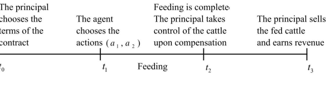
Consider a principal agent relationship in which a risk neutral cattle owner (the principal hereafter) who owns feeder cattle and makes contractual arrangements with a risk averse feedlot operator (the agent hereafter) to feed the cattle until they are ready for slaughter. After choosing a particular payment scheme from a menu of contracts, the principal delivers the cattle to the agent’s premise on an agreed date. The agent feeds the cattle high-energy rations until they are ready for slaughter. When the cattle gain desired weight, the principal makes payment to the agent for feeding the cattle according the contract and earns revenue by selling the fed cattle to a beef packer. The sequence of actions of the principal and the agent is outlined in figure 1.

The principal

chooses the The agent

terms of the chooses the the fed cattle

contract actions and earns revenue

Feeding is completed

The principal sells

Feeding

Figure 1. Sequence of Actions The principal takes control of the cattle upon compensation 0 t t₁ t₂ t₃ ) , (a1 a2

Assume that the entire process has four time periods. At period , the principal chooses a payment scheme from the menu of cattle feeding contracts and offers it to the

0 t

agent. Attention is limited to only linear contracts with fixed fee and incentives based on the full vector of contractible variables.7 If the agent accepts the terms of the contract, the principal delivers the cattle to the feedlot at period . The agent then starts feeding the cattle by choosing a two-element vector of actions

1 t ) , (a₁ a₂ a = at cost per

hundred pounds of live weight gain. The feedlot operator’s actions and primarily affect yield and quality of the beef procured from each hundred pounds of live weight. Assuming a linear functional form, the relationship between agent’s actions and actual yield and quality of beef can be written as:

) , (a₁ a₂ c 1 a a₂ y q 2 12 1 11 0 0 y y m a m a y y = +Δ = + + 2 22 1 21 0 0 q q m a m a q q= +Δ = + + a M l l = ₀ + (1)

where l is a vector of actual yield and quality of beef in each hundred pounds of live weight, is a vector of and which are threshold levels of yield and quality which are not affected by the feedlot operator’s actions, and

0

l y₀ q₀

y

Δ and Δqare incremental yield

and quality of beef which exclusively depend on the actions of the cattle feeder’s action during the feeding phase.8 Parameters m_ij with i, j∈{1,2} in matrix M represent

coefficients of production corresponding to the actions of the feedlot operator.

The linear production functions represented by equations in (1) nests two standard cases. First, one dimensional efforts (m₁₂ =m₂₂ =0), where attempts to improve yield

7 _{A theoretical justification for the use of linear contracts could be found in Holmstrom and Milgrom}

(1987) and Bhattacharyya and Laffontain (1995).

8 _{Assuming that the production functions are additively linear, it allows us to separately consider the effects}

also increases the quality of beef. Second, unproductive multitasking ( ), where attempt to increase yield is costly but does not affect the quality of beef, and vice versa. The agent’s actions and are assumed to be yield and quality improving, respectively, such that the elements with

0 21 12 =m = m 1 a a₂ ii

m i∈{1,2}are positive. The off-diagonal

element mij with i≠ j of the coefficient matrix,M , is a measure of systematic

complementarity (or substitutability in case the sign is negative) between the actions in the production function. For analytical simplicity, I assume that M is symmetric and

positive definite.

The cost function is assumed to be twice continuously differentiable, strictly increasing, strictly convex in both of its arguments, and is represented by a quadratic function of the form

) , (a₁ a₂ c

[

]

where, the off-diagonal element c_ij with i≠ j in the symmetric matrix Cis a measure of the degree of effort substitutability (or complementarity in case the sign is negative).

At period , the cattle reaches desired weight and the principal resumes the control of the fed cattle upon making payment to the agent for cattle feeding according to the linear incentive contract chosen at period . The actions of the cattle feeder during the feeding phase are not directly observable or verifiable by the principal. Neither does she observes the final yield and quality of beef upon delivery of the fed cattle. However, the owner observes the additional weight gained by the cattle during the feeding period and the number of days the cattle were on feed. Based on these information and also on

2 t

0 t

some other objective or subjective measures, the principal makes an assessment of potential yield and quality of beef. It should be noted that while there is an objective measure of potential yield, the measurement of beef quality is very subjective.

Let the measures of incremental yield and quality be linear functions of the agent’s actions and are given by

1 2 12 1 11 0 1 2 1, ) ( +ε = + + +ε = f a a y m a m a s_y 2 2 22 1 21 0 2 2 1, ) ( +ε = + + +ε = g a a q m a m a s_q (3) ⎥ ⎦ ⎤ ⎢ ⎣ ⎡ = Σ Σ + + = ⎥ ⎦ ⎤ ⎢ ⎣ ⎡ = 2 2 12 12 11 0 , ~ (0, ), _{σ σ} σ σ ε ε N Ma l s s S q y

where is a vector of measured yield and quality and respectively) of beef obtained from hundred pounds of live weight, and

S (sy sq

ε is a vector of random variables that have a bivariate normal distribution. The variance σ_ii of the random variable ε_i is a measure of both the difficulty that the agent has in controlling yield and quality of beef and the difficulty that the principal has in measuring the output, or in observing the actions of the agent. The covariance between the εi and εj, σij is a measure of random

complementarity (or substitutability) between the actions of the agent.

According to the linear compensation scheme, the agent receives a fixed fee per hundred pounds of live weight gain, α, (that covers feed cost and yardage charges for each hundred pound of live weight gain), and incentives, β₁ and β₂, for incremental yield and quality per hundred pounds of added weight. Thus the agent’s net income per hundred pounds of live weight gain,x, is

[

]

Feed cost plus yardage fee and flat-rate-per-pound-of-gain are two special cases of the linear payment scheme in equation (4). Equation (4) represents feed cost plus yardage fee contract whenβ₁ =0 and β₂= 0, and flat-rate-per-pound-of-gain contract when α =0 and β₂ = 0.

Let the agent’s total income from cattle feeding is given by X =kx, where is the number of hundred pounds of meat (the scale of operation) the feedlot is able to produce in the short run. Denoting the agent’s constant absolute risk aversion (CARA) coefficient by

k

φ and constant relative risk aversion coefficient by ψ , the risk preference of the agent can be represented by a negative exponential utility function of the form

) exp( )

(X x

U =− −ψ , where ψ =E(ψ /x)=ψ /x =φk.9 Thus, the agent’s certainty

equivalent income per hundred pound of weight gain is given by

β β ψ β α + + − − Σ = T T T a Ca a M l ACE 2 2 ] [ ₀ (5)

The last term in equation (5) is the variance of the agent’s income under the linear compensation scheme. Thus, the feedlot owner’s certainty equivalent income is his expected compensation from the linear payment scheme, minus the private cost of the agent’s actions, minus a risk premium.

Finally, at period , the principal sells fed cattle to a packer and realizes revenue. The principal can sell the fed cattle either through open outcry livestock actions on a live weight basis where the packers are bidders, or sell them to an individual packer using a dressed weight or a grid pricing method through some kind of marketing agreement. Live

3 t

9 _{This framework takes account of the effect of the scale of operation on the agent’s risk preference. In}

particular, it implies that the agent follow CARA in the short run but adapt to CRRA over the longer run as scale (k)changes.

weight pricing of fed cattle can be regarded as an outside option for the producer, as this is still the predominant method of marketing fed cattle. In any case, packers value both the quality and quantity of beef procured from the animals, which in turn depend on the actions taken by agent during the feeding phase.

When the fed cattle are priced on a grid, the packer pays a base price for the benchmark yield and quality combination, plus premiums (or discounts) for actual incremental yield and quality. Let B denote the base payment for yield and quality

combination and per hundred pounds of live weight, be the price premium for the incremental yield , and be the premium for the incremental quality . Thus, when the cattle are priced on a grid, the principal’s income per hundred pounds live weight is 0 y q₀ p₁ y Δ p2 Δq

[

]

The grid price mechanism above nests the other two pricing methods. When there is no premium for beef quality (i.e., when p₂ =0) it represents dressed weight pricing, and when there is no premium at all (i.e., p₁ =0 and p₂ =0) it represents live weight price. Assuming that the principal is risk neutral, her certainty equivalent net income is her expected revenue minus expected payment to the agent under a linear compensation scheme. (6) ] [l₀ M a a M p B S a M p B PCE = + T −α − βT = + T −α − βT +

The efficient incentive contracts are those that maximize the joint surplus of the principal and the agent subject to the agent’s incentive constraint. The joint surplus is the

total certainty equivalent of the principal and the agent under grid pricing of fed cattle and the linear compensation rule for cattle feeding

2 2 β β ψ Σ − − + = + = T aTCa T a M p B PCE ACE TCE . (7)

The expression in equation (7) is independent of the intercept term α. The principal chooses a and β to maximize the total certainty equivalent, and then uses α to transfer some of the surplus to the agent in an unspecified fashion. The principal’s problem is therefore to 2 2 , β β ψ β Σ − − + T T T a a C a a M p B Maximize

subject to the agent’s incentive constraint

⎥ ⎦ ⎤ ⎢ ⎣ ⎡ − + + ∈ 2 ] [ max arg k₀ Ma a Ca a T T β α

The incentive constraint states that, for any given β, the agent chooses the level of and that maximizes his expected net income. From the first order condition of the agent’s maximization problem we have

1 a a₂ β M C a∗ = −1 (8)

Differentiating (8) with respect toβ, when is strictly positive in all components, we obtain a 2 12 22 11 12 12 11 22 1 1 c c c m c m c a − − = ∂ ∂ β 2 12 22 11 22 12 12 22 2 1 c c c m c m c a − − = ∂ ∂ β 2 12 22 11 11 12 12 11 1 2 c c c m c m c a − − = ∂ ∂ β 2 12 22 11 12 12 22 11 2 2 c c c m c m c a − − = ∂ ∂ β .

Given that (m₁₁,m₂₂,c₁₁, andc₂₂ >0), the sign of ∂a_i /∂β_i for i∈{1,2}is non-negative

and the sign of ∂a_i/∂β_j for i≠ j is non-positive if m₁₂ ≤ 0 and (the signs are strictly positive and strictly negative for strict inequality in the sufficient conditions). In other words, when the actions are substitutes in the production function (i.e., ) and also in the agent’s cost function (i.e., ), the agent chooses an action ,

, that increases with

0 12 ≥ c 0 12 ≤ m 0 12 ≥ c a_i } 2 , 1 { ∈

i βi and decreases with βj, i ≠ j. Similarly, the signs of

i i

a ∂β

∂ / for i∈{1,2} and ∂ai/∂βj for i ≠ j are non-negative (positive with strict

inequality in the sufficient conditions) if the actions are complements in the production and cost function (i.e., if m₁₂ ≥0, and c₁₂ ≤ 0).

Substituting equation (8) into the objective function, the principal’s problem can therefore be written as 2 2 1 1 _β β β ψβ β β Σ − − + T − TMC− M T M MC p B Maximize .

Assuming that a∗ >0, the optimal value of β can be computed from first order necessary conditions for this unconstrained maximization problem as

[

]

∗ _{= +ψ Σ}

β (9)

where is the optimal incentive contract. It is useful to examine special cases in order to understand the implications of the structure of the optimal contract in (9).

∗

β

No uncertainty or risk neutrality

In the case of certainty (Σ=0) or if the agent is also risk neutral ( ) like the principal, (9) reduces to

0 = r

p = ∗

β . (10)

This implies that the principal transfers the yield and quality premiums earned in the grid directly to the agent. If the fed cattle are sold according to dressed weight, the principal transfers only the yield premium, as under the dressed weight pricing method

0 2 2= p =

β . Under the live weight pricing methodp₁= p₂= 0, which implies that 0

2 1 = β =

β . However, the principal can extract a part (or the whole) of the transferred premiums (in the case fed cattle are priced in a grid or according to dressed weight) from the agent through the use of α. Thus, the special case with no uncertainty or risk

neutrality is a standard transfer pricing problem.

The agent’s activities are unrelated (no multitasking)

When the agent’s actions are systematically and stochastically unrelated (i.e., 0

12 12

12 =c =σ =

m ), it is straightforward to show that

ii i ii i ii i c r m p m 2 2 2 σ β + = ∗ (11)

Thus, when the agent’s activities are unrelated, the optimal incentive for the th task is independent of the characteristics of the

i

jth activity. Moreover, the principal offers a higher powered incentive to the agent when the premium goes up (i.e., is larger), and when the production function is more elastic with respect to the agent’s action

( 0

i

p

/∂ >

∂βi mii ). On the other hand, the principal gives lower powered incentives for a

higher (i.e., σii is larger), and when the cost function is more convex (?) (i.e., is

larger).

ii

c

The agent’s activities may not be independent and the signal for beef quality is

unobservable to the principal before slaughter

This case is tailored to fit the aspects of commercial cattle feeding and fed cattle pricing methods. In reality, the agent’s actions to improve yield and quality of beef are not independent ( ). For example, while use of growth promoting implants increases yield, the rate of weight gain, and feed efficiency, it also has potential negative effects on beef quality (Field and Taylor, 2002; Duckett, et al., 1996). On the other hand, a common practice to increase beef quality is to feed high grain rations during the

finishing phase, which increases the percentage of fat in the carcass. As a result, marbling (intramuscular fat), and hence beef quality increases, but at the cost of yield (Fox and Black, 1992). This tradeoff is particularly important when the fed cattle are priced on a grid according to actual yield and quality of beef. Another important issue for the

principal is that actual quality of beef is almost unobservable and immeasurable until the cattle are slaughtered. Therefore, in reality, we do not observe any cattle feeding

contracts offering incentive for beef quality ( 0 , 0 ₁₂ 12 ≠ c ≠ m 0 2 = β ).

In the case where the agent performs multiple tasks (m₁₂ ≠ 0,c₁₂ ≠0), and the quality of beef is immeasurable upon delivery of the fed cattle (or the signal of beef quality, , is unobservable to the principal), such that sq is infinite and

2 2

σ σ₁₂ is zero, the

optimal incentive for yield improving activity is given by (for formal derivation, please, see the Appendix)

) ( 2 )] ( ) ( [ )] ( ) ( [ 2 12 22 11 2 1 12 11 12 2 12 11 2 11 22 2 12 11 11 12 22 12 12 11 22 12 1 12 11 11 12 12 12 12 11 22 11 1 c c c m m c m c m c p m c m c m m c m c m p m c m c m m c m c m − + − + − − − + − − − = ∗ σ ψ β . (12) The main comparative statistic result that follows (12) is that, when the agent’s activities are substitute in the production and cost functions (i.e., when and

), a higher premium for actual yield leads to a higher powered incentive, and a higher premium for quality leads to a lower powered incentive (i.e., , and

). It follows that, for all other things equal, reaches its highest value when there is no premium for quality at all (

0 12< m 0 12 > c 0 / ₁ 1 ∂ > ∂ ∗ p β 0 / 2 1 ∂ < ∂ ∗ p β ∗ 1 β 0 2=

p ), as is the case in dressed weight pricing method. This implies that if the principal is predetermined to sell the fed cattle on a dressed weight basis, she will offer high powered incentive for yield improving activity. Thus, flat rate per pound of gain contract (highest powered incentive contract) for cattle feeding is more likely in the case the principal decided to price the fed cattle according to dressed weight.

Under a grid pricing mechanism, actual yield and quality of beef are measured after slaughter and both are rewarded accordingly. Therefore, the incentive for yield improving activity is likely to be lower as long as the beef quality premium is positive ( ) under the grid pricing of fed cattle. This result is consistent with the argument of Holmstrom and Milgrom that, when inputs are substitutes and one of the activities cannot be measured, then the only way to provide the incentive for that immeasurable activity is to reduce the incentive for the other (measurable or observable) activity.

0 2> p

Since the first term in (12) is positive and the second term is negative, it may be optimal for the principal to set β₁ equal to zero (negative) provided the two terms in the

numerator offset each other (the second term is greater than the first one in absolute value). Zero incentives can also arise in a limiting case when agents activities are perfect substitutes in the production function such that m₁₁ =m₁₂ =m₂₂ and yield and quality premiums are equal (p₁= p₂). In that case, both β₂ =0 and β₁ =0. This result explains why a majority of cattle are fed on the basis of a fixed fee (feed cost plus yardage

charges) per animal head per day.

The second comparative statistic result is that the effect of the degree of

substitutability of the agent’s actions in the production and cost functions (i.e., the effects of and ) on the optimal incentive contract is ambiguous in general. However, it can be shown that, for and ,

12 m c₁₂ 0 12< m c₁₂ > 0 0 ) ( 12 1 > ∗ < ∂ ∂ m β if ( 2) 12 22 11 2 1 2 11 22 ) ( 2 12 11m c m c c c c > + − < ψσ . (13)

In other words, the effect of substitutability in the production function can be determined under certain conditions. Finally, as in the case of unrelated efforts a lower powered incentive is associated with higher degree of risk aversion (larger r) and increased

uncertainty (larger σii).

4. Evaluation of the Theoretical Predictions by Simulation Experiment

Empirical evaluation of the comparative static results require ranch to rail data on cattle fed under various contract arrangements along with actual costs and revenues. Such data, however, are proprietary in nature and therefore not available publicly. Therefore, a simulation model is developed and employed to evaluate the theoretical predictions. The basic idea of the simulation model is to generate and compare net returns to the feeder

and the owner under various fed cattle pricing methods, contract types, and production technologies. Net returns to the feeder and the owner under alternative production and marketing practices are compared to determine the optimal technology and optimal contracts under each pricing methods. The first step in the comparative return simulation model is to define the structural profit functions and preferences of the cattle feeder and the owner under alternative payment systems and fed cattle pricing methods. Given

Profit and utility functions of the cattle feeder and the owner

Suppose, a cow-calf producer delivers weaned calves to a commercial feedlot operator for intensive feeding of the animals until they gain market weight. As described earlier, under the yardage fee contract, the owner pays to the feeder a fixed fee per animal head per day and bears all the variable cost of feeding. On the other hand, under the cost of gain contract, the feeder receives a piece rate per pound of weight gain and bears the total feeding cost. In either case, the cattle feeder’s profit can be calculated easily by subtracting the feeder’s share of the feeding cost from the contractual payment received from the owner of the animal. The cattle feeder’s partial profit from feeding each individual cattle can be described by the following equation that nests the profits under alternative payment schemes.

k , for ; subject to, if i f R i i i F

i =[α+β×ADG +(γ −1)×ADG ×FE ×P −C ]×DOF

π i=1,...k 0 = α , then γ =0, if β =0, then 1≤γ , and α α≤ ≤ 0 , 0≤β ≤β , and 0≤γ ≤γ . (14)

Where π_iFrepresents the feeder’s profit from feeding cattle i, α is the yardage charge

per animal head per day, β is the piece rate per pound of gain, γ is the feeder’s share of the variable cost of feeding, denotes price per pound of feed ration, represents

fixed cost per animal head per day, and , , and denotes average daily gain, feed efficiency, and days on feed of the animal, respectively. When

R P C_f i ADG FE_i DOF_i 0 = α

andγ =0, equation (14) represents the feedlot operator’s profit from feeding cattle i

under the cost of gain contract. Alternatively, when β =0 and 1≤γ , it represents the feeder’s profit under the yardage fee contract.

The feeder’s profit from feeding cattle is the sum of over all . Thus, the feeder’s average profit per head can be represented by

k πiF i's ⎟ ⎠ ⎞ ⎜ ⎝ ⎛ =

∑

Total shrunk weight gain by an animal can be expressed as a product of average daily gain and the number of days on feed. Therefore, the feeder’s average profit per hundred pounds of weight gain can be given by

⎟ ⎠ ⎞ ⎜ ⎝ ⎛ × × × =

∑

∑

The cattle owner takes the possession of the fed cattle upon paying the feeder according to the contract and sells the cattle either in the live, dressed, or grid market. As mentioned earlier, the grid pricing mechanism offers premiums and discounts for

incremental yield and quality of the beef procured from each individual animal. Under the dressed weight pricing method carcasses are priced according to the actual yield or

dressing percentage, thus paying a premium (discount) for higher (lower) yield on an average. However, the base prices in the dressed weight and grid pricing methods are typically established with historical cash live weight prices and expected dressing percentage. Yield premium is just the difference between the actual and expected dressing percentages multiplied by the base price. Therefore, the cattle owner’s profit from a grid that uses cash live weight prices for establishing the base price can be expressed by the following equation.

[

]

[

]

subject to, if α =0, then γ =0, if β =0, then 1≤γ , and

α α≤ ≤

0 , 0≤β ≤β , and 0≤γ ≤γ , (17) where stands for initial shrunk body weight of the feeder cattle, and denote prices of fed and feeder cattle per hundred pounds of live weight, and are actual and expected dressing percentages,

ISBW P_L P_F

A

DP DP_E

Y

ρ and ρ_Q represent yield and quality grade

premiums, and and are incremental yield and quality grades, respectively. Equation (17) also nests the owner’s profits from live and dressed weight pricing of the cattle. In particular, when there are no yield and quality grade premiums (i.e.,

Y Δ ΔQ 0 = Y ρ and ) 0 = Q

ρ , then equation (17) represents the owner’s profit from dressed weight pricing.

under live weight pricing. The cattle owner’s average profit per head and per hundred pounds of weight gain are given by

⎟ ⎠ ⎞ ⎜ ⎝ ⎛ =

∑

∑

∑

Following the convention of the expected utility theory, preferences of the risk averse cattle feeder and the owner can be represented by expected utility functions. Let

and denote the total net profits of the feeder and the owner, respectively. Assuming constant absolute risk aversion from both of the feeder and the owner’s part, their utilities from the operation are given by

F Π _ΠO ) ; (20) exp( F F U =− −ϕΠ ) ; (21) exp( O O U =− −φΠ

where ϕ and φ are CARA coefficients of the feeder and the owner, respectively. The assumption of constant absolute risk aversion implies that relative risk aversion is increasing in scale. Arrow (1970) ahs made convincing arguments against the possibility of increasing relative risk aversion. The effect of scale of operation on the agents’ risk preference can be incorporated with an approximation of the constant relative risk aversion (CRRA) coefficients.

Assume that the feedlot has the capacity of feeding Kcattle simultaneously, and

the full capacity of the feedlot is utilized by feeding cattle heads from identical feeder cattle owners. Thus, total net profit of the feeder is given by

k n F F F nk Kπ = π = Π .

F

nkπ

ϕ

ψ = , the feeder’s utility from feeding k cattle of a single owner can be expressed as ) ˆ exp( F F U =− −ψπ , (22)

where ψˆ =E(ψ /nπF)=ψ /nπˆF =ϕk. In a similar fashion, the cattle owner’s CRRA

preference can be represented as ) ˆ exp( O O

U =− −θπ , (23)

where θ denotes the owner’s CRRA coefficients, and θˆ= E(θ /πF)=θ/πˆO =φk.

Thus, both the feeder and the owner follow CARA in the short run but adapt to CRRA in the longer run (as scale of operation changes).

Simulation procedures

Given the cattle performance data and price information, net returns to the feeder and the cattle owner can be calculated according to the profit functions as defined above. In the absence of actual feedlot and carcass data, a dynamic and deterministic

bio-physical growth model for beef cattle is adapted that is able to systematically predict daily feed intake, weight gain, and composition of the gain by each individual animal given feeder cattle’s genetic and biological information, net energy and protein values of the ration, and weather condition. A data set containing cow-calf information and partial feedlot and carcass performances of 1131 steers are obtained from Tri-county Steer Carcass Futurity (TCSCF) program. Growth performances of these steers under eighteen ration-implant strategies are simulated using the bio-physical model. Six alternative rations with known energy and protein values along with three implant strategies are employed. Since the steers were placed in the feedlots of southwester Iowa during

October-December of 1995-98 and harvested during April-June of the following year, a typical Fall-Spring weather condition of southwestern Iowa is assumed. Initial and final body weights of the cattle, total dry matter intake and weight gain during the feedlot regime, final carcass weight and yield and quality grades of the carcasses are retained to use in the comparative returns model. A detailed description of the growth model and an analysis of the simulated outcomes are available in the Appendix.

Combining the cattle performance data generated by the growth model with historical price data, stochastic returns under various fed cattle pricing methods, contract types, and production technologies are computed. Historical weekly average prices for fed cattle, feeder cattle, feed ingredients, and grid premiums and discounts data are obtained from the United States Department of Agriculture (USDA). Weekly weighted average live and dressed weight prices for fed cattle, live weight prices for feeder cattle, and weekly average prices for corn during January 1996 through December 1999 in Iowa are obtained from the Agricultural Marketing Services (AMS) of the USDA. Corn silage prices are calculated using corn prices assuming 34 percent dry matter content. Iowa prices for soybean meal and alfalfa hay were not available through the USDA. Therefore, weekly average prices for soybean meal in Decatur, Central Illinois, and weekly average prices for alfalfa hay in Kansas are obtained for the same period. Weekly average yield and quality grade premiums and discounts paid in the grid under voluntary price reporting during 1996-99 and under mandatory price reporting during 1999-current are also collected. Weekly average grid premiums and discounts reported under mandatory price reporting provision of the USDA during 2002-05 are used instead of the voluntarily reported ones.

Following historical profitability reports of several Iowa feedlots, yardage fee and other fixed cost per cattle head per day are determined. During the period of 1996-99, average yardage fee charged by the feedlots per cattle head per day was around 25 cents. Labor, utility, and interest on feed are found to be 20 cents per cattle head per day. Some feedlots which feed cattle under the cost of gain contracts reported that the average charge per pound of gain to be around 45 cents. Using average daily gain and feed efficiency reported by TCSCF and historical feed cost data, equivalent cost of gain payments equivalent to the yardage fee payments of 20-35 cents are imputed with the increment of one cent. The cost of gain payment equivalent to 20 and 35 cents of yardage charge were found to be 43.3 and 48.1 cents, respectively, and each incremental cent in the yardage fee resulted into a 0.3 cent increment in the cost of gain payment. Therefore, 25 and 44.9 cents are used in the simulation as the benchmark yardage fee and cost of gain payments, respectively.

Stochastic costs and returns of the feeder and the owner are calculated in a Monte Carlo fashion using the historical weekly average prices and the feedlot budget. Since cattle and feed ingredient prices are likely to be correlated, the prices are drawn from the multivariate distribution of the data after estimating their multivariate kernel densities.10 Using a multivariate random draw, feeding costs under each production situation and returns from selling the fed cattle through live weight, dressed, weight and grid pricing are calculated. Net profits of the feeder and the cattle owner are then calculated according to the profit functions as described above. The procedure is iterated for 5,000 times for each individual cattle and production technologies. Finally, average net returns (over the

10 _{Using the entire sample, Kolmogorov-Smirnov (K-S) tests were performed on each series. The}

iterations) per head and per hundred pounds of weight gain to the feeder and the owner are calculated.

Simulation results

Following the procedures as described above, two separate simulation

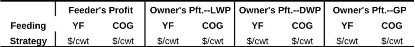
experiments are carried out. In the first experiment, net returns are calculated assuming that the cattle are fed until they reach a target body weight. In the second experiment, net returns are calculated holding the number of days on feed fixed. Assuming that the agents decisions were optimal, final shrunk body weights and days on feed reported in the TCSCF data are used as the terminal conditions in the simulations experiments. Resulting expected profits to the feeder and the owner per hundred pounds of added weight under alternative production technology, cattle feeding contracts, and fed cattle pricing methods are presented in Tables 1 and 2. Table 1 shows the results of the simulation experiment 1 (with fixed terminal state), while Table 2 displays the result of the simulation experiment 2 (with fixed terminal time).

The feeder’s expected profits per hundred pound of added weight from the alternative feeding strategies under the two types of contracts are listed in columns two and three of the tables. Results of the both simulation experiments show that the feeder’s profit under the yardage fee contract decreases with the grain-silage ratio of the ration and the potency of the growth promoting implants. This is because days on feed (total shrunk weight gain) decreases (increases) with the percentage of grain in the ration and the productivity of the implants with fixed terminal state (with fixed terminal time). On the other hand, under the cost of gain contract, the feeder’s profit increases with the

productivity of the implants, and decreases with the percentage of grain in the feed with no implant but increases with the ratio of grain in the feed with implants. This is mainly because the substitutability between the energy content of the ration and the productivity of implants (see Appendix Tables 5 and 6).11 The pattern of changes in the expected profits of the cattle owner under alternative contracts can be explained with the same arguments.

11 _{The rate of decrease in required days to reach a target body weight for higher energy content of the ration}

Table 1: The feeder and the cattle owner's expected profits under alternative production technologies, feeding contracts, and fed cattle pricing methods (Results from simulation experiment 1 - fixed terminal state)

Feeding YF COG YF COG YF COG YF COG

Strategy $/cwt $/cwt $/cwt $/cwt $/cwt $/cwt $/cwt $/cwt No Implant Ration 1 11.88 -3.30 -2.76 12.43 -5.95 9.23 -3.62 11.56 Ration 2 11.42 -2.89 -1.87 12.43 -5.07 9.23 -2.42 11.89 Ration 3 11.03 -2.60 -1.21 12.43 -4.40 9.23 -1.44 12.19 Ration 4 10.68 -2.36 -0.61 12.43 -3.81 9.23 -0.62 12.42 Ration 5 10.38 -2.18 -0.13 12.43 -3.32 9.23 0.03 12.58 Ration 6 10.10 -2.04 0.29 12.43 -2.91 9.23 0.60 12.74 Estrogen only Ration 1 9.38 3.73 6.78 12.43 3.58 9.24 1.50 7.15 Ration 2 9.07 3.80 7.16 12.43 3.97 9.24 2.15 7.42 Ration 3 8.79 3.88 7.51 12.43 4.32 9.24 2.78 7.70 Ration 4 8.55 3.91 7.79 12.43 4.60 9.24 3.23 7.87 Ration 5 8.33 3.95 8.05 12.43 4.86 9.24 3.71 8.09 Ration 6 8.13 3.95 8.25 12.43 5.06 9.24 4.11 8.29

Estrogen plus TBA

Ration 1 8.28 6.54 10.69 12.43 7.50 9.24 0.71 2.45 Ration 2 8.00 6.59 11.02 12.43 7.83 9.24 1.28 2.70 Ration 3 7.76 6.65 11.33 12.43 8.14 9.24 1.84 2.94 Ration 4 7.54 6.68 11.57 12.43 8.38 9.25 2.32 3.19 Ration 5 7.34 6.71 11.80 12.44 8.62 9.25 2.78 3.41 Ration 6 7.17 6.71 11.98 12.44 8.79 9.25 3.12 3.57

Table 2: The feeder and the cattle owner's expected profits under alternative production technologies, feeding contracts, and fed cattle pricing methods (Results from simulation experiment 2 - fixed terminal time)

Feeding

Strategy YF COG YF COG YF COG YF COG

$/cwt. gain$/cwt. gain$/cwt. gain$/cwt. gain$/cwt. gain$/cwt. gain$/cwt. gain$/cwt. gain

No Implant Ration 1 11.73 0.66 -1.49 9.59 -6.58 4.49 -20.34 -9.27 Ration 2 11.31 0.66 -0.70 9.94 -5.51 5.14 -18.01 -7.37 Ration 3 10.94 0.65 -0.04 10.26 -4.59 5.71 -15.59 -5.29 Ration 4 10.62 0.56 0.47 10.53 -3.86 6.20 -13.45 -3.39 Ration 5 10.34 0.48 0.90 10.77 -3.23 6.63 -11.47 -1.61 Ration 6 10.10 0.34 1.22 10.98 -2.74 7.01 -9.54 0.21 Estrogen only Ration 1 9.77 4.46 5.93 11.24 2.19 7.50 -8.19 -2.89 Ration 2 9.43 4.36 6.45 11.52 2.95 8.02 -5.83 -0.76 Ration 3 9.14 4.25 6.89 11.77 3.58 8.47 -3.65 1.24 Ration 4 8.88 4.09 7.20 11.99 4.08 8.87 -1.45 3.34 Ration 5 8.66 3.94 7.46 12.18 4.50 9.22 0.31 5.03 Ration 6 8.46 3.74 7.64 12.35 4.81 9.52 2.04 6.75

Estrogen plus TBA

Ration 1 8.68 6.29 9.75 12.15 6.76 9.15 -2.66 -0.26 Ration 2 8.39 6.17 10.18 12.40 7.40 9.62 -0.46 1.76 Ration 3 8.13 6.04 10.54 12.62 7.93 10.02 1.76 3.84 Ration 4 7.90 5.86 10.78 12.82 8.34 10.37 3.64 5.67 Ration 5 7.70 5.70 10.99 12.99 8.68 10.68 5.38 7.37 Ration 6 7.52 5.50 11.11 13.14 8.93 10.95 7.14 9.17

Feeder's Profit Owner's Pft.-LWP Owner's Pft.-DWP Owner's Pft.-GP

The cattle owner’s expected profit maximizing feeding contract types under the live weight, dressed weight, and grid pricing methods, and the feeder’s expected profit maximizing choice of the production technology under the yardage fee and cost of gain contracts can be easily determined from the tables. It should be mentioned here that under the yardage fee contract the cattle owner has the right to choose the technology as he pays for the feeding costs (feed and implant costs). The feeder bears only the fixed costs of

feeding (labor and utilities) and provides the services in exchange for the fixed yardage fee per animal head per day. On the other hand, under the cost of gain contract, the feeder bears all the costs and receives a fixed payment per pound of added weight, and therefore chooses the production technology that maximizes his return. The cattle owner does not have any discretion in choosing the feeding strategy under the cost of gain contract.

Both of the simulation experiments show that from the owner’s perspective the cost of gain contract is optimal when cattle are to be priced according to the live weight and dressed weight pricing methods. And, as the owner chooses the cost of gain contract to feed the cattle, the feeder finds it optimal to use high-potency implants (estrogen plus trenbolon acetate) and relatively lower percentage of grain in the feed. On the other hand, the yardage fee contract is optimal for the cattle owner when the fed cattle are to be priced on the grid. It also shows that a production technology with high energy feed and a moderate implant strategy is optimal for the owner as the cost savings from the use of the high-potency implant (estrogen plus Trenbolon Acetate) is not enough to cover the loss of revenue due to the sacrificed beef quality.

Thus, the comparative return simulation confirms the prediction of the multitask model presented in section three of this paper. In particular, the simulation experiments also confirm that when the feeder’s actions that affect beef yield and quality are

substitutes but the action that alters beef quality is not measurable then a lower powered incentive for the yield improving activity is optimal for the cattle owner if the fed cattle are priced according to actual yield and quality. However, if the cattle are to be priced according to a method that rewards higher yield only, then a higher powered incentive contract (e.g., cost of gain) is optimal.

5. Summary and Conclusion

This paper evaluates the optimal incentive structure in the existing cattle feeding contracts under alternative fed cattle pricing methods. In particular, incentive provisions in the yardage fee and cost gain contracts for cattle feeding are theoretically analyzed and evaluated considering the live weight, dressed weight, and grid pricing methods for fed cattle marketing. Following the seminal work of Holmstrom and Milgrom (1991), a multitask principal agent model is developed that captures the organizational details of beef cattle production and marketing. In the absence of a complete ranch to rail data, the comparative statics from the theoretical model are evaluated with simulation

experiments. Feedlot and carcass performance of a large set of feeder steers are simulated employing a dynamic and deterministic bio-physical growth model adapted from the animal science literature. The cattle feeder and the owner’s stochastic costs and returns under alternative production technologies and market conditions are then calculated by combining cattle performance data with historical price data. The expected profit

maximizing actions of the cattle feeder under alternative compensation schemes, and the cattle owner’s optimal choice of the incentive schemes under alternative fed cattle pricing methods are then determined by comparing the stochastic returns.

The simulation results confirms the main comparative static result of the multitask model that, when the feeder’s activities are substitute in the production and cost functions and the action that alters beef quality is not measurable, a higher premium for actual yield leads to a higher powered incentive and a higher premium for quality leads to a lower powered incentive. In other words, the main finding of this study is that, from the cattle owner’s point of view, the yardage fee (zero incentive) contract is optimal when the fed

cattle are to be priced on the grid and the cost of gain contract (high powered incentive for yield) is optimal when the cattle are to be marketed according to the live or dressed weight pricing methods.

Although the finding of this research is interesting, further research is required to test the robustness of the result. Especially, risk preferences of the agents are yet to be incorporated in the simulation experiments and a complete menu of contract payments need to be evaluated. Moreover, since commercial cattle feeding is in practice in different regions of the U. S., it needs to be examined if weather pattern and crop production practices have any effect on the incentive provisions. The author intends to extend the research along this line in near future.

References

Albright, M. L., T. C. Schroeder, and M. R. Langemeire. 1994. “Determinants of cattle feeding cost-of-gain variability.: Journal of Production Agriculture, 7: 206-210. Fox, D. G., and T. P. Tylutki. 1998. “Accounting for the effects of environment on the

nutrient requirements of dairy cattle.” Journal of Dairy Science, 81: 3085-95. Fox, D. G. and J. R. Black. 1984. “A system for predicting body composition and

performance of growing cattle.” Journal of Animal Science, 58(3): 725-739. Fox, D. G., C. J. Sniffen, J. D. O’Connor, J. B. Russel, and P. J. Van Soest. 1992. “A net

carbohydrate and protein system for evaluating cattle diets: III. Cattle requirements and diet adequacy.” Journal of Animal Science, 70: 3578-96. Garrett, W.N. and N. Hinman. 1969. “Re-evaluation of the relationship between carcass

Guiroy , P. J., D. G. Fox, L. O.Tedeschi, M. J. Baker, and M. D. Cravey. 2001. “Predicting individual feed requirements of cattle fed in groups.” Journal of Animal Science, 79: 1983-95.

Holmstrom, B. and P. Milgrom. 1991. “Multitask principal-agent analyses: Incentive contracts, asset ownership, and job design.” Journal of Law, Economics, and Organization, 7(special issue): 24-52.

Langemeire, M. R., T. C. Schroeder, and J. Mintert. 1992. “Determininants of cattle finishing profitability.” Southern Journal of Agricultural Economics, 24: 41-47. Mark, D. R., T. C. Schroeder, and R. Jones. 2000. “Identifying economic risks in cattle feeding.” Journal of Agribusiness, 18(3): 331-344.

National Research Council. 2000. Nutrient Requirements of Beef Cattle. National Academy Press, Washington D.C.

Pery, T. C. and D. G. Fox. 1997. “Predicting carcass composition and individual feed requirement in live cattle widely varying in body size.” Journal of Animal Science, 75: 300-307.

Schroeder, T. C., M. L. Albright, M. R. Langemeire, and J. Mintert. 1993. “Factors affecting cattle feeding profitability.” Journal of the American Society of Farm Managers and Rural Appraisers, 57: 48-54.

Tedeschi, L. O., D. G. Fox, and P. J. Guiroy. 2004. “A decision support system to improve individual cattle management. 1. A mechanistic, dynamic model for animal growth.” Agricultural Systems, 79: 171-204.

Tedeschi, L. O., D. G. Fox, and M. J. Baker. 2003. “The Cornell value discovery system model.” Model Documentation. Department of Animal science, Cornell

University, Ithaca.

Trapp, J. N., and S. D. Cleveland. 1989. “An analysis of the sources of profit volatility in cattle feeding.” In Proceedings of the NCR-134 Conference on Applied

Commodity Price Analysis, Forecasting, and Market Risk Management. Held in Ames, IA, April 1989. Iowa State University press, Ames, IA: 161-176.

Weimer, M. R. and A. Hallam. 1990. “Risk sharing in custom cattle feeding.” North Central Journal of Agricultural Economics, 12(2): 279-291.

Appendix 1

The Bio-physical Growth Model for Beef Cattle

With significant advances in understanding complex biophysical relationships and rapid progress in computation technology in recent years, several mathematical models have been developed to simulate beef cattle production system. The major goal of such models has been either to predict animal performance given a fixed feed resource or to predict feed requirements that support a fixed level of production. Lofgreen and Garrett (1968) first published a simple growth simulation model based on the NE system to compute feed requirements when performance is fixed. Fox and Black (1977a-c, 1984) altered the Lofgreen and Garrett model to predict performance when voluntary feed intake and energy content of feeds are known. They also generalized the model to account for the differences in breed, mature size, growth promoting implants, and feed additives. Since the introduction of Fox and Black model, continuous evaluations and necessary modifications have been made to improve its accuracy under alternative management practices and production situations (Fox et al., 1988, 1992; Tylutki et al., 1994; Perry and Fox, 1995; Fox and Tylutki, 1998). Successive beef cattle nutrition subcommittees of the National Research Council (NRC, 1996, 2000) have fully adopted the revised model after further evaluation with experimental data. The latest version of the model is described and documented by Fox et al. (2003).

Using the procedures and equations as described in NRC (1996, 2000) and Fox et al. (2003), researchers in the department of Animal Science at Cornell University have developed a dynamic and mechanistic growth model with daily time step that can be applied in feedlots to predict growth rate, accumulated weight, days required to reach

target body composition, and carcass weight and composition of individual animal (Tedeschi et al., 2004). The dynamic model is able to predict either average daily gain (ADG) when daily dry matter intake (DMI) is known or dry matter required (DMR) when ADG is known (Tedeschi et al., 2004). When evaluated with a large data set obtained from individually fed steers, the model accounted for more than 80 percent of variation in predicting individual animal ADG or DMR (Tedeschi et al., 2004). The dynamic growth model is being applied in a computer program called Cornell Value Discovery System (CVDS) developed to predict performance and costs of feeding individual animals in group pens.

The CVDS model, however, is applicable only when either ADG or DMI is observed, while both of these variables remain unknown to the cattle feeder and/or the cattle owner before feeding the cattle. Another limitation of the CVDS model is that it is unable to simultaneously predict cattle performance under alternative feeding strategies. For the purpose of this study, an integrated bio-physical growth model is required that is capable of predicting daily voluntary DMI by each individual animal and resulting gain and its composition under alternative production technologies. Such a model is developed by adapting the CVDS model with the complements of several sub-models published in the NRC (1996, 2000) reports and other relevant animal science research. For a wide range of alternative feed-implant strategies, the model can predict dry matter intake by each individual animal on each day on feed, resulting daily weight gain and composition, final weight and yield and quality grades of the carcass, and days required to reach a target harvest body weight or final body weight and composition for a given feeding period.