Validation of aggregated risks models

Archive University of Zurich Main Library Strickhofstrasse 39 CH-8057 Zurich www.zora.uzh.ch Year: 2018

Validation of aggregated risks models

Dacorogna, Michel ; El Bathouri, Laila ; Kratz, Marie

Abstract: Validation of risk models is required by regulators and demanded by management and share-holders. Those models rely in practice heavily on Monte Carlo (MC) simulations. Given their complexity, the convergence of the MC algorithm is difficult to prove mathematically. To circumvent this problem and nevertheless explore the conditions of convergence, we suggest an analytical approach. Considering standard models, we compute, via mixing techniques, closed form formulas for risk measures as VaR or TVaR on a portfolio of risks, and consequently for the associated diversification benefit. The numerical convergence of MC simulations of those various quantities is then tested against their analytical evalua-tions. The speed of convergence appears to depend on the fatness of the tail of the marginal distributions; the higher the tail index, the faster the convergence. We also explore the behavior of the diversification benefit with various dependence structures and marginals (heavy and light tails). As expected, it varies heavily with the type of dependence between aggregated risks. The diversification benefit is also studied as a function of the risk measure, VaR or TVaR.

DOI: https://doi.org/10.1017/S1748499517000227

Posted at the Zurich Open Repository and Archive, University of Zurich ZORA URL: https://doi.org/10.5167/uzh-169851

Journal Article Published Version Originally published at:

Dacorogna, Michel; El Bathouri, Laila; Kratz, Marie (2018). Validation of aggregated risks models. Annals of Actuarial Science, 12(2):433-454.

First published online 4 December 2017

Validation of aggregated risks models

Michel Dacorogna

DEAR-Consulting, Scheuchzerstrasse 160, 8057 Zurich, Switzerland

Laila Elbahtouri

SCOR, 5 Avenue Kléber, 75795 Paris, France

Marie Kratz*

ESSEC Business School, CREAR Risk Research Center, Avenue Bernard Hirsch, BP50105, 95021 Cergy-Pontoise, France*

Abstract

Validation of risk models is required by regulators and demanded by management and shareholders. Those models rely in practice heavily on Monte Carlo (MC) simulations. Given their complexity, the convergence of the MC algorithm is difficult to prove mathematically. To circumvent this problem and nevertheless explore the conditions of convergence, we suggest an analytical approach. Con-sidering standard models, we compute, via mixing techniques, closed form formulas for risk mea-sures as Value-at-Risk (VaR) VaR or Tail Value-at-Risk (TVaR) TVaR on a portfolio of risks, and consequently for the associated diversification benefit. The numerical convergence of MC simula-tions of those various quantities is then tested against their analytical evaluasimula-tions. The speed of convergence appears to depend on the fatness of the tail of the marginal distributions; the higher the tail index, the faster the convergence. We also explore the behaviour of the diversification benefit with various dependence structures and marginals (heavy and light tails). As expected, it varies heavily with the type of dependence between aggregated risks. The diversification benefit is also studied as a function of the risk measure, VaR or TVaR.

Keywords

Diversification (benefit); Heavy tail; Mixing technique; Model validation; Monte-Carlo simulation

1. Introduction

Risk and capital considerations are becoming central to the risk management of (re)insurance. In particular, the advent of risk-based solvency regulation like Solvency 2 in the European Union or the Swiss Solvency Test is bringing along many new requirements that push the industry in this direction. For instance, Solvency 2 Directive requires from (re)insurance companies to assess the capital needed to ensure their solvency. It is defined as the Value-at-Risk (VaR) of the own funds (the aggregated asset and liability risks) at a 1-year horizon subject to a confidence level of 99.5% over a 1-year period. The validation of this assessment is also required by the Directive and necessary for management to use the models for strategic decisions. It is not straightforward to validate results computed at such high threshold. Therefore, it should be tackled indirectly with various techniques. *Correspondence to: ESSEC Business School, CREAR Risk Research Center, Avenue Bernard Hirsch, BP50105, 95021 Cergy-Pontoise, France. E-mail: [email protected]

This paper is a step in this direction, proposing ways to check both the convergence of Monte Carlo (MC) algorithm and the behaviour of diversification benefit.

Understanding the diversification benefit is essential to the business model of reinsurance companies. Diversification is at the heart of efficient risk management, capital optimisation and competitive pricing. Internal models are considered as the best solution to monitor the risk within the (re)insurer’s portfolio and to compute the Solvency Capital Requirements, provided that the models are approved by the regulators. However, the authorities demand a validation of the whole modelling process and in particular of the techniques used. This implies thorough mathematical and best practice justifications of the choice of each distribution, assumption, parameter estimation, risk aggregation technique and so on (see Dacorogna, 2017). Most models are based on MC simulations of a large number of dependent risks. The convergence of such models is hard to prove mathema-tically and their stability, as a function of the number of simulations, is difficult to assess. The analytical approach is a way to measure the performance of the MC method, and potentially to replace it in some cases. Here, we propose this approach to improve our understanding and test the validity of model results.

Using standard models of the literature, we provide explicit expressions for the probability density function (pdf) of aggregated dependent risks, allowing to compute analytically risk measures as VaR or Tail Value-at-Risk (TVaR), and consequently the diversification benefit. This can be considered as a step towards the development of methods for model validation. To achieve this, we use mixing techniques (see Marshall & Olkin, 1988; Oakes, 1989) over risk parameter values. It is a standard tool in credibility theory, but less explored for actuarial dependent risks modelling. Whereas it has been used in ruin theory (see Albrecheret al., 2011), we introduce it for risk measures and diversification benefit. We could have used an alternative technique that has been proposed in Constantinescuet al. (2011) and Hashorva & Ji (2014), where conditional models are seen as simple random scaling models. But our purpose here is to concentrate on the numerical analysis in order to test the performance of the MC method.

On the same line of research, we use explicit formulas for the diversification benefit to explore its behaviour as a function of the aggregation factor and the risk measures through models examples exhibiting dependence or independence, and light or heavy tailed marginals.

The paper is organised as follows. We describe in section 2 the framework of constructing Archimedean copulas using the mixing techniques, deriving analytical expressions for risk measures and diversifi -cation benefit for two combinations of dependence structure and marginal distributions (Pareto– Clayton and Weibull–Gumbel). Note that special efforts have been put in presenting in a consistent and clear way the mixing techniques approach. In section 3, the numerical convergence of MC simulations of risk measures and diversification benefit is tested against the analytical results for those two dependent models, Pareto–Clayton and Weibull–Gumbel. In section 4, we compare the behaviour of the diversification benefit of models, from independence to various dependence forms. We study it as a function of risk measures and aggregation factors. General conclusions follow in the last section 5.

2. Analytical Results Via the Mixing Techniques

A general method for constructing multivariate Archimedean copulas has been introduced by Oakes (1989) in the bivariate case and extended in the multivariate case by Marshall & Olkin (1988).

The idea behind this method is to use the mixing technique over a latent variable as a tool for dependence modelling. Introducing a latent variable to transform dependent variables into con-ditionally independent ones, allows to express the dependence between the variables as an Archi-medean survival copula with parameter the latent variable, and to obtain the marginal distributions depending on this parameter. Namely, we have

The Oakes–Marshall–Olkin Theorem1

LetΘ_{be a positive random variable (rv) with cumulative distribution function (cdf)FΘandXk,k}≥1, be rvs such that

P X1ð >x1; :::;Xn>xn j Θ=θÞ= Yn

k=1

H xð Þk θ (1)

Hbeing a positive function. The dependence model specified by (1) is a variant of the structure dependence generated by an Archimedean survival copula with generatorϕ=L 1

Θ , whereLΘdenotes

the Laplace transform ofFΘ:

P X1½ >x1; ¼;Xn>xnŠ=LΘ X n i=1 LΘ1 FiðxiÞ ! (2) where the marginal distributionsFiofXi,i=1,…,n, are defined by

FiðxÞ: =1 FiðxÞ=LΘð lnHðxÞÞ (3)

By means of this mixing technique, we can provide an explicit formula for the pdf of aggregated risks Xi,i=1,…,n, of a dependence model. Finding the appropriate choice of the functionHand the

mixing parameterΘ_{tofit the marginals and the dependence model is the key step to derive via the}

Oakes–Marshall–Olkin theorem an explicit formula for the pdf. With the explicit pdf fS_n of the aggregate risk Sn: =Pn

i=1Xi, denoted by fn when no possible

confusion, we can derive the formulas for the risk measures and the diversification benefit. Recall that the diversification performance of a portfolio Sn is measured on the gain of capital when

considering a portfolio instead of a sum of standalone risks. The capital is defined by the deviation to the expectation, and the diversification benefit (Bürgiet al., 2008) at a thresholdκ(0<_κ<1), by

DκðSnÞ=1 ρκðSnÞ EðSnÞ Pn i=1 ρκðXiÞ EðXiÞ ð Þ =1 ρκðSnÞ EðSnÞ Pn i=1 ρκðXiÞ EðSnÞ (4)

whereρκdenotes a risk measure at thresholdκ. This indicator helps determining the optimal

port-folio of the company since diversification reduces the risk and thus enhances the performance. By making sure that the diversification benefit is maximal, the company obtains the best performance for the lowest risk. However, it is important to note thatDκ(Sn) is not a universal measure and

depends on the number of risks undertaken and the chosen risk measure.

We will consider two examples of dependent models, presented in Marshall & Olkin (1988) (and, since, considered in various papers, as, e.g., in Albrecher et al., 2011), that are useful in the

1 _{Note that we choose to denote this result asthe Oakes–Marshall–Olkin Theorem. It has been introduced}

and developed by Oakes for the bivariate case (see Oakes, 1989) and generalised for anynby Marshall & Olkin (1988).

reinsurance context. Thefirst model is with Pareto marginals and a Clayton structure of dependence, which is standard in reinsurance context as it captures the dependence in the tail. The second one considers Weibull marginals and a Gumbel copula; it is an interesting alternative since it combines tail dependence with thin tail distributions. Note that further examples have been considered in a recent preprint (Sarabiaet al., 2017).

Throughout the paper, we will assume the same threshold κfor any quantity defined w.r.t. this threshold, hence we will omit it in the notation of those quantities.

2.1. Pareto marginals with Clayton survival copula

In this example, we consider a dependent modelX=(X1,…,Xn) with marginals Fi (i=1,…,n)

(α,β)-Pareto (also called Pareto Lomax) distributed withα>1,β>0, i.e. such that FiðxÞ: =1 FiðxÞ= 1+x

β

α

; 8x>0; i=1; ¼;n (5)

Ifβ=_{1, we simplify the notation writingα-Pareto.}

Recall that the quantileq1of orderκof a (α,β)-Pareto cdf is given by

q1=VaRðκÞ=β ð1 κÞ 1=α 1

(6) The dependence structure of the model is chosen as a survival copula Cθ of Clayton form with

parameterθ>_{0, defined on [0,1]}n_by Cθðu1; ;unÞ=_φ 1 θ X n i=1 φθðuiÞ ! = X n i=1 u θ i ðn 1Þ ! 1=θ

with its generatorφ(invariant to multiplication of the argument by a positive constant) given by

φθðtÞ=t

θ _{1; t}

2 ½0;1Š (7)

First we need to compute the pdf of the aggregate riskSn=Pn_i

=1Xito evaluate the risk measures

VaR and TVaR ofSn, then deduce the associated diversification benefit. Computing directly the pdf

ofSnassociated to our dependent model may be a difficult task, hence the choice of using the mixing

technique to work with conditional independence. Assumingθ=_{1/α to ease the computation, we} obtain the following result.

Proposition 2.1 Consider the dependent model X=_(X1,…, Xn) with marginals Fi (i=1,…, n)

(α,β)-Pareto distributed (defined in (5)),α>_1,β>_{0, and Clayton survival copula defined in (7) with} parameterθ=_1/α>_{0. Then the pdffnof the aggregate riskSn}= P

n

i=1

Xiis compound Gamma (orβof the second kind with parameters (n,α)) given, fors>_{0, by}

fnðsÞ= β α Bðα;nÞ´ sn 1 β+s ð Þα+n (8)

Bdenoting theβfunction.

The choice θ=_{1/α is a constraint of this model. However, it can be generalised to separate the} dependence from the tail index. This is the subject of a forthcoming paper.

Having an explicit formula (8) for the pdffnofSn, we can deduce its cdfFSn integratingfn, and any

risk measure based onFSn.

The value-at-risk ofnat thresholdκ, denotedqκ,norqn, is obtained via:

qn=VaR_κðS_nÞ=F_S

nðκÞ (9)

F_Sn denoting the inverse ofFSn. Note that using the relation between aβdistribution of second kind

and aβdistribution,qnmay also be expressed in terms of the quantile of theβdistribution with the

same parameters,B(n,α),

qn= VaRκðBðn;αÞÞ 1 VaRκðBðn;αÞÞ

The TVaR ofSnat thresholdκ, defined by

TVaRn=TVaR_κð ÞSn =E_½Sn jSn≥qn_Š

(FSnbeing continuous), can be computed explicitly in terms ofqn, as done in the proposition below.

For completeness, let us compute the TVaR at thresholdκfor a (α,β)-Pareto cdf, assumingα>₁ (for the existence of the TVaR) andβ>_{0. We obtain}

TVaR1 : =TVaR_κð ÞX = β α 1 κ ð Þðα 1Þ´ αq1+β q1+β ð Þα; whereq1is given inð6Þ; i:e: TVaR1=β 1 1 1=α ð Þð1 κÞ1=α 1 (10)

Theorem 2.1 Considering the dependent Pareto–Clayton model X given in Proposition 2.1, the TVaR of the aggregate riskSn=Pn

i=1Xiat a thresholdκ, 0<κ<1, is given by TVaRn= β 1 κ ð ÞBðα;nÞB 1+ qn β 1 ;α 1;n+1 ! (11) whereB(x;a,b) denotes the incompleteβfunction defined by

B x_ð ;a;b_Þ= ðx

0

ua 1 _{1 u}

ð Þb 1du

If the shape parameterαof the Pareto margin is such thatα2Nn f0;1g, thenTVaRnsimplifies to

TVaRn = nβ ð1 κ_Þðα 1Þ 1 P α 2 j=0 n+_α 1 j ! pj nð1 pnÞ n+α 1 j ! ; wherepn: = 1+qn β 1 ; i:e: TVaRn= nβ 1 κ ð Þðα 1ÞP½Y>α 2Š (12)

whereYfollows a Binomial distributionBðn+_α 1;pnÞ: In the bivariate casen=2, (11) can be simplified as:

TVaR2= β α 1 κ ð Þðα 1Þ´ αð1+_αÞq2 2+2βð1+αÞq2+2β 2 q2+_β ð Þ1+α (13)

Note that formulas (11) and (12) also hold forn=_{1, resulting in (10).}

Now we can deduce an explicit formula of the diversification benefit associated to our model, defined in (4), and denoted byDnwhen choosing TVaR as risk measure, andDnfor VaR.

Corollary 2.1 Consider the dependent Pareto–_{Clayton modelX}=_(Xi,i≥1) given in Proposition 2.1. Then the diversification benefit of the aggregate riskSn=P

n

i=1

Xiat a thresholdκ, 0<κ<1, and associated to the risk measureρ, can be expressed as:

(i) Forρ=VaR:

Dn=1 qn nEð ÞX ð Þ n q1ð Eð ÞX Þ=1 1 nβqn 1 α 1 1 κ ð Þ 1=α α α 1 (14) q1being defined in (6) andqnin (9).

(ii) Forρ=TVaR:

Dn=1 α 1 ð Þ n_ð1 κ_ÞBðα;nÞB 1+ qn β 1 ; α 1;n+1 1 αð1 κÞ 1=α 1 (15)

which simplifies, forn=_{2, to}

D2=1 βα1 2 1ð κÞ´ αð1+αÞq2 2+2βð1+αÞq2+2β2 q2+β ð Þ1+α 1 αð1 κÞ 1=α 1 (16)

2.2. Weibull marginals with Gumbel survival copula

We focus now our attention to another type of distribution associated with a different copula: Weibull marginals with Gumbel dependence. Gumbel dependence is also an Archimedean survival copula presenting asymmetric dependence with strong tail dependence although less asymmetric than the Clayton survival copula. The Weibull distribution is also used in insurance particularly for survival analysis or large claim occurrences, but the tail is usually less heavy than with certain Pareto distributions.

Consider a dependent model X=_(X1,…_{, Xn) with marginals Fi (i}=_1,…_{,n) (c, τ)-Weibull} dis-tributed (withc>_0,τ>_{0), i.e. such that, for all}x≥0,

Fið Þx : =1 Fið Þx =e cxτ (17)

Whenc=1, it is calledτ-Weibull.

Recall that the quantileq1of orderκ(0<κ<1) of a (c,τ)-Weibull cdf is given by

q1=VaRðκÞ= ln 1ð κÞ c

1=τ

(18) The dependence structure of the model is chosen as the survival copula of Gumbel form, with parameterθ≥1, and generatorφdefined by

φθð Þt =ð lnð Þt Þ θ

(19) For simplicity of computations, wefix most parameters of the models, namelyτ=_{1/2 andθ}=_1/τ. Nevertheless, extension toθ=_{1/τ(but still withθ}=_{1/τ) has been recently developed in Sarabiaet al.} (2017).

Proposition 2.2 Consider the dependent model X=_(X1,…_{, Xn) with marginals Fi (i}=_1,…_{, n)} (c,τ)-Weibull distributed withc>_{0 andτ}=_{1/2, and Gumbel survival copula with parameterθ}=_1/τ. Then the pdffnof the aggregate riskSn= P

n

i=1

Xiat a thresholdκ, 0<κ<1,n≥1, is given, fors>0, by fnð Þs = c 2 ffiffiffi π p Γ n 1 2 Γ_{ð Þn} s 1 2_e cpffiffis_{1F11 n;2 2n;2c}pffiffi_{s (20)}

where 1F1(a, b; x) is the Kummer confluent hypergeometric function defined on R, with real

parametersa,b, by1F1ða;b; zÞ=P1_k =0ð aÞk ðbÞk zk k!whereð Þak= Γða+kÞ

Γð Þa (see, e.g., Gradshteyn, 1988: 958 and Koll and Mohl 2011).

In particular, forn=2, (20) simplifies to f2ð Þs =c 4 1 ffiffi s p +c e cpffiffis; s>0 (21)

The pdf ofSnbeing now explicit, we can compute the expressions of the TVaR and the diversification

benefit associated to our model fornrisks.

Theorem 2.2 Consider the dependent Weibull–Gumbel modelX=_{(Xi,i≥1) given in Proposition} 2.2. Then the TVaR of the aggregate riskSn=Pn

i=1Xiat a thresholdκ, 0<κ<1, can be expressed, forn≥1, as: TVaRn=2n e cpffiffiffiffiqn 1 κ ð Þc2 1+c q 1=2 n + c2_qn 2 + c3_q3=2 n 4 ffiffiffi π p X n k=2 Γ k 3 2 k! 1F1 2 k;4 2k;2c ffiffiffiffiffi qn p ð Þ ! (22) withqn=F SnðκÞ,FSnbeing defined in (20).

In particular we have, forn=1, TVaR1= 2 c2 1 ln 1ð κÞ+ 1 2ðln 1ð κÞÞ 2 (23) and, forn=_2, TVaR2= 4e cpffiffiffiffiq2 1 κ ð Þc2 1+c q 1=2 2 + c2_q2 2 + c3_q3=2 2 8 ! (24)

Corollary 2.2 Consider the dependent Weibull–Gumbel modelX=_{(Xi,i≥1) given in Proposition} 2.2. Then the diversification benefit of the aggregate risk Sn= P

n

i=1

Xi at a threshold κ(0<_κ<_1), associated with the risk measureρ, can be expressed as:

(i) Forρ=_VaR,D n=1 qn nEðXÞ n q1 nEðXÞ =1 c 2_ðq n 2ncÞ n_ððln 1_ð κ_ÞÞ2 2c3_Þ

(ii) Forρ=_TVaR,

Dn=1 e cpffiffiffiffiqn ₁+cq1_n=2+c2 2 qn+ c3 4pffiffi_πq 3=2 n P n k=2 Γ k 3 2 ð Þ k! 1F1 2 k;4 2k; 2c ffiffiffiffiffi qn p ! c3_{ð1 κÞ} 1 κ ð Þ 1 c3 _{ln 1ð κÞ}+1 2ðln 1ð κÞÞ 2 (25)

which simplifies, forn=_{2, to:} D2=1 e cpffiffiffiffi_q2 1+cq1=2 2 +c 2 2 q2+c 3 8 q 3=2 2 c3_{ð1 κÞ} ð1 κÞ 1 c3 _{ln 1ð κÞ+}1 2ðln 1ð κÞÞ 2 (26)

3. Testing the Quality of the Estimations Obtained Via MC simulations

The main benefit of explicit formulas is to provide exact answers for the risk measures and the diversification benefit, which are often estimated through MC simulations, which convergence is not well known. With explicit formulas, it is thus easy to check the quality of the estimations using MC. We do it on the two previous examples and proceed as follows.

On one hand, using the analytical expressions obtained in the previous section, we compute the TVaR and the diversification benefit for various values of the aggregation factorn, namely 2, 10 and 100 as illustrations. Those numbers will give us a benchmark for the MC simulations.

On the other hand, we run ten sets of simulations (changing the seed of the random generator) for each of the model parameters varying the number of simulations per run from 10,000 to 10 million. We report the average value over the ten sets of simulations and check that the standard deviation of those sets decreases, as expected, with the number of simulations.

Finally we compare those average values with the benchmark obtained with analytical formulas.

3.1. Pareto marginals with Clayton survival copula

We compute the TVaR and the diversification benefit (via Theorem 2.1 and Corollary 2.1) for various values of the aggregation factorn(2, 10, 100) and for a limited set of parameters. For the (α,β)-Pareto marginals, wefixβ=_1.

Using the analytical expression (11) (and (12) whenαis an integer≠0, 1) as benchmark, we check the convergence of the simulated TVaR, varying the parameter αof the tail index and the aggre-gation factorn. For the parameters, we are limited here to one free (α), as the Clayton survival copula parameterθrelates directly to the tail indexαwithα=_1/θ.

First, we explore a case with very heavy tail,α=1.1, which corresponds to tails seen for earthquake distributions, and a relatively strong dependence (θ≈0.91). Then we look at the case α=_{2 with} moderate heavy tail, followed by that of a moderate tailα=_{3, which also means here a moderate} dependenceθ=_{1/3. We run ten sets of simulations (changing the seed of the random generator) for} each of these parameters varying the number of simulations per run from 10,000 to 10 millions. We report here the average value over the ten sets of simulations. It is worth noticing that the standard deviation of those sets decreases, as expected, with the number of simulations. For the TVaR computed forn=_{2, the standard deviation of the ten sets varies from 32% to 4% forα}=_{3 and from} 57,968% to 247% forα=_{1.1 going from 100,000 to 10 millions simulations (except forn}=_100, where we stop at one million due to computer limitations). As expected, the convergence is much slower in the case of a fatter tail. Moreover, for extremely fat tail (α close to one), it does not converge even for ten millions simulations. A similar behaviour can be observed forn=_{10. Beside} the gain in precision, the analytical formula can be numerically evaluated 40 times faster,

respectively, 580 times faster (forα=_{2 andn}=_{10, respectively,n}=_{100 for one million simulation)} than the estimation given by MC simulations.

For comparability reasons, we present in Figure 1 the normalised TVaR,TVaRn/n, for the various

n’s. On thefigure, we see that:

∙

The normalised TVAR ofSn,TVaRn/n, decreases asnincreases

∙

The TVaR decreases asαincreases

∙

The rate of convergence ofTVaRn/nincreases withn

∙

The heavier the tail, the slower the convergence

∙

In the case of very heavy tail and strong dependence (α=_{1.1 and θ}=_{0.91), we do not see any} satisfactory convergence, even with ten million simulations, and for any n. At ten million simulations, the value of TVaR is still 24% lower than the theoretical value.

∙

When α=_{2, 3, the convergence is good from one million, 100,000 simulations onwards,} respectively.

In Table 1, we note that the convergence of the TVaR ofSnfor the Pareto parameterα=2 is good,

with a relative error going from 0.38% to 0.05% whenngoes from 2 to 100, and for one million simulations. Similar relative errors are obtained forα=_{3. At ten million simulations, forα}=_{1.1 and} n=_{10, the TVaR is still underestimated by 25%, which is unacceptable for an evaluation of the} solvency capital. It seems clear that MC will not give satisfactory answers with reasonable number of simulations. The way out is to resort to explicit formula as derived in this paper to obtain credible values for the capital. However, increasing the number of aggregation improves the convergence. Measuring the changes with 1 million simulations, we see that from n=2, we have an under-estimation of 50% that decreases to 27% forn=10 andn=100.

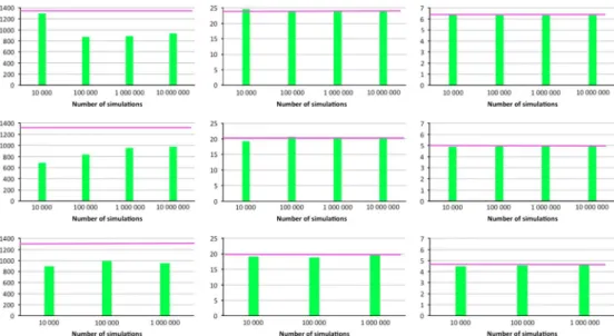
Figure 1. Convergence of the TVaR of Snat 99.5% for α=1.1, 2, 3 from left to right, for an

aggregation factorn=_{2, 10, 100 from up to down. The purple line corresponds to the analytical} value and the green plots are the average values obtained from the Monte Carlo (MC) simulations. They-scale gives the normalised TVaR (TVaRn/n) and is the same for each column.

Let us now analyse the diversification benefitDκ(Sn) associated with TVaR, denoted byDn. We use

the results (16) and (15) to compute it explicitly and then check the convergence of the MC. The same parameter set and the same simulations are used to produce the numbers displayed in Figure 2. As expected, the convergence of the diversification benefit follows a similar pattern as for the TVaR. Indeed, we see in Figure 2 that:

∙

The diversification benefitDnofSnincreases withn

∙

Dnincreases withα

∙

The rate of convergence ofDnincreases withn

∙

The heavier the tail, the slower the convergence

Table 1. Relative errors (when comparing results obtained by Monte Carlo and analytical ones) of theTVaRnand the diversification benefitDnforSn, at 99.5% and for variousα, as a function of the aggregation factorncomputed with one million simulations.

n=_{2 (%) n}=_{10 (%) n}=_{100 (%)} α=_1.1 TVaRn −33.3 −27.3 −26.9 Dn 1,786 742 653 α=₂ TVaRn 0.38 0.14 0.05 Dn −2.61 −0.44 −0.14 α=₃ TVaRn 0.30 0.14 −0.10 Dn −1.30 −0.25 0.15

Figure 2. Convergence of the diversification benefit of Sn (associated with TVaR at 99.5%) for α=_{1.1, 2, 3 (from left to right), for an aggregation factorn}=_{2, 10, 100 (from up to down). The} purple lines are for the analytical values and the green ones are the average values obtained from the Monte Carlo (MC) simulations. They-scale is the same for all the graphs, for fair comparison.

∙

In the case of very heavy tail and strong dependence (α=_{1.1 and θ}=_{0.91), we do not see any} satisfactory convergence, even with ten million simulations, and for anyn

∙

When α=_{2, 3, the convergence is good from one million, 100,000 simulations onwards,} respectively.

Forα=_{1.1, the convergence is poor. In this case, we see an overestimation of the diversification} benefit that is above 600% for all aggregation factors includingn=_{100 (see Table 1). This significant} overestimation may seem high, however, the impact is not material since we are talking here of very small diversification benefit of the order of a few percents (3.6% forn=_{10, for instance). We see in} Figure 2 that the diversification benefit does not converge in all cases. Obviously, ten millions simulations are not sufficient to ensure a good convergence. The reason is that MC samples the space evenly, whereas, in this case, we would need much more points in the tails to see a good convergence. In Table 1, we present the results of a convergence study as a function of the aggregation factor. The number of simulations is fixed at one million and we vary the aggregation factor n. We see a decreasing estimation error by MC when increasing the aggregation factor, with small errors for

α=_{3 and 2 and substantial errors for very fat tails and strong dependence. In the latter, we also see a} systematic underestimation of the TVaR and an overestimation of the diversification benefit, whatever the aggregation factor. Such a fact is not surprising for very fat tails (αclose to 1). With the thinner tails and lower dependence, MC has a tendency to overestimate the TVaR and underestimate the diversification benefit except forn=_{100. Note that the error decrease is large between 2 and 10,} but much smaller afterwards.

3.2. Weibull marginals with Gumbel survival copula

Here we use Theorem 2.2 and Corollary 2.2 to compute the TVaR and the diversification benefit, for various values of the aggregation factorn(2, 10, 100). Recall that in this example,θ=2=1/τ, which means that the tail index isfixed toα=_{2. Only the scaling parameter cof the Weibull marginals} might be modified, but for the sake of simplicity, wefix it to 1.

As in the previous example, we compare the values obtained analytically with those obtained via MC simulations, considering ten sets of simulations for our set of parameters, varying the number of simulations per run from 10,000 to ten millions (except forn=_{100, where we stop at one million} due to computer limitations). We report here the average values of the ten sets and verify that the standard deviation is decreasing with the number of simulations.

We present in Figure 3 the normalised TVaR,TVaRn/n (as we do it for Pareto–Clayton), for the

three casesn=_{2, 10, 100. We observe that:}

∙

TVaRn/ndecreases withn.

∙

TVaRn/n decreases faster between n=2 and n=10 (−29%) than between n=10 andn=100 (−12%).

∙

The rate of convergence is good in all the cases and the deviation reaches <_{1% already with} 100,000 simulations.

On thefigure, the convergence is very clear. The absolute value of the relative error is<_{2% for both} risk measures and for alln’_{s. The convergence, reached already with 100,000 simulations, is faster} than the one obtained with the Pareto–Clayton model. This is explained by the fact that, for 0<τ<1, the Weibull marginals are moderately heavy tailed and the Gumbel survival copula has a

much weaker dependence in the tail compared to the Clayton survival copula; indeed recall that a Clayton copula has lower tail dependence (hence theflipped Clayton copula, as here, will exhibit only upper tail dependence), whereas the Gumbel one has upper tail dependence (the survival copula of Gumbel form will then exhibit only lower tail dependence). Thus, the simulation requires less points to model accurately the behaviour in the tails. Increasing the number of aggregation improves the con-vergence. Indeed, when measuring the variation with one million simulation for the TVaR, we see that forn=_{2 we have an underestimation of 0.65%, which decreases to 0.18% forn}=_{100. Beside the gain} in precision, the analytical formula can be numerically evaluated 65 times faster, respectively, 75 times faster (forn=_{10, respectively,n}=_{100 for one million simulation), than the estimation given by MC} method. Moreover, MC method cannot be used for higher number of aggregation (i.e.n=10,000) due to lack of system memory, while it is of course feasible for the analytical formula.

In Figure 4, we present the results for the diversification benefitDn, when choosing TVaR as risk

measure. Similar comments hold forDnas forTVaRn/n. The convergence is already very good for

10,000 simulations. We also observe, as expected, thatDnincreases withn, as it is the case for the

Pareto–Clayton model.

4. Diversification Benefit as a Function of the Aggregation Factor and the Risk

Measures, for Various Types of Models

The diversification benefit is an important parameter for determining the efficiency of the use of capital of an insurance company. It plays a crucial role in the new risk disclosure of companies. Unfortunately, it is a quantity that has attracted little attention of researchers because it is not a universal measure: it depends on the number of underlying risks in the definition, as well as on the choice of the underlying risk measure (see Emmer et al., 2015). However, this parameter can be Figure 3. Convergence of the normalised TVaR of Sn, TVaRn/n, at 99.5% for c=1, τ=1

2 and

θ=_{2, for an aggregation factor n}=_{2, 10, 100 from left to right. The purple line corresponds to} the analytical value and the green plots are the average values obtained from the Monte Carlo (MC) simulations. They-axis is the same for the three plots.

Figure 4. Convergence of the diversification benefit Dn ofSn (associated with TVaR at 99.5%)

for c=_{1, τ}=1

2 andθ=2, for an aggregation factorn=2, 10, 100 from left to right. The purple lines are for the analytical values and the green ones are the average values obtained from the Monte Carlo (MC) simulations. They-axis is the same for the three plots, for fair comparison.

studied as a function of the number of risks, as well as of the risk measure. It is what we aim at doing here, addressing in particular the question of the impact of the existence of dependence among risks on the behaviour of the diversification benefit. In a previous paper (see Busse et al., 2014), we explored analytically the limit of diversification when introducing a systematic risk in the model through a latent rv common to all risks in the portfolio. Here we tackle again the problem, but in a different way, using various dependence models and, as in Busseet al. (2014), comparing it to the independent case. We also study the effect of light and heavy tailed marginals.

When assuming dependence, we consider our two previous models, Pareto–Clayton and Weibull– Gumbel. We add two cases, one with independent Pareto rv’s, to evaluate the impact of the dependence, and one considering a multivariate Gaussian model to evaluate the impact of the tail thickness. All chosen examples share the existence of anaytical expressions for the risk measures and, as consequence, for the diversification benefit. We can then compare the behaviour of the diversification benefit as a function of the aggregation factorn(fromn=_{2 to 10,000) and the risk measures, TVaR} and VaR. Since both are used in practice, it is interesting to see if the choice of risk measure has an influence on the diversification benefit.

Note that for comparison purpose, we choose the Pareto–Clayton case withα=2, since it corre-sponds to the tail index of the Weibull–Gumbel model. For completness, we also recall briefly the evaluation of the diversification benefit in the two additional examples, independent Pareto and mutivariate Gaussian risks.

4.1. Independent Pareto rv

’

s case with asymptotic threshold

ð

κ

%

1

Þ

To avoid computations, we are going to look only for approximations when considering extreme quantiles (i.e. when the thresholdκtends to 1), for which Feller’s result (see Feller, 1966) is available. For sharper and not necessarily asymptotic results, computations could be done using the Normex method (see Kratz, 2014).

Feller has shown that the tail distribution of the sum of independent rv’s with regularly varying (RVα) tail

distribution is asymptoticallyRVα. Applying this result when considering iid Pareto-(α,β) rv’s provides

qn=VaR_κð ÞSn =F_S nð Þ κ _κ!1β 1 κ n 1=α 1 ! (27) and TVaRκðSnÞ κ_!1 nβα 1 κ ð Þðα 1Þ´ αqn+_β qn+_β ð Þακ_!1β α α 1 1 κ n 1=α 1 ! (28)

It gives back the well known asymptotic relationTVaRκ/VaRκ→ α/(α−1) asκ→ 1.

Now let us look at the diversification benefit for high thresholdκ. When choosing the VaR as risk measure (q1satisfying (6)), we have

D nð Þκ =1 qn nβ α 1 n q1 β α 1 κ!11 n1α 1ð1 κÞ 1=α 1 n 1 α 1 1 κ ð Þ 1=α 1 1 α 1 (29)

and for the TVaR, Dnð Þ κ κ_!11 α α 1n 1 α 1ð1 κÞ 1=α 1 n α11 α α 1ð1 κÞ 1=α 1 1 α 1 (30) from which we deduce the asymptotic limit asκ → 1, which is the same for both risk measures, as

expected: lim κ!1D nð Þκ =lim κ!1Dnð Þκ =1 n ð1 1=αÞ (31) which tends to 1 asn _→ ∞.

Note that in the Gaussian case,Dn(orDn), converges also to 1 asn → ∞with a rate of convergence

ofn1/2_{, and not only for high thresholdκ.}

4.2. Multivariate Gaussian distribution

Consider the Gaussian vector (Xi)i=1,…, nwith expectation vector (μi)i=1,…, n,μi=μ, and

(non-negative definite) covariance matrix Γ=(γij)1≤i, j≤n such that γii=σ2, ∀i. ThenSn=Pn_i

=1Xi is

normally distributed with mean nμ and variance nσ2+2P₁

≤i<j≤nγij. Hence, with the notation rij=corr(Xi,Xj) andϕ,Φ, for the standard normal pdf, cdf, respectively, we can write

qn=VaR_κð ÞSn =n_μ+Φ 1_{ð Þκ} ffiffiffi n p σ ffiffiffiffiffiffiffiffiffiffiffiffiffiffiffiffiffiffiffiffiffiffiffiffiffiffiffiffiffiffiffiffi 1+2 n X 1≤i<j≤n rij s ≤nμ+Φ 1_{ð Þκ σ} =n q1

whereas, for the TVaR, TVaRκðSnÞ=nμ+ ϕΦ 1ð Þκ 1 κ ffiffiffi n p σ ffiffiffiffiffiffiffiffiffiffiffiffiffiffiffiffiffiffiffiffiffiffiffiffiffiffiffiffiffiffiffiffi 1+2 n X 1≤i<j≤n rij s ≤n μ+ ϕΦ 1ð Þκ 1 κ σ ! =n TVaR_κð ÞX We deduce that Dn=D_n=1 1 ffiffiffi n p ffiffiffiffiffiffiffiffiffiffiffiffiffiffiffiffiffiffiffiffiffiffiffiffiffiffiffiffiffiffiffiffi 1+2 n X 1≤i<j≤n rij s ≥0 ð Þ

The diversification benefit can tend to any constant between 0 and 1, asn → ∞, whenever there

exists a linear dependence between the components. For instance, ifrij=r≠0, ∀i≠j, the diversifi

-cation benefit reduces to

Dn=D n=1 1 ffiffiffi n p ffiffiffiffiffiffiffiffiffiffiffiffiffiffiffiffiffiffiffiffiffiffiffi 1+ðn 1Þr p

when r=_{1 (full comonotonicity), Dn}=D_n=0, whereas for r=0 (independent case), we obtain Dn=D_n=1 n 1=2, which is also the limit (asκ _→ 1) of the diversification benefit given in (31) for independentα-Pareto rv’s withα=_2.

Let us compare the diversification benefit as a function of n, for both TVAR and VaR, for high threshold κ=_{99.5%, considering the following cases: (i) independent α-Pareto with α}=_2, (ii)α-Pareto margins and survival Clayton (θ) copula (Pareto–Clayton) withα=₂=_{1/θ, (iii)} Gaus-sian margins and GausGaus-sian copula (GausGaus-sian–Gaussian) with (linear) correlationr=_{0.42 estimated} on the previous Pareto–Clayton model, (iv) τ-Weibull margins and Gumbel (θ) copula (Weibull–Gumbel) withθ=₂=_{1/τand (v) Gaussian}–Gaussian with correlationr=_{0.39 estimated on} the Weibull–_{Gumbel model.}

Note that the linear correlation coefficients r are estimated from the realisation of the simulated model. Moreover, the number of simulations is chosen such that the Kendall-τestimate corresponds to the theoretical one. Recall that the theoretical value ofτ, as a function of theθparameter of the copula, is known for both Clayton, withτ= θ

θ+2, and Gumbel, with 1 1

θ. The convergence is then

reached with 100,000 simulations.

In Table 2, we present the results obtained onDnandDnusing analytical formulas for all of them, and not simulations. Note that it completes the numerical application for the analytical diversifi -cation benefit done in the previous sections with the TVaR only. Moreover, the functionsD

nofnare plotted in Figure 5 for the various models.

Table 2. Analytical diversification benefit ofSn,DnandDn, at 99.5% as a function of the

risk measures TVaR and VaR, respectively, and of the aggregation factorn.

n=2 (%) n=10 (%) n=100 (%) n=1,000 (%) n=10,000 (%) Independent Pareto Dn=D n 29.3 68.4 90.0 96.8 99.0 Pareto–_Clayton Dn 13.2 25.5 28.6 29.0 29.0 D n 12.9 25.2 28.3 28.6 28.7 Dn=Dn 1.021 1.014 1.012 1.012 1.012 Gaussian–Gaussian r=_{0.42 (Clayton)} Dn=D n 15.7 30.9 34.7 35.1 35.2 Weibull–_Gumbel Dn 23.1 47.0 54.1 54.8 54.9 D n 19.6 40.4 46.5 47.2 47.2 Dn=Dn 1.179 1.162 1.163 1.163 1.163 Gaussian–Gaussian r=_{0.39 (Gumbel)} Dn=D n 16.6 32.8 37.1 37.5 37.5

Note: Tail indexα=2, survival Clayton parameterθ=1/2, Weibullτ=1/2, Gumbel para-meterθ=_2. 100.0% 80.0% 60.0% 40.0% 20.0% 0.0% 1 10 100 1’000 10’000

Figure 5. Plot of the diversification benefitD

n (y-axis) as a function ofn (x-axis), forVaRκ with κ=99.5%. The curves from bottom to up correspond, respectively, to Pareto (α=2)-Clayton (θ=_{1/2), Gauss-Gauss (Clayton; r}=_{0.42), Gauss-Gauss (Gumbel; r}=_{0.39), Weibulll (τ}= 1/2)-Gumbel (θ=_{2), independent Pareto (α}=_{2) and Gauss models.}

We show in Table 2 and Figure 5 that:

∙

The dependence has a significant impact on the evolution of the diversification benefit withn, as expected. In the case of dependence, the diversification benefit levels off rapidly, already at n=100, while for the independence case, it still increases fromn=100 ton=10,000.

∙

The evolution of the diversification benefit is similar for the two underlying structures, increasing and levelling off withn, for both. For example, in the dependent case, fromn=_{2 to 10, it increases} approximately by a factor 2 (1.9 for Pareto–Clayton and 2.0 for Weibull–Gumbel), regardless of the risk measure used to compute the diversification benefit.

∙

Although both evolutions are the same fromn=_{2 to 100, the Pareto}–Clayton model exhibits a stronger tail dependence and a fatter tail than the Weibull–Gumbel one. This appears through the difference of the diversification benefit between the two models, almost twice bigger for the second.

∙

We see in the table that the diversification benefit computed with the VaR is always lower than the one computed with the TVaR. This is to be expected, since the latter risk measure takes into account the whole distribution beyond afixed threshold (for instance, 99.5% in this case), whereas the VaR only looks at one point of the distribution. However, the difference is more pronounced for the Weibull– Gumbel model than the Pareto–Clayton one, with a ratio of the order of 1.2 instead of 1.01, respectively.

∙

The ratioDn/Dn*stabilises fromn=10 onwards, with 1.012 for Pareto–Clayton and 1.163 for

Weibull–Gumbel. Starting at n=100, the diversification benefit does not change anymore. It is interesting to note that the more dependence in the tails (Clayton copula), the less difference between the diversification benefit measured with TVaR or VaR. Nevertheless, this difference is never very large (<_20%).

∙

Comparing the results obtained with the Pareto–_{Clayton model and the corresponding Gaussian}– Gaussian one, emphasises that the tail dependence associated with a fat tail limits the diversification benefit. The diversification benefit limit is 35.2% for the Gaussian case, while it is only 29% in the Pareto–Clayton case.

∙

The comparison leads to a different result in the Weibull–Gumbel case and the Gaussian one. Here we see much stronger diversification benefit for the Weibull–Gumbel model than for the Gaussian– Gaussian one. The intuition to explain this observation being less obvious than with the previous model, varying the parameters (as in Sarabiaet al., 2017) would help to analyse this effect. Let us just note that the linear correlation implied byθ=2 is quite high in this case.

∙

As expected, 100% diversification benefit is reached in the independent case only.

5. Conclusion

The purpose of this study is to explore new ways of validating internal models. As mentioned in the introduction, it is not possible to validate statistically a VaR at a threshold of 99.5%, which represents a probability of 1 over 200 years. Thus, we need to resort to indirect ways, testing various aspects of the model. Here we test the convergence of MC algorithms for aggregated risks in presence of both heavy tailed marginals and non-linear dependence in the tails. We also explore the behaviour of the diversification benefit as a function of: the number of risks, the type of marginal distributions, the dependence structure and the choice of risk measure used to evaluate it. This is done after having derived explicit formulas for both the risk measures and the diversification benefit.

To test the MC algorithm, we consider two standard examples of dependence structure and marginal distributions, Pareto–Clayton and Weibull–Gumbel. We obtain via mixing techniques explicit

formula for the aggregated pdf for both examples. By varying the number of simulations from 10,000 to 10 millions, we observe that for Pareto(α)–_{Clayton(1/α), a minimum of 100,000} simu-lations is needed to obtain a good convergence for moderately heavy tails and moderate tail dependence (α=2 or 3). For very heavy tails and moderate tail dependence (e.g.α=1.1), we do not reach convergence, even with ten millions simulations, showing that the results obtained by MC method for this kind of distributions must be considered carefully. The second case is more limited since the Gumbel copula parameter isfixed toθ=_{2. However, we can conclude that the convergence} with a Gumbel copula is faster than with a Clayton survival copula, since 100,000 simulations are enough for moderate heavy tailed Weibull marginal distribution.

When studying the behaviour of the analytical diversification benefit of Snas a function of the

aggregation factorn, we observe that the dependence structure matters more for the diversification benefit than the type of marginals do. It is interesting to note that in the independent case, the diversification benefit is identical in the limit, when the threshold tends to 1, for Pareto withα=_{2 or} Gaussian risks, despite the fact that Pareto has a heavier tail. We see that Gaussian marginals with Clayton or Gumbel copula have a lower diversification benefit than independent Pareto risks, or than Weibull marginals with Gumbel copula. Withn=_{100, the diversification benefit saturates in all the} cases except for independent Gaussian (or Paretoα=2) risks; in this latter case, it gets close to 100% only whenn>10,000. Another interesting effect is that the diversification benefit depends little on the choice of risk measure for Pareto–Clayton (change around 2%), while in the Weibull–Gumbel case, the change can go up to 20%. It is a question we will explore further when consideringαandθ

independently.

Replacing MC simulations by explicit expressions is a considerable gain in precision and time. Indeed, the analytical formulas are estimated to be 40–500 times faster than MC method, with the time difference increasing with increasing number of aggregated variables. Moreover, with the analytical formula, we can estimate the TVaR even for very heavy tailed distributions whenever MC method fails even for ten millions simulations. Explicit formulas allow us to explore the aggregation behaviour of the risk measures and the diversification benefit. It is a precious tool for validating results of internal models, which are based on MC simulations. This study is afirst step towards a general approach where we could choose the tail index and the copula parameter independently. It will be the object of further investigation.

Acknowledgement

Partial support from RARE-318984 (an FP7 Marie Curie IRSES Fellowship) is kindly acknowledged.

References

Albano, M., Amdeberhan, T., Beyerstedt, E. & Moll, V.H. (2011). The integrals in Gradshteyn and Ryzhik. Part 19: the error function.SCIENTIA Series A: Mathematical Sciences,21, 25–42. Albrecher, H., Constantinescu, C. & Loisel, S. (2011). Explicit ruin formulas for models with

dependence among risks.Insurance: Mathematics and Economics,48(2), 265–270.

Bürgi, R., Dacorogna, M.M. & Iles, R. (2008). Risk aggregation, dependence structure and diver-sification benefit. In D. Rösch & H. Scheule (Eds.),Stress Testing for Financial Institutions (pp. 265–_{306), Riskbooks, Incisive Media, London.}

Busse, M., Dacorogna, M.M. & Kratz, M. (2014). The impact of systemic risk on the diversification benefits of a risk portfolio.Risks,2, 260–276.

Constantinescu, C., Hashorva, E. & Ji, L. (2011). Archimedean copulas infinite and infinite dimensions– with application to ruin problems.Insurance: Mathematics and Economics,49, 487–_495. Dacorogna, M. (2017). Approaches and techniques to validate internal model results. Available

online at the address https://papers.ssrn.com/sol3/papers.cfm?abstract_id=2983837 [accessed May 2017].

Dacorogna, M., Elbahtouri, L. & Kratz, M. (2015–2016). Explicit diversification benefit for dependent risks, ESSEC WP 1522 (2015) & SCOR Paper 38.

Emmer, S., Kratz, M. & Tasche, D. (2015). What is the best risk measure in practice? A comparison of standard measures.Journal of Risk,18(2), 31–60.

Feller, W. (1966). An Introduction to Probability Theory and its Applications (Vol. II). Wiley, New-York.

Gradshteyn, I.S. (1988). Tables of Integrals, Series, and Products, Academic Press, San Diego. Hashorva, E. & Ji, L. (2014). Random shifting and scaling of insurance risks.Risks,2, 277–288. Kohl, K.T. & Moll, V.H. (2011). The integrals in Gradshteyn and Ryzhik. Part 20: hypergeometric

functions.SCIENTIA Series A: Mathematical Sciences,21, 43–54.

Kratz, M. (2014).Normex, a new method for evaluating the distribution of aggregated heavy tailed risks. Application to risk measures. Extremes17(4), Special issue on Extremes and Finance (Guest Ed. P. Embrechts), 661–691.

Marshall, A.W. & Olkin, I. (1988). Families of Multivariate Distributions.Journal of the American Statistical Association,83, 834–841.

Oakes, D. (1989). Bivariate Survival Models Induced by Frailties.Journal of the American Statistical Association,84, 487–493.

Sarabia, J., Gómez-Déniz, E., Prietoa, F. & Jordá, V. (2017). Aggregation of Dependent Risks in Mixtures of Exponential Distributions and Extensions. Available online at the address https:// arxiv.org/abs/1705.00289 [accessed May 2017].

Appendix

We provide the proofs of the analytical results given in section 2. For further details, we refer to Dacorognaet al. (2015–_2016).

A. Proofs of the results given for the Pareto–Clayton model

∙

Proof of Proposition 2.1

The proof relies mainly on the application of the Oakes–Marshall–Olkin Theorem, which makes the computations offneasier.

As given in Marshall & Olkin (1988), choosingH(x)=_e−x_{forx>0, and the latent rvΘa GammaΓ(α;} β) rv with shape parameter α>_{0 and rate parameter β}>_{0 (or scale parameter 1/β) with pdf} fΘðxÞ= β

α

Γ_{ð Þ}α x α 1_e βx

x≥0

ð Þ, allows to check that the model defined by (2) and (3), which corresponds to our

model, satisfies (1) by the Oakes–Marshall–Olkin Theorem (see Dacorognaet al., 2015–2016). Since conditioningXbyΘ_{transforms the dependent risks into independent conditional ones, we write}

the pdffnofSnas

fnð Þs = ð1

0

With the choice ofHandΘ_{, our model satisfies (1), hence the conditional rv}’_sXi|Θ=_θ,i=_1,…_{,n, are} i.i.d. exponentially distributed with parameter θ. We deduce that their conditional sum Sn=Pn_i

=1Xi j Θ=θisΓ(n,θ)-distributed. So we obtain immediately that the pdf ofSnis the one of

a compoundγdistribution and is given by fnð Þs =s n 1 Γ_{ð Þn} ð1 0 θne sθ β α Γ_{ð Þα} θ α 1_e βθ_d θ= Γð_α+nÞ Γ_{ð Þα}Γ_{ð Þn} ´ βαsn 1 β+s ð Þα+n hence the result (8).

∙

Proof of Theorem 2.1

Using the definition of TVaR and Proposition 2.1, we obtain TVaRn= 1 1 κ ð1 qn s fnð Þs ds= β 1 κ ð ÞBðα;nÞ ð1 qn β sn _1+s ð Þ α nds (32)

The change of variablesu=_{(1 +s)}−1_{in (32) gives (11).}

Using the definition of TVaR and Proposition 2.1 withn=_{2, gives} TVaR2=α 1 +_α ð Þβα 1 κ ð₁ q2 s2 β+s ð Þα+2ds from which (13) follows, via the change of variablesu=_s/β.

Now let us assume thatα2Nn f0;1g. We prove (12) by induction onα. Forα=_{2, computing (11) provides}

TVaRn= β 1 κ ð ÞBð2;nÞB pnð ;1;n+1Þ= βn nð +1Þ 1 κ ´ 1 ð1 pnÞn+1 n+1 = nβ 1 κ 1 ð1 pnÞ n+1

which corresponds to (12) when replacingαby 2.

Assume now that (12) is satisfied for any 2≤α≤k (and for anyn≥1). Let us prove that it holds forα=k+ 1. It comes back to prove the induction on the following expression of the incomplete

βfunction: B pnð ;k;n+1Þ= ðk 1Þ!n! n+k 1 ð Þ!B pnð ;1;n+kÞ Xk 1 j=1 k 1 ð Þ!n! n+k j ð Þ!j! p j nð1 pnÞ n+k j But, sinceB pnð ;1;n+kÞ= 1 n+k 1 ð1 pnÞ n+k ; B pnð ;k;n+1Þ=ðk 1Þ!n! n+k ð Þ! X k 1 j=0 k 1 ð Þ!n! n+k j ð Þ!j!p j nð1 pnÞ n+k j ₍₃₃₎

It is immediate to check that (33) is satisfied for k=_{2. Then, assuming that (33) holds for} k2Nn f0;1g(and anyn≥1), we check that it remains true fork+ 1. An integration by part gives

B pnð ;k+1;n+1Þ= 1 n+1p k nð1 pnÞ n+1 + k n+1B pn;k;n +2 ð Þ

Under the inductive assumption, we can apply (33) to expressB(pn;k,n+ 2); replacing it in the

∙

Proof of Corollary 2.1

i. It is immediate knowing the fact thatEð ÞX = β

α 1forX(α,β)-Pareto distributed. ii. Combining (10) with (11) in the definition ofDngives (15).

For the case n=2, (16) can be directly deduced from (15). An alternative, with simpler computation, is to deduce (16) from (13) and the definition (4) of the diversification benefit. B. Proofs of the results given for the Weibull–Gumbel model

∙

Proof of Proposition 2.2

The proof of this proposition is based on mixing techniques and on the following technical lemma. Lemma B.1Forn≥1, we have

∂n_se cpffiffi_s = c_ð 1_ÞnΓ n 1 2 2 ffiffiffi π p s12 ne c ffiffis p 1F11 n;2 2n;2cpffiffi_s

where∂sdenotes the partial derivative w.r.t.s.

Proof of Lemma B.1. We proceed by induction.

For n=_{1, Lemma B.1 is well satisfied since} ∂s e c

ffiffi s p = c 2s 1=2_e cpffiffi_s , Γ_ð1=2Þ=pffiffiffiπ, and 1F1(0, 0;z)=1, for all realz. Suppose now that Lemma B.1 is true forn≥1 and let us check it for

n+ 1. Under the induction assumption, we have ∂n+1 s e c ffiffi s p =cð 1Þ n_Γ n 1 2 2 ffiffiffi π p ∂s s 1 2 n_e c ffiffis p 1F1 1 n;2 2n;2c ffiffi s p Let us compute Anð Þs : =∂s s12 ne c ffiffis p 1F1 1 n;2 2n;2cpffiffi_s ð Þ

, using the following properties of hypergeometric functions (see, e.g. Gradshteyn, 1988):

i. ∂zð1F1ða;b; zÞÞ=a b1F1ða+1;b+1; zÞ ii. 1F1_ða;2a; z_Þ=ez=20F1 a+1 2;z 2 16 iii. 1F1ða;2a 1; zÞ=1 4ez=2 40F1 a 12; z 2 16 +z Γ a 1 2 ð Þ Γa+1 2 ð Þ0F1 a+12;z 2 16 iv. 0F1ða; zÞ=e 2 ffiffiz p 1F1 a 1 2;2a 1; 4 ffiffiffi z p

where0F1(a;x) is the confluent hypergeometric function defined by 0F1ða; zÞ=P1k=0ð Þa1k

zk k! withð Þak= Γ_ða+kÞ Γð Þa We have Anð Þs =1 2s n_e cpffiffi_s c1F12 n;3 2n; 2cpffiffi_s c+ð2n 1Þs 1=2 1F11 n;2 2n; 2cpffiffi_s h i =1 2ð1 2nÞs n 1=2 0F1 1 2 n; c2_s 4 =1 2ð1 2nÞs n 1=2_e cpffiffi_s 1F1 n; 2n; 2c ffiffis p

using (i) in thefirst equality, then both (ii) and (iii) in the second one, and (iv) in the last one. We can

conclude that Lemma B.1 is satisfied forn+ 1. □

Forn≥0 anda;b2R(see, e.g. Albanoet al., 2011), we have In;bð Þa = ð1 0 xn 1=2e ax b=xdx=ð 1Þn∂n_a I0;bð Þa with I0;bð Þa = ð1 0 x 1=2e ax b=xdx= ffiffiffi π a r e 2pffiffiffiffiab ð34Þ

when differentiatingIn,b(a) with respect to the parametera.

Let us prove now Proposition 2.2. As given in Marshall & Olkin (1988), it is enough to choose H(x)=_e−x_{(x>0) andΘa Lévy-distributed (0,c}2_{/2) positive rv withc>0, and pdff}

Θð Þx = c

2pffiffiffiffiffiffi_πx3e

c2 4x,

forx≥0, then to apply the Oakes–Marshall–Olkin theorem.

Computing the Laplace transform ofΘ_{via the change of variablesu}=_θ−1_{, gives}

LΘð Þt = ð1 0 e θt_f Θð Þθ dθ=I0_;tc2=4=e c ffiffi t p

So, with this choice ofH, the marginal distribution defined in (3) satisfiesLΘð lnHðxÞÞ=e c

ffiffi

x

p

. It corresponds on (0,∞) to the survival cdf of a Weibull (c, 1/2) defined in (17). Hence we obtain the marginal distributions of our model.

Now, since the generator of the Archimedean survival copula defined in (2), is given by

ϕð Þt =LΘð Þt 1=

1

c2ð lnð Þt Þ 2

we deduce the structure of dependence assumed in our model, namely (19) when taking the para-meterθ=_2.

For the 2nd part of the proof, we can write, as in the proof of Proposition 2.1, fnð Þs = ð1 0 fSnjΘð Þs fΘð Þθdθ= c s n 1 2 ffiffiffi π p _Γ n ð Þ ð1 0 θðn 1Þ 1=2e sθ c₄2_{θdθ (35)}

Therefore, using (34) provides fnð Þs = c s n 1 2 ffiffiffi π p _Γ n ð Þð 1Þ n 1 ffiffiffi π p ∂n_s 1s 1=2_e cpffiffi_s = s n 1 Γ_{ð Þn} ð 1Þ n ∂n_se cpffiffi_s

Applying Lemma B.1 allows to conclude.

∙

Proof of Theorem 2.2

By definition of the TVaR, we can write, using the expression (35) forfn

TVaRn= 1 1 κ ð1 qn s fnðsÞds= c 2 ffiffiffi π p 1 κ ð ÞΓ_{ð Þn} ð1 0 θn 3=2e c42θ ð1 qn sn_e sθ_{ds d} θ

But we have, by the change of variablet=_sθ

ð1 qn sne sθ_ds= 1 θn+1 Γðn+1; θqnÞ= n!e θqn θn+1 X n k=0 θqn ð Þk k!

Γ_{(s; x) denoting the incomplete γ function defined by} Ð1

xts 1e tdt that can be expressed as a discrete sum (see Gradshteyn, 1988).

So we deduce that TVaRn= c n 2 1ð κÞ ffiffiffi π p ð1 0 1+_θqn ð Þθ 5=2e 4c2θ θqn_dθ+X n k=2 qk n k!Ik 2;c2=4ð Þqn ! = c n 2 1ð κÞ ffiffiffi π p I1;qn c 2₌₄ +qnI0_;q n c 2₌₄ +X n k=2 qk n k!Ik 2;c2=4ð Þqn !

using the definition (34) in thefirst equation, and the change of variableθ=u−1_{to compute the}

integral, in the second one. On one hand, we haveI0;qn c

2₌₄

=2 ffiffiπ p

c e

cpffiffiffiffiqn_{; on the other hand, a straightforward computation}

givesI1;qn c 2₌₄ =4 ffiffiπ p c3 e c ffiffiffiffi qn p 1+cpffiffiffiffiffi_qn

. Moreover, we can write, using once again (34) Ik 2;c2₌₄ð Þqn =ð 1Þk∂k_q 2 n I0;c2=4ð Þqn =ð 1Þk 12 ffiffiffi π p c ∂ k 1 qn e cpffiffiffiffiqn

from which we deduce, applying Lemma B.1, that

Xn k=2 qk n k! Ik 2;c2=4ð Þqn =q 3=2 n e c ffiffiffiffi qn p Xn k=2 Γ k 3 2 k! 1F1 2 k;4 2k; 2c ffiffiffiffiffi qn p ð Þ

Combining these results provide (22). Applying (22) withn=_{1 providesTVaR1}=2e

cpffiffiffiq₁ 1 κ ð Þc2 1+c q 1=2 1 + c2_q 1 2

, from which (23) follows since q1=ðlnð1 _κÞÞ2=c2. Forn=_{2, (24) is a direct application of (22).}

∙

Proof of Corollary 2.2

i. It is immediate knowing thatEð ÞX =cΓ ₁+1

τ

=2cwhenXis (c,_τ)-Weibull distributed. ii. Combining (22), (24), respectively, with (23) in the definition of the diversification benefit (4)