GloVeNoR - Global Vectors for Node Representations

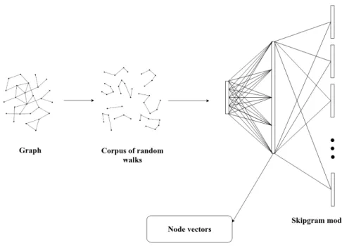
San Jose State University

SJSU ScholarWorks

Master's Projects Master's Theses and Graduate Research

Spring 5-22-2019

GloVeNoR - Global Vectors for Node

Representations

Shishir Kulkarni

San Jose State University

Follow this and additional works at:https://scholarworks.sjsu.edu/etd_projects

Part of theArtificial Intelligence and Robotics Commons, and theOther Computer Sciences Commons

This Master's Project is brought to you for free and open access by the Master's Theses and Graduate Research at SJSU ScholarWorks. It has been accepted for inclusion in Master's Projects by an authorized administrator of SJSU ScholarWorks. For more information, please contact [email protected].

Recommended Citation

Kulkarni, Shishir, "GloVeNoR - Global Vectors for Node Representations" (2019).Master's Projects. 722. DOI: https://doi.org/10.31979/etd.axu4-hswg

GloVeNoR - Global Vectors for Node Representations

CS298 Report

Presented to

Department of Computer Science San Jose State University

In Partial Fulfillment

of the Requirements for the Degree Master of Science

By

Shishir Kulkarni May, 2019

c

○2019 Shishir Kulkarni ALL RIGHTS RESERVED

The Designated Project Committee Approves the Project Titled

GloVeNoR - Global Vectors for Node Representations

by

Shishir Kulkarni

APPROVED FOR THE DEPARTMENTS OF COMPUTER SCIENCE

SAN JOSE STATE UNIVERSITY

May 2019

Dr. Katerina Potika Department of Computer Science Dr. Sami Khuri Department of Computer Science Dr. Mike Wu Department of Computer Science

ABSTRACT

A graph is a very powerful abstract data type that can be used to model entities (nodes) and relationships (edges). Many real world networks like biological, computer and friendship networks can be represented as graphs. Graphs can be mined to extract interesting patterns and interactions between the participating entities. Recently, various Artificial Intelligence (AI) and Machine Learning (ML) techniques are used for this purpose. In order to do that, the nodes of a graph have to be represented as low dimensional feature vectors. Node embedding is the process of generating a

𝑛-dimensional feature vector corresponding to each node of a graph, such that the structurally similar nodes remain close in the𝑛-dimensional space.

There are many state-of-the-art methods, like node2vec and DeepWalk to com-pute node embeddings. These techniques borrow methods like the Skip-Gram model, used in the domain of Natural Language Processing (NLP) to compute word embed-dings. This project explores the idea of porting the GloVe (Global Vectors for Word Representation) model, a popular technique for word embeddings, to a new method called GloVeNoR to compute node embeddings in a graph. We evaluate the model’s quality by comparing it with node2vec and DeepWalk on the problem of community detection on five different data sets. We observe that GloVeNoR discovers similar or better communities than the other existing models on all the datasets.

ACKNOWLEDGMENTS

I would like to extend my sincerest gratitude towards my advisor, Dr. Katerina Potika for being a great source of guidance and inspiration in my masters project and my graduate degree. Her expertise in the domain of graphs and social networks helped me overcome all the difficulties that I faced while working on the project. Her resolute enthusiasm helped and inspired me to drive this project to a successful completion. I consider myself very fortunate to have her as my advisor and mentor.

I thank Dr. Sami Khuri and Dr. Mike Wu for being on my defense committee. I also thank them for their continued support and valueable feedback on the project. I would also like to thank Jay Katariya for helping me to perform experiments on different datasets and preparing a poster for the presentation.

Lastly, I would like to thank my parents and friends for having faith in me and being there. Their continued support made this journey a memorable one.

TABLE OF CONTENTS

CHAPTER

1 Introduction . . . 1

1.1 Graphs and Feature Learning . . . 1

1.2 Motivation and problem definition . . . 2

2 Terminology . . . 4

3 Related Work . . . 7

3.1 DeepWalk . . . 7

3.2 node2vec . . . 12

3.3 Deep neural networks for learning graph representations (DNGR) 18 3.4 Core2Vec . . . 22

4 GloVeNoR for node embeddings . . . 26

4.1 Background . . . 26

4.2 GloVe for word embeddings . . . 26

4.3 Proposed Algorithm - GloVeNoR . . . 28

4.4 An example of GloVeNoR . . . 29

5 Implementation and Experiments . . . 32

5.1 Implementation Details . . . 32

5.2 Zachary’s Karate Club dataset . . . 33

5.3 Harry Potter Dataset . . . 37

5.4 Facebook Dataset . . . 39

5.6 Astro dataset . . . 43

6 Conclusion and future work . . . 44

6.1 Conclusion . . . 44

6.2 Future Work . . . 45

CHAPTER 1 Introduction

1.1 Graphs and Feature Learning

Graphs are very powerful and expressive data structure used for representing a complex network of entities and relationships between them. For instance, a graph can be used to model protein-protein interaction networks in bioinformatics, a network of people on social media, a network of web pages and links amongst them on the internet, etc.

Graphs can be analyzed to extract useful information and patterns by studying the structural and functional roles of entities and relationships in it. In the past decade, Artificial Intelligence (AI) and Machine Learning (ML) techniques are being used to analyze graphs. However, these techniques require the input data to be represented as n-dimensional vectors of relevant features called feature vectors or embeddings. The quality of results depends on the number and quality of the selected features.

The task of selecting features using domain knowledge is called feature engineer-ing and is very difficult in the case of graphs because of their size and unordered nature. One solution to this problem is to use ML techniques for feature engineering itself. There has been a lot of research in the past few years focused on computing representation of graph entities using AI and ML models.

Most of this research suggests that methods used in Language modeling for ob-taining vector representation of words (word embeddings) can be applied to graphs with some tweaks. As a result, some state-of-the-art methods like node2vec [1] have

been developed which adopt a lot of techniques from the NLP domain. For in-stance, node2ve [1] borrows many of its concepts like the skip-gram technique from word2vec [2], a popular word embedding technique used for Natural Language Pro-cessing (NLP) applications. It is a predictive model that learns embeddings by trying to minimize the loss of predicting a word given another word.

There are other popular techniques [3] [4] in the NLP domain which follow a different approach for learning word embeddings. Using the node2vec philosophy, we research these techniques and examine their portability to graphs.

1.2 Motivation and problem definition

Global Vectors for Word Representation (GloVe) is a popular word embedding technique which uses linear arithmetic method and fundamental statistical properties of a text corpus for preserving semantic relationships between the words. Unlike word2vec, GloVe is transparent and uses global co-occurrence statistics which are fundamental to finding analogies amongst words. Compared to word2vec the model can be easily parallelized and is computationally inexpensive. The primary objective of this project is to port the GloVe algorithm to generate node embeddings of a graph. We use the embeddings to detect communities using the k-means clustering algorithm. We evaluate the generated communities using modularity and silhouette scores. We call our method GloVeNoR (Global Vectors for Node Representations).

This report is organized into6sections. The second section describes four popular node embedding techniques and their building blocks. It compares the inner working of these techniques with each other. The third section briefly discusses the GloVe algorithm used for word embedding. It also discusses GloVeNoR and the implemen-tation details. The fourth section talks about the datasets used for experimenimplemen-tation

and elaborates the results. The final section concludes the project and discusses the interpretation of results and future directions.

CHAPTER 2 Terminology

∙ Graph: A graph is formally defined as an ordered pair 𝐺(𝑉, 𝐸) where 𝐺 is the set of vertices and 𝐸 is the set of edges. Graphs are represented using adjacency matrix notation and adjacency list notation. An adjacency matrix is a 2D matrix of size |𝑉| × |𝑉|. If there is an edge between node 𝑖 and 𝑗, the value in the 𝑖𝑡ℎ _{row and 𝑗}𝑡ℎ _{column of the matrix is 1.}

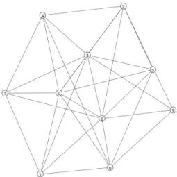
The adjacency list representation is an array of size |𝑉|. An element in the array represents a node in the graph and points to a list of the nodes that it is connected to. Figure 1 shows an example graph with 10 nodes. The adjacency matrix for the graph in Figure 1 is given by:

⎛ ⎜ ⎜ ⎜ ⎜ ⎜ ⎜ ⎜ ⎜ ⎜ ⎜ ⎜ ⎜ ⎜ ⎜ ⎜ ⎜ ⎝ 0 1 0 0 0 1 0 0 1 0 1 0 1 0 1 0 1 1 1 0 0 0 1 0 1 1 0 1 0 1 0 1 0 1 0 1 0 0 1 0 0 1 0 1 0 1 0 0 1 0 1 0 0 1 1 0 0 1 0 1 0 1 1 0 0 0 0 1 0 1 0 1 0 1 0 1 1 0 1 1 1 1 0 0 1 1 0 1 0 0 0 0 1 1 0 1 1 1 0 0 ⎞ ⎟ ⎟ ⎟ ⎟ ⎟ ⎟ ⎟ ⎟ ⎟ ⎟ ⎟ ⎟ ⎟ ⎟ ⎟ ⎟ ⎠

The adjacency list representation is given by: 0 : 1−>5−>8

1 : 0−>8−>4−>7−>6 2 : 1−>3−>6−>9 3 : 4−>9−>2−>7−>8 4 : 3−>5−>1−>8

Figure 1: Example Graph 5 : 3−>4−>8−>7−>0 6 : 1−>7−>9−>2 7 : 1−>6−>9−>3−>5−>8 8 : 0−>1−>7−>5−>4 9 : 2−>6−>7−>5−>3

∙ Directed and Undirected Graphs: If the edges of the graphs have a direc-tion, the graph is a directed graph. Otherwise, it is undirected. Figure 1 is an undirected graph. The adjacency matrix for undirected graphs is symmetric.

∙ Weighted and Unweighted Graphs: If the edges in a graph have a weight

associated with them, the graph is called a weighted graph. Otherwise, it is unweighted. Figure 1 is an unweighted graph. The adjacency matrix contains edge weights instead of 1 for weighted graphs.

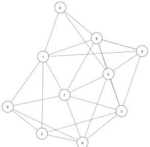
∙ Random Walk: A random walk is a stochastic process that describes a path consisting of successive random steps on a state space. For example, a random

walk on an integer number line will contain a sequence of numbers with an equal probability of moving to the left or right by 1 unit. A random walk can also be considered as a Markov chain. Figure 2 shows an example of random walks on a graph.

∙ Log-Bilinear model: In language modeling, a log-bilinear model is a model that predicts the representation of a word based on context words using lin-ear combination and computes the distribution of that word using similarity between prediction and representation of other words.

∙ Community Structure [5]: Community structure in a graph can be defined

as the grouping of the graph nodes into groups such that nodes within a group have denser connections with each other and sparser connections with nodes outside the group.

∙ Modularity[6]: Modularity is the difference between the probability of an edge present in a community 𝑖 and the probability of a random edge to be present in𝑖. Mathematically, it is expressed as:

𝑄= 𝑘 ∑︁ 𝑖=1 𝑒𝑖𝑖−𝑎2𝑖 where,

𝑒𝑖𝑖 = Fraction of edges present in community 𝑖,

𝑎𝑖 = Fraction of edges that have one end in community𝑖 𝑘 = number of communities

CHAPTER 3 Related Work

This chapter describes four state-of-the-art techniques used for computing node embeddings in a graph: node2vec, DeepWalk, DNGR, and Core2Vec. It also discusses the methods that these techniques use for extracting relationships between nodes of a graph.

3.1 DeepWalk

DeepWalk [7] uses deep neural networks for computing node embeddings. Deep-Walk has targeted applications to social network analysis and the authors of [7] state that it learns social representations of the nodes in a graph. The main contribution of the algorithm is that it uses deep learning in the domain of network analysis for the first time. The algorithm is performant, scalable and parallelizable. It can also be used with streaming data by making minor changes to the algorithm. [7] also presents experimental results of the algorithm’s performance on large social network-ing datasets on the multi-label classification problem.

The authors of [7] introduce the idea of using random walks to capture the relationships between nodes of a graph. A random walk [8] starting at vertex 𝑣𝑖 is

denoted by 𝑊𝑣𝑖. The length of the walk 𝛾 is a hyperparameter. A state at any time

in a random walk is given by random variables𝑊𝑣𝑖1, 𝑊_𝑣𝑖2...These variables represent

the stochastic probability of selecting a vertex to advance the walk. The vertices are chosen randomly such that 𝑊𝑣𝑖𝑘 + 1 is selected from the neighbors of 𝑣_𝑘. Figure 2 shows an example of a random walk which starts at node 3and has a length of 7.

Figure 2: An example random walk

A substantial number of such random walks starting at different nodes can suc-cessfully capture the community structure of the network. Additionally, the genera-tion of these random walks can be parallelized with different walks exploring different sections of the graphs at the same time. They are flexible to accommodate any changes in the graph because only the walks containing changed sections have to be modified. This makes the approach scalable.

The DeepWalk algorithm primarily has 2 components: A random walk generator and an update procedure. The random walk generator generates first order random walks of length 𝑡 for a given graph. The values of 𝛾 and 𝑡 are defined beforehand in the experimental setup. It is however not a necessity and different random walks may have different lengths. These random walks may also have restarts proposed by [9] where a random walk at vertex 𝑖 can return to its root vertex 𝑢 with a probability called as the teleportation probability and start over. But the initial experiments showed that restarts do not offer much value. Algorithm 1 outlines the steps in

generating random walks.

Algorithm 1: First order random walks

1 function generate_walk(G, 𝛾, t):

Input : 𝐺: Input Graph,

𝛾: number of walks for each vertex,

𝑡: length of each walk

Output: 𝑋: walk corpus

2 X = [] 3 i = 0 4 while i < 𝛾: do 5 path = [] 6 G’ = Shuffle(G) 7 path.append(random.choice(G’))

8 for 𝑣_𝑖 in G’ and len(path) < t do

9 path.append(random.choice(neighbor(G’, path[-1])))

10 end

11 X.append(path) 12 end

13 return X

The generated corpus is used to train a shallow neural network using the Skip-Gram model. Skip-Skip-Gram technique is a generalization of the n-gram technique and has a lot of applications in language modeling. Instead of considering a continu-ous stream of words, Skip-Gram skips some intermediate words leaving holes in the text. The Skip-Gram model learns to predict nearby words (context words) for a given word. DeepWalk uses this model to generate 2-grams or bi-grams. Given a window size 𝑤, the algorithm walks over every node and generates pairs of nodes in the range of 𝑤 nodes to its left and right. Consider the following walk: 1,11,3,5. If the window size is 1 then the algorithm would generate the following bigrams: (1,11),(11,1),(11,3),(3,11),(3,5),(5,3). As it is evident, the nodes that are related to each other would appear together more frequently in the bi-grams. These bi-grams are input into a shallow neural network with one hidden layer. The number of nodes

Figure 3: The Skip-Gram model [10]

in the hidden layer is the required dimension of embeddings. The first node in the bi-gram is the input to the neural network and the second node is the label. Algorithm 2 shows how Skip-Gram model works:

Algorithm 2: Skip-Gram Algorithm

1 function Skip-Gram(X, 𝑤, 𝑑):

Input : 𝑋: The corpus of random walks,

𝑤: window size,

𝑑: dimensionality of the output vectors Output: 𝜑: vector embeddings

2 𝜑 = initRandomVectors(d) 3 for walk in X do 4 for u in walk do 5 for v in range(u-w. u + w) do 6 J(𝜑) = -log (Pr(𝑢𝑘 | 𝜑(𝑣𝑗))) 7 𝜑(𝑣_𝑗) -=𝛼*𝑑𝐽/𝑑(𝜑) 8 end 9 end 10 end 11 return 𝜑

Figure 4: DeepWalk overview [7]

multiclass classification problem with nodes as labels. It can be computationally expensive as the number of output nodes is equal to the number of nodes in the graph which can be can be huge and the output layer of a neural network is softmax. A number of different techniques are employed to increase the training speed of the model. DeepWalk uses hierarchical softmax [11] as the output layer of the neural network. For computing hierarchical softmax, a complete binary tree is created with all the nodes in the graph as the leaf nodes. The hidden layers are connected to internal nodes with a parameter matrix. The hierarchical softmax function computes the most similar word in 𝑙𝑜𝑔(𝑉) time compared to the 𝑉 time for softmax. Figure 4 shows an overview of the DeepWalk algorithm. Figure 5 shows the results of using DeepWalk on Zachary’s Karate network. The output vectors are 2D vectors.

The experiments presented in the [7] were performed using the blogcatalog, youtube and flickr datasets which are social networks. The performance of the al-gorithm was evaluated against 4 baseline methods: Spectral Clustering, Modularity, Edge Clustering, and weighted vote relational neighbor algorithms. F-1 score was used as the metric for comparing the algorithms. DeepWalk consistently outperformed all the other methods with relatively 60% less training data.

Figure 5: DeepWalk example [7]

it employs for information extraction have certain shortcomings. For instance, first order random walks sample the next node from the given neighbors uniformly. How-ever, in reality, this might not be true. Some neighbors might be better probable candidates for advancing the walk. The following subsection discusses the node2vec algorithm which uses a different technique to solve this problem.

3.2 node2vec

Similar to [7], node2vec [1] employs the method of local search for extracting neighborhoods and generating sequences from the graph nodes. The most obvious choices for local search would be Breadth First Search (BFS) and Depth First Search (DFS). However, there are certain drawbacks. BFS explores only the immediate neighborhood of a node so it only captures structural equivalence i.e nodes that play a very important part in the overall graph structure. Similarly, DFS only explores the nodes that are further away from the given node giving a macroscopic view of the graph. Thus, it only preserves homophily or nodes that are strongly connected to each other. Due to these reasons, the authors suggest that these strategies are very extreme and preserve only a certain property of the graph and hence discourage the use of these techniques for neighborhood exploration. The paper introduces a new

method called second order random walks for exploring node neighborhoods. This technique is very similar to the first order random walk techniques used in [7] but it is more flexible and provides controls by which the walk behavior can be biased.

One simple way of biasing the walks would be to use the normalized edge weights as the probability for choosing the next node. However, in the case of an unweighted graph, all the neighbors would have equal probability and we would get the same behavior like DeepWalk.

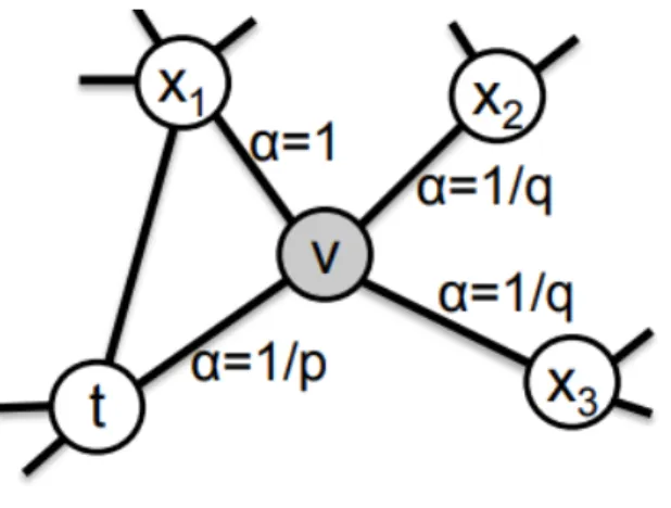
To solve this problem, second order random walks use 2 additional parameters which can be used to interpolate its behavior between DFS and BFS and control the revisit frequency of a given node. The first parameter is called the return parameter and is denoted by 𝑝. It governs how frequently we revisit a node in the walk. The second parameter is called as the InOut parameter. It is denoted by𝑞. It interpolates the behavior of the walk between DFS and BFS. If 𝑞 < 1, the walk behaves more like BFS. If 𝑞 > 1, the walk behaves more like DFS. These 2 parameters are used to generate a search bias, 𝛼, that is used to select the next node in the walk non-uniformly. The walk starts at a random node 𝑢, and it generates a sequence of nodes of length𝑙. Let’s say the walk was at node t and it selected node𝑣 as the next node and is currently at node 𝑣. There are 3 choices for the next node: 𝑥1, 𝑥2.𝑥3. The probability of choosing the next node, 𝑐𝑖, is given by the following equation:

𝑃(︀ 𝑐𝑖 =𝑥|𝑐𝑖−1 =𝑣 )︀ = ⎧ ⎪ ⎪ ⎨ ⎪ ⎪ ⎩ 𝜋𝑣𝑥/𝑍 𝑖𝑓(𝑣, 𝑥)∈𝐸 0 𝑜𝑡ℎ𝑒𝑟𝑤𝑖𝑠𝑒 where:

𝑍: normalizing constant

As mentioned earlier, there are problems with using the normalized edge weight as transition probability. So a search bias 𝛼 is used which is given by:

𝛼𝑝𝑞 = ⎧ ⎪ ⎪ ⎪ ⎪ ⎪ ⎪ ⎨ ⎪ ⎪ ⎪ ⎪ ⎪ ⎪ ⎩ 1/𝑝 𝑑𝑡𝑥 = 0 1 𝑑𝑡𝑥 = 1 1/𝑞 𝑑𝑡𝑥 = 2 where: t: node preceding 𝑣

Figure 6 shows how the search bias is computed using these 2 parameters using the above equation:

Figure 6: Search bias 𝛼 [1]

Algorithms 3 and 4 show the pseudocode for node2vec’s random walk and Skip-Gram procedures respectively.

Second order random walks facilitate exploration of diverse neighborhoods thereby learning rich representations of nodes.

Algorithm 3: Second order random walks

1 function randwalk2(G, 𝜋, 𝑙, 𝑢):

Input : 𝐺: Input Graph,

𝜋: Transition matrix,

𝑙: length of the walk,𝑢: starting node

Output: 𝑝𝑎𝑡ℎ: random walk

2 path = [u]

3 for i in range(l) do

4 v = path[-1] x = sample(neighbors(G, v)) append(path, x) 5 end

6 return path

Algorithm 4: node2vec Skip-Gram

1 function randwalk2(G, 𝑑, 𝑟, 𝑤, 𝑝,𝑞):

Input : 𝐺: Input Graph,

𝑑: Dimensions of vectors,

𝑟: walks per node, 𝑤: context size, 𝑝: inout parameter, 𝑞: return parameter

Output: 𝑋: vector representation of nodes

2 𝜋 = GenerateTransitionMatrix(G, p, q) 3 X = [] 4 walks = [] 5 for i in range(r) do 6 for node in G do 7 walks.append(randwalk2(G, 𝜋, l, u)) 8 end 9 end 10 X = GradientDescent(walks, w, d) 11 return X

Once the corpus is obtained, the algorithm uses Skip-Gram technique used by DeepWalk to obtain the embeddings. Similar to DeepWalk, different optimization techniques are used to reduce the computational complexity of the model. One of the most popular techniques is negative sampling [2]. In this technique, the input and output are modified slightly. Instead of the main word being the only input, the context word is also combined with the main word. The label is modified to indicate

Figure 7: node2vec Algorithm

whether the input pair is valid. So the label can simply be 0 and 1. Also, few random words are chosen from the dictionary for every main word for every bi-gram. These are called negative samples. The label for these samples is 0. Since the output layer only consists of a single node now, the model gets trained faster.

[1] emphasizes that it is possible to modify node2vec to obtain embeddings that preserve either structure or homophily or both. They demonstrate a case study using the Les Miserables [12] dataset which contains 77 nodes and 254 edges. The experi-ments generated 16-dimensional embeddings and clustering was performed using the k-means clustering algorithm.

In one of the experimental settings, the values of𝑝and𝑞were set to 1 and 0.5 re-spectively. The generated communities had characters that have frequent interactions with each other in the novel. Figure 9 shows the communities from this experiment. Another experiment had the values of 𝑝 and 𝑞 equal to 1 and 2 respectively. It gen-erated communities with nodes that structurally important in the network. Figure 8

Figure 8: Communities with structurally important nodes [1]

Figure 9: Homophilic communities [1]

shows the results of this experiment.

The datasets used for experimentation in [1] are BlogCatalog [13], protein-protein interactions (PPI) and Wikipedia word co-occurrence network. The results were evaluated on tasks like multilabel classification and link prediction [14]. The baseline algorithms used for performance evaluation are DeepWalk, Spectral Clustering, and LINE. Results show that node2vec was able to outperform the baseline algorithms.

However, the margins were not very huge. In some experiments, DeepWalk’s uniform exploration strategy performed just as good as the node2vec. However, the majority of the experiments show a substantial gain in the F1-score over baseline methods. This can be attributed to the added flexibility in the exploration of neighborhoods in node2vec.

It is evident that neighborhood exploration strategy plays the most important role in the quality of generated embeddings. Both DeepWalk and node2vec operate on the premise that searching local neighborhoods is enough for extracting relationships amongst nodes. However, the next section describes a method that relies on global statistics for information extraction.

3.3 Deep neural networks for learning graph representations (DNGR)

DNGR [15] argues that the information extraction methods used in the literature discussed so far is effective for unweighted graphs. These approaches rely on sampling the local structure of the graph. The size of the samples may also affect the generated embeddings depending on the available data. It also states that these methods are slow and perform unnecessary computations for capturing community information. Thus, DNGR explores different approaches other than sampling and answers the following 2 questions:

1. Is there a better way for capturing structural information more accurately for directed graphs?

2. Is there a better way of representing that information other than linear se-quences.

first and second order truncated random walks respectively. The length (𝑙) and total number of walks (𝜂) are hyperparameters. These techniques are very effective when the graph is unweighted because the connection of a node to its neighbors (topology) is the only information that is available for unweighted graphs. However, in the case of weighted and directed graphs, the edge weights influence the structural topology and can be used to extract more information. node2vec tries to solve this problem by biasing the search using 2 additional parameters for neighborhood exploration. This is effective and makes the random walk procedure flexible. However, their values are not easy to determine. Also, to capture enough statistical information, the number of random walks per node has to be large which makes the process slow. Further-more, these walks are eventually used to compute the co-occurrence matrix which can directly be calculated. So the computation of these walks is an overhead. Another problem with truncated random walks is that it is very difficult to capture correct contextual information of the nodes that are on the boundaries of the walk.

Due to these shortcomings, DNGR explores alternative approaches for learning representations based on matrix factorization techniques. These techniques have been empirically proven to outperform neural network based methods on certain tasks. One such method based on matrix factorization is hyperspace analogue analysis [16]. It uses the word-word co-occurrence matrix to obtain word-vector representations. But it has one problem. The words that occur very frequently with very little semantic meaning like stop words tend to have an adverse effect on the generated representa-tions. This problem is solved by using positive pointwise mutual information (PMI) matrix [17]. This matrix is a linear product of representation matrix and row vectors which can be factorized to obtain the representation matrix. The authors of [15] also point out that it is not necessary to use a linear model and hence DNGR uses a special

type of neural network called autoencoders [18].

DNGR model uses random surfer technique instead of random walks for ex-tracting the relationships amongst the nodes. This technique generates a node co-occurrence matrix. The matrix is a 𝑛*𝑛 square matrix and provides a global view of node statistics. The process begins with a transition matrix 𝐴. The values in the matrix represent the transition probability from node 𝑖 to node 𝑗. If a user is currently at node 𝑖, the probability that the user will jump to 𝑗 is the value given by 𝐴𝑖𝑗. This information is initially filled by using the edges given by the following

equation:

𝐴[𝑖][𝑗] = ∑︁

𝑖𝑗∈𝐸

𝑖𝑗/𝑑𝑒𝑔𝑟𝑒𝑒(𝑖)

Initially, the vertices are randomly ordered. Consider that the surfer is currently at𝑖𝑡_{ℎvertex. The model introduces a row vector𝑝}

𝑘for every vertex𝑖whose𝑗𝑡ℎentry

indicates the probability of reaching 𝑗𝑡_{ℎ vertex from 𝑖 after𝑘 surfing steps. Initially,} 𝑝𝑘 contains only 𝑖𝑡ℎ entry as one. The model also includes restarts where the surfer

could move to the next vertex with a probability𝛼or could start over from the initial vertex with a probability of1−𝛼. This model can be represented using the following equation:

𝑝𝑘=𝛼×𝑝𝑘−1×𝐴+ (1−𝛼)×𝑝0

It also takes the weight of context into account by introducing a monotonically decreasing weight function. This function has a lower value when the 𝑗𝑡ℎ node is far. The random surfing procedure is repeated for 𝑘 steps and an updated transition matrix is obtained. With this updated matrix, a PPMI matrix is computed with the help of the following equation:

Figure 10: DNGR [15]

where:

𝑃𝑖𝑗 =∑︀𝑛_𝑖=1∑︀𝑛_𝑗=1𝐴𝑖𝑗 𝑃𝑖 =∑︀𝑛_𝑖=1𝐴𝑖

𝑃𝑗 =∑︀𝑛_𝑗=1𝐴𝑗

A stacked denoising autoencoder (SDAE) [19] is used for learning the represen-tations. Autoencoders are special kind of neural networks which have a single hidden layer. The input data and the output label are the same. The network attempts to minimize reconstruction loss. The output from the hidden layer is used as the com-pressed representation. An SDAE contains multiple hidden layers and perturbs the input data with noise. This helps the network to learn more robust representations. Autoencoders have a lot of applications in the field of dimensionality reduction and data compression.

The PPMI matrix obtained is passed to an SDAE row-wise. Once the network is trained, the values generated by the hidden layer are the embeddings. Figure 10 shows the steps in the DNGR algorithm.

The experiments in [15] were performed using the 20-NewsGroup, Wikipedia Corpus and Wine datasets. The model’s performance was evaluated against Deep-Walk, SGNS, PPMI, and SVD as the baseline algorithms. The model outperformed

all the methods in the task of vertex clustering. In the task fo word-word similarity, its performance was as good as or better than most of the baselines. One interesting observation is that the quality of generated embeddings degrade if the value of 𝛼 is 1. If𝛼 approaches 1, the weight function has no effect on the contextual information. This emphasizes the importance of the weight function.

3.4 Core2Vec

Similar to DNGR, Core2Vec [20] also argues that the quality of generated random walks depends heavily on the topology and nature of the underlying graph. They suggest that the assumption that a random walk would always contain nodes that are semantically is fair in the case of assortative networks like social networks. However, for dissortative networks like biological networks, this need not be true. Dissortative networks have an interesting property called as core-periphery structure [21]. The core-periphery structure is formally defined as:

Let 𝐾 ⊆𝑉 be a set of vertices and𝐺(𝐾) be a subgraph induced on𝐾. 1. ∀𝑣 ∈𝐾, 𝑑𝐺(𝐾)(𝑣)>=𝑘,where 𝑑𝐺(𝐾)(𝑣) is the degree of𝑣 in 𝐺(𝐾) 2. ∀𝐾 ⊂𝐾′ ⊂𝑉, ∃𝑢∈𝐾′

𝐾𝑠𝑢𝑐ℎ𝑡ℎ𝑎𝑡𝑑𝐺(𝐾′_)(𝑢)<𝑘

If the above conditions hold true, then the𝐺is called as𝑘-core graph. 𝐾 is called the core set and𝑉 −𝐾 is called the periphery set. Simply stated, if a graph exhibits the core-periphery structure, the graph is partitioned into two sets 𝐾 and𝑉 −𝐾 and the subgraph formed by K is a dense subgraph. The nodes in the periphery set are adjacent to the nodes from the core set but not the other periphery nodes.

Figure 11: Core-periphery structure [21]

procedure which finds nodes from similar cores as candidates for walk progression. One interesting thing to note here is that this technique can effectively discover nodes in the same core as well as distant cores which should have semantic similarity based on the hypothesis that nodes in the similar cores play a similar role. Figure 11 shows an example of the core-periphery structure in a graph where nodes arranged in circles form the cores.

The authors exploit Skip-Gram model, similar to the previously discussed meth-ods. However, unlike these methods, the authors propose an objective function and optimize it using the stochastic gradient descent technique instead of using neural networks. The Skip-Gram model tries to maximize the likelihood probability of a context vector 𝐶𝑣𝑖 for a given vertex 𝑣. Thus, the objective function is given by:

𝑚𝑎𝑥𝑓 =∑︁ 𝑣∈𝑉 𝑃(𝐶𝑣|𝑣) = ∑︁ 𝑣𝑖𝑛𝑉 ∏︁ 𝐶_𝑣𝑖∈𝐶𝑣 𝑃(𝐶𝑣𝑖|𝑣)

Here, 𝑃(𝐶𝑣𝑖|𝑣) is the likelihood of seeing 𝑣𝑖 if a random walk is started from 𝑣 and is computed using:

𝑃(𝐶𝑣𝑖|𝑣) =𝑒𝑥𝑝(𝑣 𝑤_.𝐶𝑤 𝑣𝑖)/ ∑︁ 𝑣∈𝑉 𝑒𝑥𝑝(𝑣𝑤.𝐶_𝑣𝑤 𝑖)

where𝑣 and 𝑣𝑖 are main node and context node respectively, and 𝑣𝑤 and 𝐶𝑣𝑤𝑖 are their embeddings.

The proposed framework is very similar to the methods discussed previously. The first step generates random walks of fixed length and number. The experiments from the paper have these values set to 40 and 10. The second step computes the transition probabilities and initializes d-dimensional vectors for each node from a uniform distribution. The last step performs stochastic gradient descent on the ob-jective function using the generated walks. Algorithm 18 shows the pseudocode of the Core2Vec algorithm.

Algorithm 5: Core2Vec Algorithm

1 function core2vec(G, 𝑑,𝑟, 𝑤,𝑝, 𝑞):

Input : 𝐺: Input Graph,

𝑑: Dimensions of vectors,

𝑟: walks per node

Output: 𝑋: vector representation of nodes

2 k = 1 C = // Core mapping for nodes while |V| > 0 do

3 for v in |V| do 4 if deg(v) <= k then 5 del v; C[v] = k 6 else 7 continue 8 end 9 end 10 k = k + 1 11 end

12 walks = [] for i in range(r) do 13 walk = [] for j in range(l) do

14 curr = walk[-1] walk.append(Sample neighbors[curr])

15 end

16 walks.append(walk) 17 end

18 X = GradientDescent(G, walks, d) return X

metrics used for benchmarking are Closeness (𝐶) and Separability (𝑆). Closeness estimates how compact a given core is and Separability indicates how far are 2 dis-tinct cores. The experimental results from the paper show that core2vec obtains improvement over DeepWalk and LINE which in some cases is as high as 46%.

Core2Vec successfully demonstrates the idea of utilizing global information like core-structure of a network to extract semantic relationships amongst nodes and sup-ports the intuition of GloVe to utilize global statistics of a network to derive semantic relationships.

CHAPTER 4

GloVeNoR for node embeddings

4.1 Background

GloVe [3] was originally developed in 2014 for computing vector representations of words as a part of Stanford NLP research. GloVe is a global, unsupervised log bilinear regression model that takes into account both, the local context window similarity and global context similarity for computing the embeddings. The intuition behind GloVe is very simple: Global word-word co-occurrence statistics can potentially reveal information about word similarities. As a result, GloVe word embeddings excel at tasks like finding words with similar meaning (nearest neighbors). This is ideal for community detection problems as communities can be viewed as a collection of nodes which are semantically similar to each other.

4.2 GloVe for word embeddings

The authors of GloVe [3] mention that techniques like skip-gram and context window used in word2vec have a disadvantage of not learning from global statistics. Core2Vec[21] also supports this hypothesis and uses the global core-periphery struc-ture to find similar nodes. As a result, word repetitions and bigger patterns might not be learned with these methods. The way GloVe tackles this problem is by building a word-word co-occurrence matrix. The Algorithm then maximizes the probability of given context word appearing within a window of another word called as the main or center word.

The objective of the model is a simple weighted least squares function. The model also uses a weight function to deal with outliers and co-occurrences that are

seen very rarely. Algorithm 6 describes the steps of GloVe algorithm.

Algorithm 6: GloVe algorithm for word embedding

1 function GloVe(C, w):

Input : 𝐶: text corpus,

𝑤: context window length,

𝑑: vector dimensions

Output: 𝑉: word vectors

2 voc = buildVocab(C); 3 M = buildCooccur(C, voc); 4 V = initRandomVectors(d) 5 trainModel(M, V)

6 return V;

The cost function for the model is given as:

𝐽 = 𝑉 ∑︁ 𝑖,𝑗=1 𝑓(︀𝑋𝑖𝑗) (︀ 𝑤𝑇_𝑖 ·𝑤˜𝑗 +𝑏𝑖+ ˜𝑏𝑗 −𝑙𝑜𝑔𝑋𝑖𝑗)2 where: i = main word j = context word

𝑤𝑖 = main word vector

𝑤𝑗 = context word vector

X = co-occurrence matrix

𝑏𝑖, 𝑏𝑗 = bias vectors

V = vocabulary size

The weight function that was empirically found to be effective is given as: 𝑓(︀ 𝑋𝑖𝑗 )︀ = ⎧ ⎪ ⎪ ⎨ ⎪ ⎪ ⎩ (𝑥/𝑥𝑚𝑎𝑥)𝛼 𝑥 < 𝑥𝑚𝑎𝑥 1 𝑜𝑡ℎ𝑒𝑟𝑤𝑖𝑠𝑒

4.3 Proposed Algorithm - GloVeNoR

In our approach, we decided to use second order random walks from [1] because of the flexibility they provide for neighborhood exploration. We wanted the sampling behavior of the random walks to be approximated between DFS and BFS so the value of 𝑝and 𝑞 were set to 1. Algorithm 7 provides an outline of the proposed GloVeNoR model. The procedure on line 2 iterates over all the nodes of the input graph 𝐺 and generates 𝑘 random walks of length 𝑙 per node.

Algorithm 7: GloVeNoR for Graphs

1 function GloVeNoR(G, w, d, l, k, p, q, i):

Input : 𝐺: input graph,

𝑤: context window length,

𝑑: vector dimensions,

𝑙: length of random walks

𝑘: number of walks per node,

𝑝: inout parameter,

𝑞 return parameter,

𝑖: number of training iterations

Output: 𝑉: node vectors

2 corpus = generate2RandomWalks(G, k, p, q, l) 3 M = buildCooccur(corpus, w);

4 V = initRandomVectors(d) 5 trainModel(M, V, i return V;

The generated corpus is used by the co-occurrence matrix generator procedure on line 3. The co-occurrence matrix generator is the gist of the GloVeNoR model. In contrast to [1] and [15], it captures the global co-occurrence statistics for all the

nodes. For every node, 𝑖, in a walk, the procedure iterates over all the nodes, 𝑗, in a window of size 𝑤 from 𝑖, and updates the [𝑖, 𝑗]𝑡ℎ _{entry of 𝑀 with the reciprocal}

of distance between 𝑖 and 𝑗. Intuitively, the value for a pair of nodes 𝑖 and 𝑗 in

𝑀 is higher for the nodes co-occurring frequently in the corpus. The output of this procedure is a |𝑉| × |𝑉| matrix 𝑀, where|𝑉| is the number of nodes.

In the next step, vectors of dimension 𝑑 are initialized by the procedure on line 5. These vectors are initialized from a random distribution and optimized to obtain the final embeddings. The procedure on line 4 implements the objective function given in section 4.2 and optimizes it using Gradient Descent for 𝑖 iterations. This step generates the final node embedding matrix𝑉. The size of 𝑉 is|𝑉| ×𝑑and every row of 𝑉 represents a vector corresponding to a node in the graph.

4.4 An example of GloVeNoR

This section illustrates a sample execution of the algorithm on an example graph. In Figure 12 we have a random Erdős-Renyi graph with𝑝= 1/2. It is an unweighted, undirected graph with 10 nodes and 30 edges. The first step of the algorithm takes this graph as input and generates the random walks corpus. We used the values for number of walks per node,𝑘 = 1 and length of a walk,𝑙 = 5. The output of this step is as follows: 0,8,2,3,5 1,7,4,2,3 2,3,5,9,8 3,0,8,1,7 4,0,7,1,0

Figure 12: A sample Erdős-Renyi graph with 10 nodes and 30 edges 5,3,2,4,7 6,8,0,3,4 7,0,8,3,4 8,3,0,1,6 9,5,2,4,7

The next step generates the co-occurrence matrix using this corpus. We used a window size𝑤= 1 for the above corpus. The generated co-occurrence matrix is given by: 0.0 2.0 0.0 3.0 1.0 0.0 0.0 2.0 4.0 0.0 2.0 0.0 0.0 0.0 0.0 0.0 1.0 3.0 1.0 0.0 0.0 0.0 0.0 4.0 3.0 1.0 0.0 0.0 1.0 0.0 3.0 0.0 4.0 0.0 2.0 3.0 0.0 0.0 2.0 0.0 1.0 0.0 3.0 2.0 0.0 0.0 0.0 3.0 0.0 0.0 0.0 0.0 1.0 3.0 0.0 0.0 0.0 0.0 0.0 2.0 0.0 1.0 0.0 0.0 0.0 0.0 0.0 0.0 1.0 0.0 2.0 3.0 0.0 0.0 3.0 0.0 0.0 0.0 0.0 0.0 4.0 1.0 1.0 2.0 0.0 0.0 1.0 0.0 0.0 1.0 0.0 0.0 0.0 0.0 0.0 2.0 0.0 0.0 1.0 0.0

Figure 13: Generated communities

initialized for every node. These vectors are optimized in the final step using the co-occurrence matrix and the cost function given in section 4.2 The final step trains the GloVeNoR model using the co-occurrence matrix. This step generates𝑑-dimensional embeddings of the graph nodes. For the above example, the dimensionality,𝑑, of the embeddings is 2. The generated vectors are given by:

0.00032430148178421857 0.7938853234927894 0.47120730004410316 0.07747351511500729 0.6995203607385199 0.22675897204604747 0.40398774088300593 0.3402914202062996 0.3684166382730359 −0.0466443816755288 −0.09899558914305986 0.3546439090539501 0.32795573825915464 0.32323114306831036 0.3240960932604696 0.21676116252743483 −0.15893379881151024 0.7265621806582748 0.30177281552368374 0.3173293382685133

These vectors are clustered using the k-means clustering algorithm. The gener-ated clusters are communities in the graph. In the above example, we are using a k value of 2. The generated communities are shown in Figure 13.

CHAPTER 5

Implementation and Experiments

This chapter elaborates on the experiments performed on different real-world data sets. It is organized into 6 different sections. The first section elaborates on the implementation details. Further sections describe a dataset and experimental results obtained on that dataset and some visualizations. The experiments primarily focus on 3 different hyper-parameters, the length of random walks, context window and vector dimensionality. Since we do not have any ground truth, we would be using silhouette score and modularity as our comparison metric.

5.1 Implementation Details

The project is implemented as a collection of Python modules. The list of mod-ules is given below. The programming language of choice is Python. The reason for choosing Python is the availability of a large number of machine learning and graph processing libraries. We are using igraph and networkx for reading and performing operations on graph files. We are using numpy for computing co-occurrence matrix. We are also using library implementations of DeepWalk and node2vec. Following list summarizes the implemented modules:

1. The first module takes a graph file in GML format as input and generates a CSV file containing random walks as the output. A random walk is a sequence of comma-separated node ids from the graph.

2. The second module takes this corpus of random walks as inputs, parsed it and generates an n * n cooccurrence matrix. This matrix is written to a file in space

Figure 14: GloVeNoR Phases

separated format.

3. The third module implements the GloVeNoR model. It takes the co-occurrence file as input, trains the GloVeNoR model using Stochastic Gradient Descent and creates an output file which contains the vectors for graph nodes.

4. There are also utility scripts which perform the clustering operation on these vectors and compute node2vec embeddings for evaluation.

Figure 14 shows the various steps involved in the algorithm. Figure 15 shows the workflow used for performing experiments which are discussed in the following section in greater detail. Figure 16 shows the use of generated embeddings for finding communities in the graph.

5.2 Zachary’s Karate Club dataset

Zachary’s Karate Club dataset [22] is a famous network dataset curated by Wayne W. Zachary. This dataset has 34 nodes representing 34 people. There is an edge between two people if they interact socially outside the club. There are 78 edges. The diameter of this network is 5. Figure 17 shows a visualization of this dataset.

An interesting fact about this data set is that there was a conflict between the instructor and the administrator which led them starting their own clubs. Thus the nodes were split into 2 clubs. As mentioned earlier, the primary hyperparameters

Figure 15: GloVeNoR Workflow

that would be considered in the experiments are window size, dimensionality and walk length.

Tables 1, 2, 3 summarize the observations for different values of the hyperparam-eters. We used K-means clustering to generate the communities from the embeddings. The k value was varied from 2 to 8 in the steps of 2 and observations were recorded. The above values are the maximum values from these experiments. It can be clearly seen that GloVeNoR has better modularity values of all the three. In some cases,

Figure 16: GloVeNoR Applications

Figure 17: Zachary’s Karate Club dataset

GloVeNoR lags behind in the silhouette score. However, since our primary target is to community detection, a good modularity score is desirable. An interesting obser-vation from Table 3 is that modularity value tends to stabilize around window size 4 and 5. The diameter of the graph is 5 as well. Thus intuitively, we can use this as a result for further experiments. Also, the maximum modularity value achieved for the Zachary’s Karate Club dataset is 0.4197. This value was achieved when the number

Table 1: Zachary’s Karate Club dataset: Comparison of results for different walk lengths

Walk lenth GloVeNoR

(Silhouette score, modularity) DeepWalk (Silhouette score, modularity) node2vec (Silhouette score, modularity) 10 0.3940,0.4197 0.3947, 0.2287 0.3859, 0.2043 15 0.4300,0.4197 0.5891, 0.0200 0.3935, 0.2043 20 0.4189,0.4197 0.6301, -0.0210 0.4105, 0.2043 25 0.4325,0.4197 0.5849, -0.0293 0.4106, 0.2043 30 0.4098,0.4197 0.5375, -0.0670 0.4117, 0.1674

Table 2: Zachary’s Karate Club dataset: Comparison of results for different vector dimensions Vector Di-mensions GloVeNoR (Silhouette score, modularity) DeepWalk (Silhouette score, modularity) node2vec (Silhouette score, modularity) 2 0.5720,0.3600 0.6715, -0.0670 0.6980, 0.1634 4 0.5475,0.4197 0.5662, -0.0891 0.5949, 0.1674 6 0.4180,0.4197 0.5353, -0.1180 0.4664, 0.1674 8 0.4135,0.4197 0.5500, -0.0670 0.4363, 0.1674 10 0.4272,0.4197 0.5500, -0.0670 0.4174, 0.1674

of communities was equal to 4. Another interesting observation from the experiments is that the model tends to find the local minimum quickly if the size of the context window is closer to or greater than the diameter of the graph. Thus, we can conclude that GloVeNoR discovered 4 communities in the Zachary’s Karate Club graph. The information in the tables is graphically shown in the following visualizations.

The observations about the hyperparameters from the Zachary’s Karate Club dataset can be used as the basis for experimentation on the further datasets.

Table 3: Zachary’s Karate Club dataset: Comparison of results for different context window sizes Window size GloVeNoR (Silhouette score, modularity) DeepWalk (Silhouette score, modularity) node2vec (Silhouette score, modularity) 1 0.1932,0.2068 0.5446, -0.0502 0.4129, 0.1674 2 0.3616,0.3980 0.5717, -0.0502 0.4181, 0.2043 3 0.4116,0.4197 0.5500, -0.0502 0.4067, 0.1655 4 0.4077,0.4197 0.5440, -0.0502 0.4048, 0.1674 5 0.3986,0.4197 0.5363, -0.0670 0.3939, 0.2043 6 0.4307,0.4197 0.5416, -0.0545 0.3856, 0.2043 7 0.4392,0.4197 0.5418, -0.0545 0.3821, 0.1674 8 0.4528,0.4197 0.5225, -0.0502 0.3821, 0.1674 9 0.4398,0.4197 0.5225, -0.0502 0.3821, 0.1643 10 0.4516,0.4197 0.4829, -0.0670 0.3776, 0.1674

Table 4: Harry Potter dataset: Comparison of results for different walk lengths Walk lenth GloVeNoR

(Silhouette score, modularity) DeepWalk (Silhouette score, modularity) node2vec (Silhouette score, modularity) 10 0.3940,0.2039 0.3941, 0.0022 0.1825, 0.0012 15 0.2339,0.2085 0.3886, 0.0071 0.2956, 0.0024 20 0.2249,0.1910 0.3972, 0.0022 0.3016, 0.0095 25 0.2249,0.2125 0.3886, 0.0053 0.3059, 0.0047 30 0.2242,0.2114 0.3941, 0.0022 0.3102, 0.00431

5.3 Harry Potter Dataset

The Harry Potter dataset [23] contains 178 nodes and 2453 edges. Each node represents a character in the Harry Potter universe. Two nodes have an edge between them if they have some logical connection to each other in the books. The diameter of the network is 3. Tables summarize experimental results.

Tables 4, 5, 6 summarize the experiments performed on the Harry Potter dataset. We ran the k-means clustering on the dataset and recorded the above values. The

Figure 18: Walk length vs Modularity and Silhouette score

value of k was varied from2to20. It can be observed that the results are in agreement with the experiments performed on the Zachary’s Karate Club dataset. GloVeNoR has the best modularity score of all the three methods. The length of walks does not have a significant effect on the modularity. The modularity value stabilizes to a good value when the window size is close to the diameter of the graph. The silhouette score values generated by GloVeNoR are comparable to the ones produced by node2vec. However, DeepWalk has the best silhouette score.

Figure 19: Number of communities vs Modularity and silhouette score

5.4 Facebook Dataset

The Facebook dataset [24] contains 4039 nodes and 88,234 edges. A node in this dataset represents a Facebook user and an edge joins two users that are friends on Facebook. This dataset was collected by surveying users using an application on Facebook. All the user information is randomized, replaced and anonymized to protect the privacy of the participants. The diameter of the network is 8. We use the observations from our previous experiments and keep window size for co-occurrence

Figure 20: Vector dimension vs Modularity and Silhouette score

matrix generation equal to 8 which is equal to the diameter of the network. We also keep the walk length to 10 which is slightly greater than the diameter and should be enough to cover the farthest vertices of the graph. We set the window size to 8. The dimension of the embeddings was set to 10. The number of random walks per node was 385. Same values were used for all the three methods while performing experiments. Table 7 summarizes the observations. GloVeNoR outperforms all the other methods in the modularity score by a significant margin. The silhouette score

Figure 21: Context window vs Modularity and Silhouette score

value for GloVeNoR is comparable to node2vec but lags far behind that of DeepWalk.

5.5 Wikivote dataset

The Wikivote dataset [25] contains7115nodes and100,762edges. The diameter of the network is7. Wikipedia conducts elections to promote a user to administrator status. A node in this network represents a wikipedia user and an edge between node

Table 5: Harry Potter dataset: Comparison of results for different vector dimensions Vector Di-mensions GloVeNoR (Silhouette score, modularity) DeepWalk (Silhouette score, modularity) node2vec (Silhouette score, modularity) 2 0.4997,0.2033 0.5986, 0.0029 0.5325, 0.0121 4 0.4223,0.2018 0.5986, 0.00574 0.466, 0.0047 6 0.3653,0.2109 0.4967, 0.0071 0.3797, 0.0097 8 0.3007,0.2069 0.4319, 0.0096 0.3285, 0.0016 10 0.2626,0.2045 0.3951, 0.0051 0.309, 0.0036

Table 6: Harry Potter dataset: Comparison of results for different context window sizes Window size GloVeNoR (Silhouette score, modularity) DeepWalk (Silhouette score, modularity) node2vec (Silhouette score, modularity) 1 0.0899,0.0021 0.2040, 0.0020 0.2068, 0.0039 2 0.2174,0.1969 0.3582, 0.0024 0.2045, 0.0049 3 0.212, 0.2137 0.3686, 0.0008 0.283, 0.0109 4 0.2531,0.2083 0.3830, 0.0025 0.2996, 0.0013 5 0.2630,0.2137 0.3953, 0.0037 0.3089, 0.0037

wikipedia voting data until the year 2008. Similar to the Facebook dataset, we kept the hyperparameter values close to our observations from the previous results. The length of the walks is 8. The window size is 7. The dimensionality of the vectors is 10. The number of random walks per node is218.

Table 8 summarizes the results of our experiments. The results are consistent Table 7: Facebook dataset: Comparison of the methods

GloVeNoR (Silhouette score, modularity) DeepWalk (Silhouette score, modularity) node2vec (Silhouette score, modularity) 0.1945,0.665 0.5716, 0.2785 0.2725, 0.3297

Table 8: Wikivote dataset: Comparison of the methods GloVeNoR (Silhouette score, modularity) DeepWalk (Silhouette score, modularity) node2vec (Silhouette score, modularity) 0.1005,0.3585 0.8164, 0.0011 0.759, 0.0015

Table 9: Astro dataset: Comparison of the methods GloVeNoR (Silhouette score, modularity) DeepWalk (Silhouette score, modularity) node2vec (Silhouette score, modularity) 0.0953,0.5320 0.7488, 0.0134 0.1662, 0.4825

with our previous experiments. GloVeNoR produces the best modularity scores of all. However, one difference here is that the silhouette score for GloVeNoR is much lower than that of DeepWalk and node2vec.

5.6 Astro dataset

The Astro dataset [26] is a co-authorship network of papers published on the topic of astrophysics from ArXiv. A node represents an author. There is an undirected edge between 2 nodes,𝑖and𝑗, if they have co-authored a paper. The dataset contains 18,772 nodes and 198,110 edges. The diameter of the network is 14. The length of the walks we used is 30. The window size is equal to 14 and the dimensionality of the embeddings is 10. The number of random walks per node is 12.

Observations from Table 9 are in agreement with the results from previous datasets. GloVeNoR consistently produces better modularity values and DeepWalk has the best silhouette score.

CHAPTER 6

Conclusion and future work

6.1 Conclusion

We successfully achieved the objective of this project to port the GloVeNoR model to generate node embeddings for graphs. We evaluated the quality of gen-erated embeddings on the task of community detection. We extensively researched existing work in this domain and found some state-of-the-art node embedding models like node2vec, DeepWalk, DNGR, and Core2Vec. We reused some ideas from these techniques like second order random walks for this project. We compared the perfor-mance of our model against node2vec and DeepWalk by using metrics like silhouette score and modularity.

We conducted experiments on 5 network datasets. We found out that GloVeNoR consistently produced better modularity scores than node2vec and DeepWalk on all the datasets. GloVeNoR produced similar silhouette scores as that of node2vec but DeepWalk produced the best silhouette scores of all. We targeted three hyperparam-eters in our experiments: length of walks, dimensionality of embeddings and window size. We observed that the length of walks did not have a substantial effect on the modularity and silhouette scores if the value is close to or greater than the diameter of the graph. We also observed that the modularity value stabilized if the window size is equal to or greater than the diameter. Another interesting observation is that the GloVeNoR model trained quickly for higher dimensions.

6.2 Future Work

The possible directions for future work on this project are to explore the impact of other hyperparameters like the return parameter (𝑝) and in-out parameter (𝑞) used in the generation of random walks. The algorithm can also be tested on different tasks like link prediction and graph classification. Lastly, methods other than random walks can be explored to extract node information from a graph.

LIST OF REFERENCES

[1] A. Grover and J. Leskovec, “Node2vec: Scalable feature learning for networks,” in

Proceedings of the 22Nd ACM SIGKDD International Conference on Knowledge

Discovery and Data Mining, KDD ’16, (New York, NY, USA), pp. 855–864,

ACM, 2016.

[2] T. Mikolov, K. Chen, G. Corrado, and J. Dean, “Efficient estimation of word representations in vector space,” in 1st International Conference on Learning Representations, ICLR 2013, Scottsdale, Arizona, USA, May 2-4, 2013,

Work-shop Track Proceedings, 2013.

[3] J. Pennington, R. Socher, and C. D. Manning, “Glove: Global vectors for word representation,” in Empirical Methods in Natural Language Processing

(EMNLP), pp. 1532–1543, 2014.

[4] L. Vilnis and A. McCallum, “Word representations via gaussian embedding,”

in 3rd International Conference on Learning Representations, ICLR 2015, San

Diego, CA, USA, May 7-9, 2015, Conference Track Proceedings, 2015.

[5] M. E. J. Newman, “Modularity and community structure in networks,”

Proceed-ings of the National Academy of Sciences, vol. 103, no. 23, pp. 8577–8582, 2006.

[6] M. E. J. Newman and M. Girvan, “Finding and evaluating community structure in networks,” Phys. Rev. E, vol. 69, p. 026113, Feb 2004.

[7] B. Perozzi, R. Al-Rfou, and S. Skiena, “Deepwalk: Online learning of social repre-sentations,” in Proceedings of the 20th ACM SIGKDD International Conference

on Knowledge Discovery and Data Mining, KDD ’14, (New York, NY, USA),

pp. 701–710, ACM, 2014.

[8] C. Avin and B. Krishnamachari, “The power of choice in random walks: An empirical study,” in Proceedings of the 9th ACM International Symposium on

Modeling Analysis and Simulation of Wireless and Mobile Systems, MSWiM ’06,

(New York, NY, USA), pp. 219–228, ACM, 2006.

[9] J. yu Pan, H. Yang, P. Duygulu, and C. Faloutsos, “Automatic multimedia cross-modal correlation discovery,” in In KDD, pp. 653–658, 2004.

[11] F. Morin and Y. Bengio, “Hierarchical probabilistic neural network language model,” in Proceedings of the Tenth International Workshop on Artificial

Intel-ligence and Statistics (R. G. Cowell and Z. Ghahramani, eds.), pp. 246–252,

Society for Artificial Intelligence and Statistics, 2005.

[12] D. E. Knuth, The Stanford GraphBase: A Platform for Combinatorial Comput-ing. New York, NY, USA: ACM, 1993.

[13] R. Zafarani and H. Liu, “Social computing data repository at ASU,” 2009. [14] L. Backstrom and J. Leskovec, “Supervised random walks: Predicting and

rec-ommending links in social networks,” CoRR, vol. abs/1011.4071, 2010.

[15] S. Cao, W. Lu, and Q. Xu, “Deep neural networks for learning graph representa-tions,” inProceedings of the Thirtieth AAAI Conference on Artificial Intelligence, AAAI’16, pp. 1145–1152, AAAI Press, 2016.

[16] K. Lund and C. Burgess, “Producing high-dimensional semantic spaces from lexical co-occurrence,” Behavior Research Methods, Instruments, & Computers, vol. 28, pp. 203–208, Jun 1996.

[17] K. W. Church and P. Hanks, “Word association norms, mutual information, and lexicography,” Comput. Linguist., vol. 16, pp. 22–29, Mar. 1990.

[18] H. Bourlard and Y. Kamp, “Auto-association by multilayer perceptrons and sin-gular value decomposition,” Biol. Cybern., vol. 59, pp. 291–294, Sept. 1988. [19] P. Vincent, H. Larochelle, I. Lajoie, Y. Bengio, and P.-A. Manzagol, “Stacked

denoising autoencoders: Learning useful representations in a deep network with a local denoising criterion,” J. Mach. Learn. Res., vol. 11, pp. 3371–3408, Dec. 2010.

[20] S. Sarkar, A. Bhagwat, and A. Mukherjee, “Core2vec: A core-preserving feature learning framework for networks,” in IEEE/ACM 2018 International Confer-ence on Advances in Social Networks Analysis and Mining, ASONAM 2018,

Barcelona, Spain, August 28-31, 2018, pp. 487–490, 2018.

[21] M. Rombach, M. Porter, J. Fowler, and P. Mucha, “Core-periphery structure in networks,” SIAM Journal on Applied Mathematics, vol. 74, no. 1, pp. 167–190, 2014.

[22] R. A. Rossi and N. K. Ahmed, “The network data repository with interactive graph analytics and visualization,” in Proceedings of the Twenty-Ninth AAAI

Conference on Artificial Intelligence, 2015.

[24] J. Leskovec and J. J. Mcauley, “Learning to discover social circles in ego net-works,” in Advances in Neural Information Processing Systems 25 (F. Pereira, C. J. C. Burges, L. Bottou, and K. Q. Weinberger, eds.), pp. 539–547, Curran Associates, Inc., 2012.

[25] J. Leskovec, D. Huttenlocher, and J. Kleinberg, “Signed networks in social me-dia,” in Proceedings of the SIGCHI Conference on Human Factors in Computing

Systems, CHI ’10, (New York, NY, USA), pp. 1361–1370, ACM, 2010.

[26] J. Leskovec, J. Kleinberg, and C. Faloutsos, “Graph evolution: Densification and shrinking diameters,” ACM Trans. Knowl. Discov. Data, vol. 1, Mar. 2007.