Improving Classification of Very-High-Resolution Satellite Imagery - Combining Invariant Support Vector Machines and Object-Based Image Analysis to Tackle Limited Information Input

H

U

F

C

E

S

I

G

Bachelor´s Thesis

Improving Classification of Very-High-Resolution

Satellite Imagery

Combining Invariant Support Vector Machines and Object-Based Image Analysis to

Tackle Limited Information Input

February 14th, 2017

A

:

R

:

ii

EIDESSTATTLICHE ERKLÄRUNG

Ich erkläre hiermit, dass ich diese Bachelorarbeit selbstständig, ohne die Hilfe Dritter und ohne die Nutzung anderer Quellen und Hilfsmittel als angegebenen, verfasst habe. Alle den genutzten Quellen wörtlich oder sinngemäß entnommenen Stellen, sind als solche einzeln kenntlich gemacht. Gleiches gilt auch für beigegebene Abbildungen und Kartenskizzen. Diese Arbeit ist bislang keiner anderen Prüfungsbehörde vorgelegt worden und auch nicht veröffentlicht worden.

iii

ABSTRACT

Addressing environmental and socioeconomic challenges in the context of climate change or urbanization, often requires monitoring of large spatial areas. As remote sensing can provide such information, it evolved to be a standard tool to work on related subjects. Image classification often forms the basis for used workflows and derived products. The emergence of new sensor technologies which provide very high spatial and spectral resolution data, made the consideration of objects at finer scales possible and broadened the scope of potential applications of remote sensing. Novel image processing and classification methods such as object-based image analysis and support vector machines, are introduced to effectively exploit the information provided by improved resolutions. Nevertheless, especially for supervised approaches, classification results still depend strongly on the amount and distribution of available ground truth data as information input for training of classifiers. This thesis aims to address the issue by proposing a generic method capable of coping with small ground truth data sets to classify very high spatial resolution data. This is done by transferring invariant support vector machines to the methodology of object-based image analysis. Resulting classifiers appear invariant to scale or geometry representation in ground truth data sets and thus achieve better classification accuracies on limited information input. Experiments on a very-high-resolution image of a complex urban land cover composition – cologne city center – suggest that the proposed method has much scope for future developments. Results show 0.2-0.03 points of 𝜅 accuracy improvement (to reach 0.57-0.79) on small ground truth data sets (20 or less training samples per class) compared to a state of the art classification system for a binary classification problem. Although less pronounced, multi-class settings resemble those tendencies. However, in order to ensure general validity of the results, further research is needed.

iv

ZUSAMMENFASSUNG

Aktuelle Umweltprobleme und sozioökonomische Herausforderungen, wie sie im Kontext von Klimawandel oder Urbanisierung auftreten, erfordern häufig die Beobachtung und Untersuchung großflächiger Gebiete. Die Fernerkundung hat sich in diesem Zusammenhang als effiziente Methode bewährt, deren Ergebnisse maßgeblich auf Bildklassifizierungen aufbauen. Durch technische Weiterentwicklungen werden immer höhere räumliche und spektrale Auflösungen erzielt. Gleichzeitig etablieren sich neue Methoden der Bildverarbeitung und Klassifizierung, darunter objektbasierte Verfahren und Support Vector Machines, die den Informationsgehalt hoher Auflösungen nutzbar machen sollen. Dennoch hängen Klassifikationsergebnisse, insbesondere für überwachten Klassifikationsmethoden, stark von verfügbaren Trainingsgebieten und in-situ Daten ab, da diese Referenzdatensätze für das Ableiten von Entscheidungsfunktion des Klassifikators nötig sind. Diese Arbeit stellt eine Methode vor, die auf das Klassifizieren von räumlich hochaufgelösten Satellitenbildern anhand von minimal verfügbaren Testgebieten ausrichtet ist. Objektbasierte Klassifizierung wird dafür mit der Virtual Support Vector Machine in einen Arbeitsablauf integriert. Erzeugte Klassifikatoren werden dadurch invariant zu spezifischen Größen- oder Geometrieeigenschaften von Bildobjekten aus verfügbaren Trainingsgebieten. Dadurch verbessert sich vor allem für Situationen mit limitierter Verfügbarkeit von Testflächen die Qualität des Klassifikationsergebnisses. Die an einer räumlich hochaufgelösten Szene des Stadtzentrums von Köln durchgeführten Experimente liefern vielversprechende Ergebnisse. Verglichen mit einem objektbasierten State-of-the-Art-Klassifikator können für Situationen mit wenigen verwendeten Testgebieten (20 oder weniger Samples pro Klasse) Verbesserungen zwischen 0.2-0.03 Punkte 𝜅 Genauigkeit (auf insgesamt 0.57-0.79) eines binären Klassifikationsergebnisses erzielt werden. Diese Tendenzen bestätigen sich auch unter Einbezug mehrerer Klassen, wenn auch weniger ausgeprägt. Um jedoch zu allgemeingültigen Ergebnissen zu kommen, sind weitere Experimente erforderlich.

v

ACKNOWLEDGEMENTS

I would like to thank Dr. Susanne Schmidt for her support and supervision on this work which includes thematic supervision during the working process but also the provision of a workspace for long-lasting computer calculations at the South Asian Institute of Heidelberg University. I would like to thank Dr. Christian Geiß for his constant availability for professional advice and willingness to discuss challenges that emerged along the way. My gratitude also goes to Patrick Manuel Aravena Pelizari. Thank you both for giving me the opportunity to work on your idea of combining OBIA and VSVM, during my internship and as basis of this thesis. Also, thank you and the entire DLR team “Modelling and Geostatistical Methods”, at the Department of Geo-Risks and Civil Security, for providing satellite data of Cologne as well as the corresponding ground truth data set.

vi

CONTENT

Figures ... vii

Abbreviations ... viii

Symbols Used for Models and Model Components ... ix

1 Introduction ... 1

2 Object-Based Image Analysis ... 4

Image Segmentation ... 5

Image-Object Features ... 7

2.2.1 Spectral ... 7

2.2.2 Texture ... 8

2.2.3 Shape ... 9

3 Support Vector Machine Classification ...10

Theoretical Background ...10

SVMs in Remote Sensing...13

Invariances in SVMs ...14

4 Invariances in supervised Object Based Classification ...16

Invariance in Scale and Geometry ...16

Proposed Methodology ...17

4.2.1 Ground Truth Data Sets ...17

4.2.2 Segmentation Procedure ...18

4.2.3 Basis SVM Classification ...19

4.2.4 VSV Generation and Integration ...20

4.2.5 Optimization Procedure ...21

4.2.5.1 Measure of Feature Similarity ...21

4.2.5.2 Adapted Margin Sampling Strategy ...23

4.2.6 Final Model ...23

5 Experiments ...24

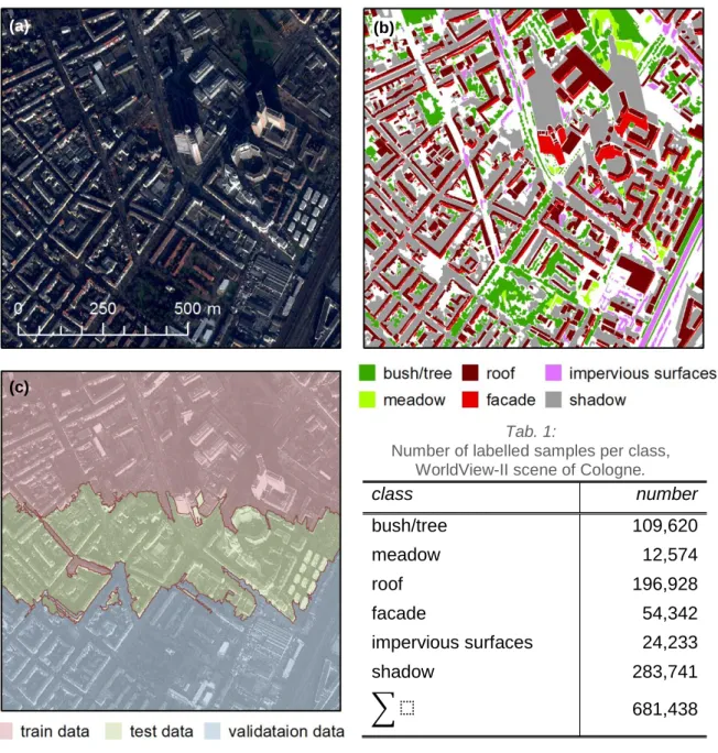
WorldView-II Scene of Cologne, Germany ...24

Experimental Setup ...26

6 Results ...28

Scale Invariance ...28

Geometry Invariance ...29

7 Discussion ...31

8 Conclusion and Outlook ...33

Source of Satellite Data ...35

vii

FIGURES

Fig. 1: Relationship of ground sampling distance with object of interest. ... 2

Fig. 2: Image segments in relation with objects of interest. ... 4

Fig. 3: Concept of Multiresolution Image Segmentation. ... 6

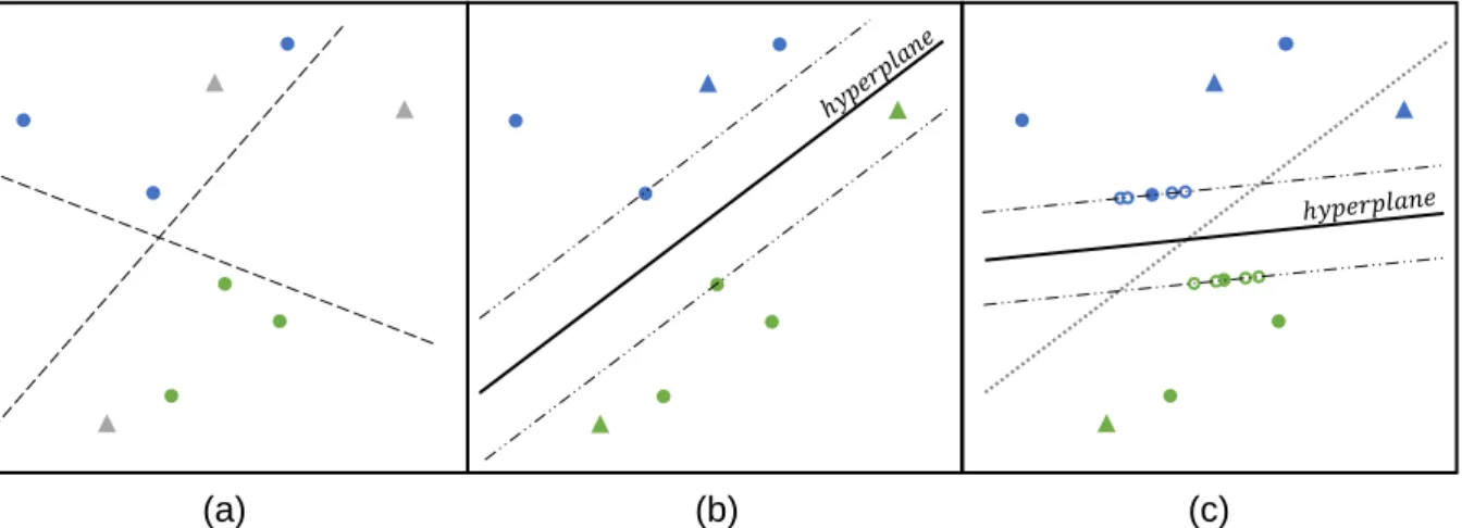
Fig. 4: Idealized process of locating the optimal separating hyperplane. ... 10

Fig. 5: Idealized process of defining a nonlinear decision function by SVMs. ... 11

Fig. 6: Simplified functionality of VSVMs... 15

Fig. 7: Block scheme of the proposed method. ... 17

Fig. 8: Exemplary generation of VSVs. ... 20

Fig. 9: Principle functionality of the optimization procedure for potential VSVs. ... 22

Fig. 10: Data foundation, WorldView-II scene of Cologne, Germany. ... 25

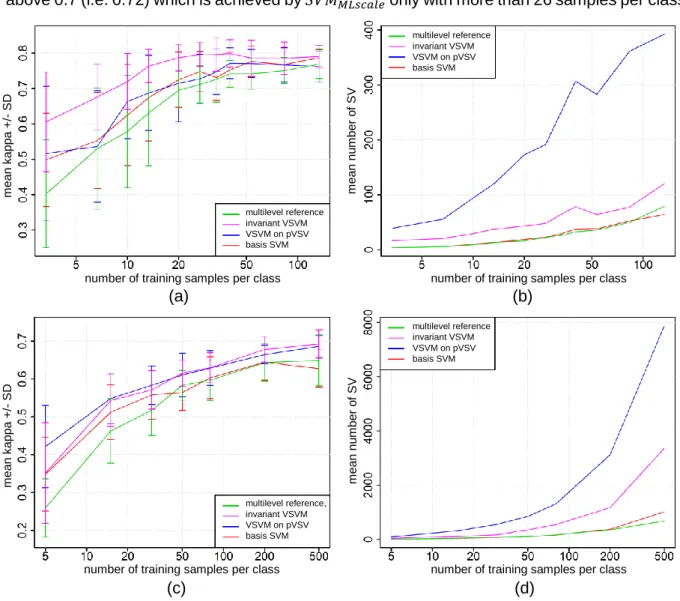
Fig. 11: Classification results for experiments considering scale invariance. ... 28

viii

ABBREVIATIONS

VHR Very High Resolution

OBIA Object-Based Image Analysis SVM Support Vector Machine

MRIS Multi-Resolution Image Segmentation NDVI Normalized Differenced Vegetation Index GLCM Grey-Level Cooccurrence Matrix

SV Support Vectors

RBF (Gaussian) Radial Basis Function VSV Virtual Support Vectors

VSVM Virtual Support Vector Machine MS Margin Sampling

ix

SYMBOLS USED FOR MODELS AND MODEL COMPONENTS

𝑡𝑟𝑎𝑖𝑛𝑆𝑒𝑡 Ground truth data to train the SVM during hyperparameter

optimization.

𝑡𝑒𝑠𝑡𝑆𝑒𝑡 Ground truth data to test the SVM during hyperparameter

optimization.

𝑠𝑒𝑔𝑏𝑎𝑠𝑒 Segmentation map on optimal parameters, well modelled image-objects.

𝑠𝑒𝑔𝑆𝑒𝑡𝑠𝑐𝑎𝑙𝑒/𝑔𝑒𝑜𝑚 Segmentation maps encoding scale/geometry variance in image-objects.

𝑆𝑉𝑏𝑎𝑠𝑒 Set of all support vectors of initial SVM.

𝑝𝑉𝑆𝑉𝑠𝑐𝑎𝑙𝑒/𝑔𝑒𝑜𝑚 Set of all potential virtual support vectors encoding scale/geometry variance.

𝑠𝑉𝑆𝑉𝑠𝑐𝑎𝑙𝑒/𝑔𝑒𝑜𝑚 Set of save representative virtual support vectors encoding scale/geometry variance.

𝑉𝑆𝑉𝑠𝑐𝑎𝑙𝑒/𝑔𝑒𝑜𝑚 Set of representative and non-redundant virtual support vectors encoding scale/geometry variance.

𝑆𝑉𝑀𝑏𝑎𝑠𝑒 Initial SVM model on one optimal segmentation map.

𝑝𝑉𝑆𝑉𝑀𝑠𝑐𝑎𝑙𝑒/𝑔𝑒𝑜𝑚 Virtual SVM considering all potential virtual support vectors.

𝑉𝑆𝑉𝑀𝑠𝑐𝑎𝑙𝑒/𝑔𝑒𝑜𝑚 Final virtual SVM invariant to scale/geometry representation.

1

1 INTRODUCTION

Managing challenges of climate change, biodiversity or the complexity of urban environments often requires monitoring of large spatial areas as well as extensive spatial features. (Lu and Weng, 2007: 824f; Alpin and Smith, 2011: 869f). Remote sensing constitutes a pragmatic and cost-effective method to provide this kind of information (Momeni et al., 2016: 1f). It can serve the development of thematic maps at different scales of detail, large-scale estimation of parameters such as population distribution (Schöpfer et al., 2015, Taubenböck and Wurm, 2015) or vulnerability assessment (Stumpf and Kerle, 2011; Geiss et al., 2016a). Image classification often forms the basis for such derivatives (Lu and Weng, 2007: 823).

Remote sensing data typically consists of airborne or satellite images (Richards and Jia, 2006: 1ff; Albertz, 2009: 9ff). Sensors record different electromagnetic wavelength ranges which can lie within the spectrum of human vision, blue, green and red, but which are often supplemented by up to hundreds more for hyperspectral sensors. Each wavelength range is recorded on a so-called spectral image band. The number of these bands determines the spectral resolution. Remote sensing exploits the fact that different materials have characteristic reflection properties in specific wavelength ranges. By means of those characteristic spectral profiles, pixels of different groups can be distinguished and assigned to classes of interest. This method is generally referred to as pixel-based classification (Alpin and Smith, 2011: 870).

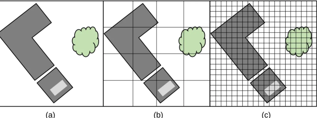
The spatial resolution or ground sampling distance is the size of the earth surface covered by one image pixel. For latest sensor systems like IKONOS, QuickBird, GeoEye-1, WorldView-2, or WorldView-3 it can reach up to a few meters or sub meter resolution (Momeni et al., 2016: 2). An object of interest can only be identified in the image domain, if the ground sampling distance is smaller or roughly equals its size (Blaschke, 2010: 3f). Generally, a scene is referred to be under-sampled when objects of interest are much smaller than the ground sampling distance, and over-sampled when the object of interest is much greater than the ground sampling distance (Fig. 1) (Momeni et al., 2016: 2f). In Very-High-Resolution (VHR) data, objects are most commonly over-sampled. This avoids mixed pixels and makes identification of objects at finer spatial scales possible. It therefore bares potential to produce more accurate classification maps and creates the possibility to investigate on smaller objects of interest. However, new challenges arise, as the highly detailed representation of objects increases intraclass- and reduces interclass heterogeneity (Alpin and Smith, 2011: 870; Momeni et al., 2016: 2f). Typical urban examples are ventilation or air-conditioning systems on rooftops. As they cover several pixels showing spectral profiles that differ from the rest of roof areas, they introduce intraclass variance in a potential roof class. In addition, spectral resolution of VHR sensors is rather limited. Thematic classes thus tend to show similar spectral

2 profiles if they are of similar materials, e. g. road asphalt and some rooftop materials (Hamedianfat and Shafri, 2015: 3381).

Both these challenges are addressed by the Object-Based Image Analysis (OBIA) approach (Blaschke, 2010: 3ff; Stumpf and Kerle, 2011: 2565; Blaschke et al., 2014: 81ff). By replacing the pixels as element to be classified by pixel groups – so called image-objects – intraclass

heterogeneity can be reduced (Alpin and Smith, 2011: 870; Momeni et al. 2016: 3). Additionally, indicators such as texture, shape, size, pattern and association derived for each image-object can supplement spectral information and increase interclass differences (Hamedianfat and Shafri 2015: 3381). Besides the shift to image-objects, non-parametric classifiers such as Support Vector Machines (SVM) increasingly substitute the statistical parametric methods like the Maximum Likelihood classifier (Melgani and Bruzzone, 2002, 2004; Foody and Mathur, 2004; Mountrakis et al., 2011: 249ff; Camps-Valls and Bruzzone, 2005, 2009; Salcedo-Sanz et al., 2014). Methods like SVM do not imply statistical assumptions on the data and therefore perform better on rather noisy data of complex environments (Momeni et al., 2016: 3).

Despite these proceeding concepts, still the quality of classification appears often strongly connected to user interaction (Lu and Weng, 2007: 825). This is especially true for supervised classification, where labeled samples need to be provided for learning a classification model (Fernandez et al., 2014: 4690). The labeled samples, referred to as ground truth data, are often sparse and can be costly as they might need to be generated through manual photointerpretation. Also, they can be limited by external sources, for instance availability of in-situ data (Dópido et al., 2013: 4032; Izquierdo-Verdiguier et al., 2013: 981). When working on complex and heterogeneous areas, gathering sufficient ground truth data can therefore become difficult (Lu and Weng, 2007: 825). This problem is confronted by several strategies.

Blaschke, 2010

Fig. 1: Relationship of ground sampling distance with object of interest. (a) Objects of interest appear under sampled. (b) Ground sampling distance corresponds roughly the size of the object of interest. (c) Objects of interest appear over sampled. Adapted from Blaschke (2010: 3).

3 The semi-supervised classification exploits unlabeled data (Dópido et al., 2013; Li and Zhou, 2015; Lu et al. 2016) while active- and relearning produce intermediate classification results which are reused for enhancement of the thematic map accuracies (Tuia et al., 2009b, 2011; Geiss and Taubenböck, 2015). They improve the performance in numerus settings but can potentially lead to a decrease in performance for other cases (Li and Zhou, 2015: 175). In the field of pattern recognition DeCoste and Schölkopf (2002) introduce so-called invariant SVM to confront related problems in the context of handwritten digit identification. Classification outcome is improved by including artificial samples into model training, which carry variations of characteristics not present in ground truth data but expected to occur in the data to classify. Izquierdo-Verdiguier et al. (2013) successfully transferred this approach to remote sensing using patch-based classification. However, determination of the variances appears challenging and time consuming. Yet, they are substantial to the approach as basis for encoding additional information, adapted to each class- and scene-specific task (Izquierdo-Verdiguier et al., 2013: 982).

Against this background, this thesis introduces a classification strategy to confront presented challenges linked to classification of VHR images and limited ground truth data. It aims on providing assistance where large ground truth data sets are not available or limited through barriers like time or cost effort of in-situ surveys. The approach combines OBIA and invariant SVMs and benefits from characteristic improvements each method implies. Therefore, section 2 introduces OBIA and its principle components, while section 3 presents the theoretical background and application of SVMs in general but also for invariant SVMs specifically. Section 4 gives a detailed explanation of the proposed approach and its functionality which is tested on a set of experiments presented in section 5. The results are summarized in section 6 and potential findings discussed in section 7. This thesis closes with final conclusions and an outlook for further investigation.

4

2 OBJECT-BASED IMAGE ANALYSIS

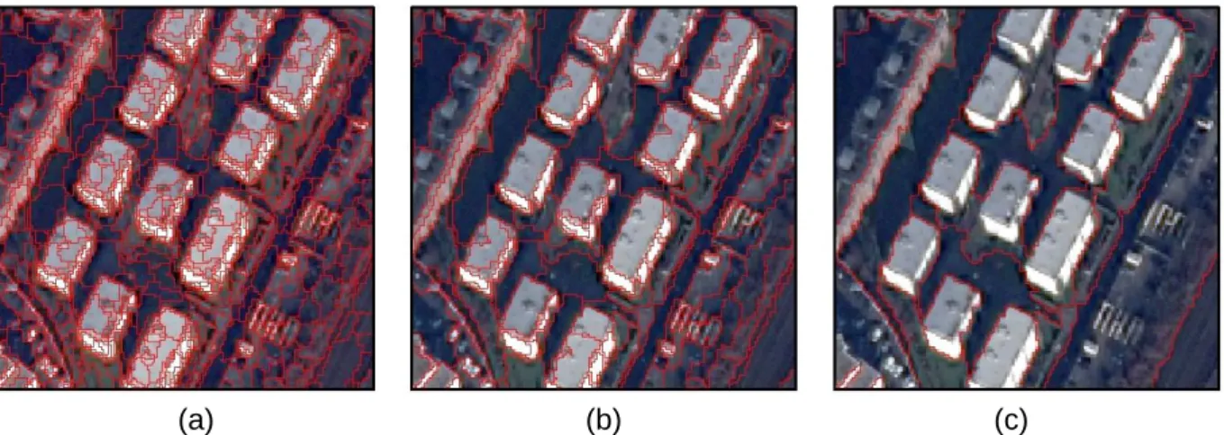
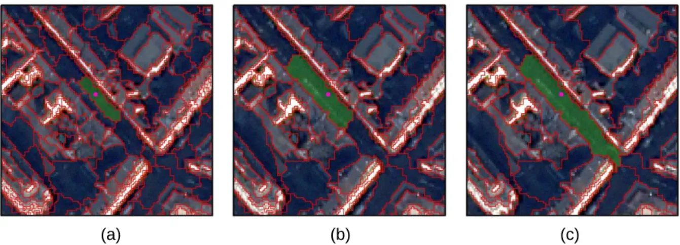
The OBIA approach, inspired by the human perception and interpretation of images, is founded on the assumption that an image is composed by interrelated objects of different size and shape (Bruzzone and Carlin, 2006: 2588; Lang, 2008: 6). The idea is to model such image-objects within the image domain to represent objects of interest with high accuracy. Subsequently a classifier labels the whole image-object instead of a single pixel. This bears the advantage that in the classification process spectral information can be supported by the mentioned object indicators describing the texture, shape or size of the image-objects. As this enhances the distinguishability of different land cover classes, better classification results can be achieved. Notably the nature of objects of interest can differ greatly, depending on the aim of the application and scene under investigation. Classification tasks might focus on single building types (Momeni et al., 2016) or tree species (Bunting and Lucas, 2006) while others aim on classifying urban agglomerations (Jacquin et al., 2008) or forest areas (Dorren et al., 2003). Castilla and Hay (2008) define the basic units of OBIA. The ‘image-object’ is considered as “a discrete region of a digital image that is internally coherent and different from its surroundings” (Castilla and Hay, 2008: 94). However, they extend this definition regarding semantic meaning. Seeing the image-object in relationship to the object of interest, there are generally three cases considered: First, oversegmentation, where the object of interest is represented by more than one image segment (Fig. 2a). Second, the ideal case, where the object of interest appears well modelled by the image segment (Fig. 2b) and third, undersegmentation,where more than one object of interest is represented by only one image segment (Fig. 2c) (Liu and Xia, 2010: 187f). For an oversegmented object of interest potentially characteristic information might remain unexploited, however produced information is valid and is likely to contribute to the enhancement of the classification result. This is not the case for undersegmentation. The image segment than carries information of two or more different objects of interest and hence two or more different information classes. If this segment is used

(a) (b) (c)

Fig. 2: Image segments in relation with objects of interest. (a) oversegmentation. (b) well modelled image segments. (3) undersegmentation. Own figure. Subset of Satellite Image: DigitalGlobe, (2014).

5 as entity to be classified and gets assigned to a land cover class, by default some part of the image-object gets misclassified and thereby corrupts the classification result (Liu and Xia, 2010). This consideration leads to the extension of the ‘image-object’ definition by the constraint that image-objects show barely oversegmentation and no undersegmentation regarding the objects of interest (Castilla and Hay, 2008: 96f).

The next two sections will focus on how those meaningful image-objects are generated through image segmentation and which characteristic indicators, so called features, can be derived from them to enhance distinguishability of different classes.

Image Segmentation

The image segmentation evolved to an essential part of OBIA as it generates the building blocks of the analysis – the image-objects (Blaschke, 2010: 3; Stumpf and Kerle, 2011: 2567). The purpose of segmentation algorithms is to partition the image into segments by merging neighboring homogenous pixels together and therefore making a differentiation between heterogeneous neighboring regions possible (Schiewe, 2002; Taubenböck et al., 2010: 121). In different segmentation strategies, homogeneity can be defined by different pixel or region properties, like spectral or spatial characteristics. For instance, pixels of water bodies typically show similar spectral properties, especially in the wavelength ranges of near-infrared. A segmentation procedure which gives the spectral characteristics on this band more weight concerning the homogeneity measure, will consequently perform well in modelling lakes or water-ways. In this sense, resulting segments are image regions created by one or several homogeneity criteria in one or several dimensions of feature space (Schiewe, 2002; Blaschke, 2010: 3). The outcome of the procedure must correspond to the stated requirements of image-objects as their information is subsequently used to enhance the image classification (Blaschke, 2010: 4). Segmentation algorithms used in remote sensing applications form four families: point-based, edge-based, region-based and combined approaches (Schiewe, 2002). For a more general overview of basic principles and application of the different methods Schiewe (2002) as well as Dey et al. (2010), among others, provide further readings.

This work makes use of a bottom-up region-merging segmentation algorithm, namely Multi-Resolution Image Segmentation (MRIS), which can be accounted to the region-based approaches (Benz et al., 2004). The algorithm has been applied successfully in numerous studies (Dey et al., 2010: 38). It allows the user to regulate the relative size of generated image segments through the definition of the maximal tolerated heterogeneity within the image segment by setting the so-called scale parameter. Additionally, by the parameters shape and compactness, it is defined to which extend spectral or spatial attributes influence the partition (Fig. 3) (Benz et al., 2004: 246f).

6 The algorithm starts at the pixel level, considering each pixel as a separate image segment. A pairwise clustering process then merges the two segments that produce the minimum global growth of heterogeneity. Step by step this merging process generates larger segments until the smallest growth of heterogeneity surpasses the user defined scale parameter. A formal definition of the procedure is provided by Benz et al. (2004) and Bruzzone and Carlin (2006). Merging of image segments follows the bottom-up approach, where segments and their borders are never created entirely new but only formed by the union of two already existing segments. This proceeding makes it possible to create not only one segmentation map, but to define a set of scale parameters and create a set of unambiguous hierarchically related segmentation maps for the same image. They satisfy the constraint

⋃ 𝑂𝑖𝑠 = 𝑂𝑗𝑠+1 𝑂𝑖𝑠⊆𝑂𝑗𝑠+1

(1)

where at the segmentation level 𝑠 the image is subdivided in 𝑁𝑠_{objects 𝑂}

𝑖𝑠 (𝑖 = 1, 2, … , 𝑁𝑠) (Bruzzone and Carlin, 2006: 2590; Geiss and Taubenböck, 2015: 2337). In other words, the constraint guarantees that any object at level 𝑠 − 1 cannot be part of more than one object in level 𝑠. This modelling of hierarchical relation between objects of different segmentation levels makes it possible to not only substitute the pixel as image analysis element with the object, but to add object information from different levels to hierarchically related analysis elements. The feature vector of the image-object in the lowest level gets extended by feature vectors of the objects enclosing it at higher levels. Additionally, further object indicators concerning pattern Fig. 3: Concept of Multiresolution Image Segmentation. Composition of object homogeneity and influence of the scale parameter. Adopted from eCognition (2016: 71).

Composition of homogeneity Homogeneity criteria derived for each image-object and potential unions of image-objects.

Colour

Defines homogeneity of spectral properties. Composed by band values. Weight: 1 – shape

Shape

Defines the weight of object shape in the homogeneity criteria. Composed by compactness and smoothness.

User defined weight: [0 - 0.9] Scale

Defines the maximum heterogeneity in image-objects in reference to the homogeneity criteria.

Object sizes increase with higher scale value. User defined: [0 -∞]

Smoothness

Criteria of smoothness from the border outline of image-objects. Weight: 1 – compactness

Compactness Criteria of the overall

compactness of image-objects. User defined weight: [0 - 1]

7 and association become available. Bruzzone and Carlin (2006: 2588) state that by considering such hierarchical sets of segmentation maps in the classification system, it is possible to analyze each real-world object at its optimal representation level. Also, it takes into account that objects are logically interrelated within the same level and hierarchically related to those in higher or lower levels. This concept is referred to as multilevel object-based classification.

Image-Object Features

Object features, also referred to as object metrics, carry the information that describes each object and builds the foundation to determine the classification rules. They construct the so-called feature space. The term refers to a space, where each feature measure is considered a dimension. If objects are, for example, characterized by only three features, the pixel values blue, green and red, the feature space is 3-dimentional and each object has its definite position within it – specified by the coordinates blue, green and red. Therefore, the number of considered features defines the dimensions of feature space.

Combining aspects like shape, size, pattern, tone, texture, shadow and association makes object identification by human vision possible (Olson, 1960; Blaschke et al., 2014: 182). In this sense, a diverse pool of object features arose concerning spectral and geometry-related properties, including texture, but also encoding topological information like neighborhood and hierarchical relation (Bruzzone and Carlin, 2006: 2591; Blaschke, 2010:10; Geiss et al., 2016b: 5952). In the following, the focus is on different feature types that encode spectral, textural and spatial characteristics. After a brief introduction for each group, the measures selected for this study are discussed in more detail.

2.2.1 Spectral

Spectral information refers to the reflection behavior of different real-world objects. Therefore, spectral information can be exploited by analyzing directly the numerical values of each available spectral band (Bruzzone and Carlin, 2006: 2591) and additionally calculated band ratios like the Normalized Differenced Vegetation Index (NDVI, (𝑛𝑒𝑎𝑟 𝑖𝑛𝑓𝑟𝑎𝑟𝑒𝑑−𝑟𝑒𝑑)

(𝑛𝑒𝑎𝑟 𝑖𝑛𝑓𝑟𝑎𝑟𝑒𝑑+𝑟𝑒𝑑)) (Rouse et al., 1973). For this study, the statistical measures of central tendency and spread, mean and

standard deviation, of pixels included in an image-object are calculated for each spectral band and the stacked NDVI correspondingly and used for spectral characterization of the image-object.

8

2.2.2 Texture

Texture refers to the frequency of tone variance, i.e. spectral band values and the spatial arrangements of those variances (Hay and Niemann, 1994; Pacifici et al., 2009: 1277; Blaschke et al., 2014: 183). Especially in scenarios with limited spectral resolution, as it is the case for VHR or panchromatic imagery, it has been demonstrated that the use of textural features has great potential for the improvement in classification accuracies (Zhang et al., 2003; Carleer and Wolff, 2006; Laliberte and Rango, 2009; Pacifici et al., 2009).

The Grey-Level Co-occurrence Matrix (GLCM) method (Haralick et al., 1973; Haralick, 1979) is well established for texture characterization in remote sensing and successfully used in many studies (Zhang et al., 2003; Pacifici et al., 2009; Stumpf and Kerle, 2011). All GLCM measures are based on a symmetric matrix, which counts grey-level co-occurrences of directly neighboring pixels for all pixels within the image-object. This approach makes it possible to recognize specific patterns or arrangements of reflectance intensity. By summarizing those matrices using different functions, a variety of texture measures for the image-object can be created. In order to keep the feature set compact, but also in consideration of the high computational burden and strong correlations between many GLCM measures (Cossu, 1988; Laliberte and Rango, 2009), the set of GLCM textural features for this study is limited to

homogeneity, dissimilarity and mean. Homogeneity returns high values whenever an object shows low variance in its pixel grey-levels, hence is high for homogeneous objects (Pacifici et al., 2009: 1281). Dissimilarity is a measure of contrast within the image-object, while mean is the mean of the co-occurrence matrix and thus the mean co-occurrence of all present grey-levels. Their formal definitions are provided in the following according to the implementation in the used software eCognition (eCognition, 2016: 412ff):

ℎ𝑜𝑚𝑜𝑔𝑒𝑛𝑒𝑖𝑡𝑦 = ∑ 𝑃𝑖,𝑗 1 + (𝑖 − 𝑗)2 𝐺−1 𝑖,𝑗=0 , (2) dissimilarity = ∑ 𝑃𝑖,𝑗|𝑖 − 𝑗| 𝐺−1 𝑖,𝑗=0 , (3) 𝑚𝑒𝑎𝑛 =∑ 𝑃𝑖,𝑗 𝐺−1 𝑖,𝑗=0 𝐺² . (4)

𝐺 is the number of grey-level values present in the image-object and therefore the amount of rows or columns in the corresponding co-occurrence matrix. 𝑖 and 𝑗 are the coordinates in the matrix and 𝑃𝑖,𝑗 is the normalizes value at the position 𝑖, 𝑗 within the matrix, hence the normalized frequency of the co-occurrence of grey-level pair 𝑖, 𝑗 within the image-object.

9

2.2.3 Shape

Shape features are measures that describe the outline or general form of the individual image-object (Blaschke et al., 2014: 182). Especially in applications aiming to detect man-made objects, like the classification of urban environments, this group has great potential to improve classification results (Sun et al., 2015: 3737). This is due to the fact that man-made objects often show regular boundaries, which are rarely found with natural objects. For this study, shape related properties are therefore considered by the indices rectangular fit, elliptic fit, roundness, shape index and compactness. The rectangular fit and elliptic fit are based on the same principle:

𝑟𝑒𝑐𝑡𝑎𝑛𝑔𝑢𝑙𝑎𝑟 𝑓𝑖𝑡 = 𝐴𝑅 𝐴𝑂 , (5) 𝑒𝑙𝑙𝑖𝑝𝑡𝑖𝑐 𝑓𝑖𝑡 = 𝐴𝐸 𝐴𝑂 , (6)

with 𝐴𝑂 being the area of the image-object and 𝐴𝑅 its intersection with a rectangle having identical area and its proportion rotated to the original objects shape moments. 𝐴𝐸 is the intersection with an ellipse having similar properties respectively (Sun et al., 2015: 3738ff).

Roundness is calculated by

𝑟𝑜𝑢𝑛𝑑𝑛𝑒𝑠𝑠 = 𝜀𝑚𝑎𝑥− 𝜀𝑚𝑖𝑛 (7)

where 𝜀𝑚𝑎𝑥 _{is the radius of the smallest, the image-object enclosing ellipse and 𝜀}𝑚𝑖𝑛_{the radius} of the largest, by the image-object enclosed ellipse. Shape index describes the smoothness of the image-objects borders and is mathematically expressed as

𝑠ℎ𝑎𝑝𝑒 𝑖𝑛𝑑𝑒𝑥 = 𝐿𝑂 √𝐴𝑂

4 (8)

where 𝐿𝑂 is the border length of the image-object. Compactness is defined by

𝑐𝑜𝑚𝑝𝑎𝑐𝑡𝑛𝑒𝑠𝑠 = 4 ∗ 𝜋 ∗ 𝐴𝑂 𝐿𝑂2

(9)

with 𝐿𝑂 being the perimeter of the image-object. Therefore, for the most compact shape – the circle – returns the highest value: one.

Sun et al. (2015) point out that the extraction of shape information from image-objects can be improved in reference to these traditional shape features. Blaschke et al. (2014: 182) however argue that shape features may often not be inherently distinctive, but can appear as important factor in diverse composed feature sets.

10

3 SUPPORT VECTOR MACHINE CLASSIFICATION

In this section, the SVM algorithm is briefly reviewed and its principal functionality is discussed as the method proposed in chapter 4 builds on some SVM specific properties. However, for a more extensive, general introduction it is referred to Cortes and Vapnik (1995), Burges (1998), Vapnik (1998), Schölkopf and Smola (2002) and Foody and Mathur (2004), while remote sensing specific literature is provided by Melgani and Bruzzone (2004), Camps-Valls and Bruzzone (2005, 2009), Mountrakis et al. (2011) and Salcedo-Sanz et al. (2014).

Theoretical Background

The Support Vector Machine, first introduced by Cortes and Vapnik (1995) in the field of machine learning, constitutes a group of non-parametric supervised classification and regression approaches.

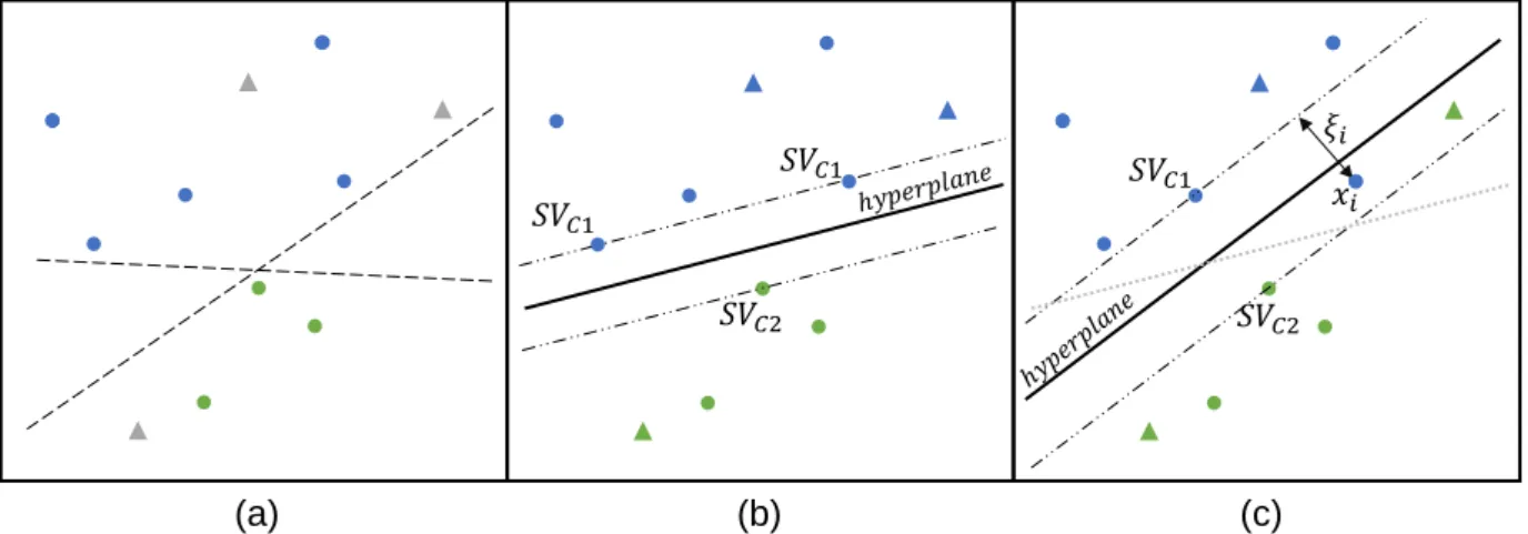
For a binary supervised classification problem, the SVM seeks to find the optimal decision surface, also called optimal separating hyperplane, which separates the instances of the two classes in feature space (Burges, 1998). As input, labeled samples for each class need to be provided. On the basis of this set of labeled samples, the SVM is learned. A great number of hyperplanes might be able to separate the samples of the two classes (Fig. 4a). However, by choosing the one that lies in the center of the widest sample free corridor, it is assumed that the separation is more likely to be valid for unseen data points. In this sense the optimal decision surface is the one that maximizes a margin formed by two additional surfaces lying parallel to the decision surface and intersecting the samples closest to it (Fig.4b). These samples lying on the margin border are called Support Vectors (SV) (Burges, 1998; Leinenkugel et al., 2011; Geiss et al., 2016a: 1922f). Unlabeled samples are located at either side of the optimal separating hyperplane and can thereby be labeled correspondingly

(a) (b) (c)

Fig. 4: Idealized process of locating the optimal separating hyperplane. Dots represent labelled training data of two classes (blue and green). Triangles represent new unseen instances (grey: unclassified, blue/green: classified correspondingly). (a) Available labelled instances for training. (b) Separation of instances by the hyperplane of the SVM. (c) Adaption to soft margin SVM, e.g. C-SVM. Adapted from Melgani and Bruzzone (2004: 1781); Izquierdo-Verdiguier et al. (2013: 982).

Melgani and Bruzzone 2004

11 (Fig. 4b). It is important to stress that the SVs do carry all the information needed to define the optimal hyperplane and hence to build the decision function. Robust models which generalize well can therefore already be derived from relatively small training set sizes (Geiss et al., 2016a: 1922f).

Considering a set of labeled training samples 𝑆 = {𝑋, 𝑌}, where 𝑋 = {𝑥𝑙}𝑙=1𝑛 ∈ ℝ𝑑 are 𝑛

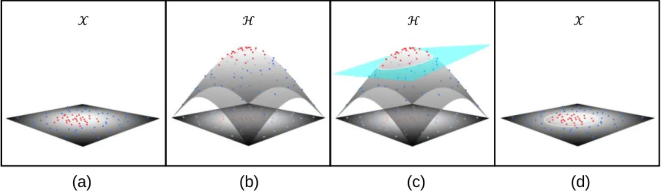
𝑑-dimensional feature vectors associated with the labels 𝑌 = {𝑦𝑙}𝑙=1𝑛 ∈ {−1, 1}, suitable parameters are found to define the optimal separating hyperplane during training of the SVM (Camps-Valls and Bruzzone, 2005: 1353; Geiss et al., 2016a: 1930ff). As data is rarely linear separable, meaning an accurate linear separation by a hyperplane of information classes is not possible, a nonlinear transformation 𝜙(⋅) maps the labeled samples from the original feature space 𝒳 into a space of higher dimensionality ℋ. This is helpful as linear separation in ℋ can be easier to achieve and matches a potentially high complex nonlinear separation in

𝒳 (Fig. 5). In this sense, mapping by an appropriate 𝜙(⋅) makes instances of the two classes more likely to appear separable. Yet, if the data to classify is very noisy or classes appear to have great overlap in feature space, it can be convenient to allow misclassification of some samples with the aim of widening the margin and the generalization capacity. This is implemented by a so-called slack variable and a penalty factor 𝐶 (Fig.4c) (Cortes and Vapnik, 1995: 280ff; Geiss et al., 2016a: 1931f). In these cases, literature speaks of soft margin classifiers implemented as C-SVM because the margin is “softened” as it allows samples to appear on the wrong side of the hyperplane, but each misclassification gets penalized by a defined factor 𝐶. In other words: if factor 𝐶 is chosen very large the model tempts to overfit on training data, because misclassification is highly penalized and therefore rare. While in the contrary case, the model may allow too many misclassified samples which cause underfitting (Ben-Hur and Weston, 2010: 7ff). As both cases produce poor results on unseen data, the

Blaschke, 2010

ℋ ℋ 𝒳

𝒳

Fig. 5: Idealized process of defining a nonlinear decision function by SVMs. (a) Samples of two classes, red and blue dots, that are not linear separable in 𝒳. (b) Samples are mapped by the nonlinear transformation 𝜙(⋅) to the higher dimensional space ℋ. This makes linear separation by a hyperplane (cyan) possible, which is fitted by maximising the margin (c). In input space 𝒳 this separation corresponds a nonlinear decision function (d). From Geiss et al. (2016a: 1931).

12 penalty factor 𝐶 must be determined carefully. On this foundation, the method delivers a decision function optimized on the training data in the form of:

𝑓(𝑥∗) = 𝑠𝑔𝑛 (∑ 𝑦𝑖 𝑛

𝑖=1

𝛼𝑖𝐾(𝑥𝑖, 𝑥∗) + 𝑏) (10)

with 𝑥∗ being an instance of unidentified class membership, 𝑥𝑖 being the 𝑖th of 𝑛 support vectors with corresponding label 𝑦𝑖 and support vector coefficient 𝛼𝑖. Those coefficients and the bias of the hyperplane 𝑏 are defined during the optimization process, hence the training of the classifier on the labeled samples, and encode also the influence of 𝐶 on the decision function (Cortes and Vapnik, 1995; Camps-Valls and Bruzzone, 2005; Gehler and Schölkopf, 2009). The decision function 𝑓(𝑥∗) depends on the underlying data through the dot product of the mapped instances. The dot product can be replaced by a kernel function 𝐾(𝑥𝑖, 𝑥𝑗) =

𝜙(𝑥𝑖), 𝜙(𝑥𝑗) that returns the similar result and thereby the explicit calculation of any mapping

𝜙(⋅) can be avoided. This is known as the kernel trick (Gehler and Schölkopf, 2009: 27). This property allows the SVM algorithm to efficiently compute the decision function also for high dimensional data, as costly mapping by 𝜙(⋅) can be spared. While there are several different kernels with a variety of characteristics, the one commonly used for environmental applications is the Gaussian Radial Basis Function (RBF) kernel which takes the form of

𝐾(𝑥𝑖, 𝑥𝑗) = exp (−𝛾 ||𝑥𝑖− 𝑥𝑗|| 2

) (11)

(Bruzzone and Carlin, 2006: 2592; Volpi et al, 2013: 80). 𝛾 > 0 thereby controls the width of the Gaussian. In this sense, 𝛾 determines the flexibility of the SVM in fitting on the training data. A high 𝛾 value can be seen as great flexibility and therefore ‘tight’ fitting on labeled samples, which in consequence can lead to overfitting. But for a too low 𝛾 value the SVM might not be flexible enough to model a complex classification setting (Ben-Hur and Weston, 2010: 7ff). Again, the parameter needs to be set according to the classification problem. Consequently, regarding the application of the C-SVM in combination with the RBF kernel, it is essential for good performance – meaning good generalization on unseen data – that the two hyperparameters 𝐶 and 𝛾 are carefully chosen.

In remote sensing, classification tasks often consider a variety of land cover classes. The SVM, originally designed to solve binary classification, therefore needs to be effectively extended to multiclass problems. The one-against-one approach is a suitable strategy to solve this problem (Hsu and Lin, 2002: 425). For 𝑘 information classes a total number of 𝑘(𝑘 − 1)/2 binary classifiers are trained, representing each possible binary class combination. A label of an unclassified sample is then predicted by each classifier and subsequently keeps the label with the highest count of assignments (Hsu and Lin, 2002; Foody and Mathur, 2004: 1337).

13

SVMs in Remote Sensing

Mountrakis et al. (2011) point out benefits and challenges of SVMs in remote sensing: A key characteristic is the relatively high classification accuracy on small training data sets, compared two traditional methods (Mantero et al., 2005; Mountrakis et al., 2011: 248). In various settings, the limited number of training instances is combined with a very high dimensionality of the same. This is especially true for hyperspectral datasets (Melgani and Bruzzone, 2004; Camps-Valls and Bruzzone, 2005), but also applies for OBIA (Bruzzone and Carlin, 2006; Tuia et al., 2009a; Cánovas-García and Alonso-Sarría, 2015). In these settings, classification results are prone to suffer the so-called Hughes phenomena (Hughes, 1968). It describes the problem of training sets in which the feature dimensionality is much greater than the number of samples. This typically leads to a decrease in accuracy with increasing feature dimensionality. However, the SVM classifier has shown relatively high robustness to the Hughes phenomena and hence, feature reduction analyses which is needed in other approaches, can be spared (Melgani and Bruzzone, 2004: 1779; Gualtieri, 2009). SVMs are non-parametric classifiers, meaning there is no assumption made on the statistical distribution of the underlying data and all function parameters are derived in connection with provided training data. Burges (1998) demonstrated that, since the distribution of the remote sensing data is usually unknown (Mountrakis et al., 2011: 248), this can be an advantage over parametric classifiers, like the Maximum Likelihood Estimation. Another advantage quoted by Mountrakis et al. (2011) concerns the problem of overfitting on the training data. The method has shown good balancing of accuracy achieved on the training patterns and the capacity to generalize well on unseen instances. Opposed to these advantages, there are several barriers that hinder the application of SVMs. The greatest involve the choice of the used kernel as well as a deeper understanding of many model variants and adaptations for more specific tasks (Mountrakis et al., 2011: 248). To tackle such difficulties a wide range of SVM tutorials is provided in literature (Cortes and Vapnik, 1995; Burges, 1998; Ben-Hur and Weston, 2010). Nevertheless, SVM has become a standard tool in processing and classification of remote sensing data (Izquierdo-Verdiguier et al., 2013: 981). Relevant to this thesis, is the effectiveness of the method in combination with on one side OBIA, on the other semi-supervised approaches that deal with artificial samples to overcome restrictions of sparse ground truth data on VHR imagery.

Concerning the first, Momeni et al. (2016) performed an extensive experiment comparing different spatial resolutions, classifiers and feature sets for a complex land cover classification task. They recommend a combination of OBIA with SVMs for spatially high resolution settings. Geiss et al. (2016a) report good results by combining OBIA with SVM for a multisource approach based on multispectral, elevation, spatial-temporal and in-situ data for seismic

14 vulnerability assessment. Fernandez et al. (2014) found that the SVM and Nearest Neighbor method produce the most accurate and robust classification of impervious surface areas by means of OBIA. Yet, it is stated that distribution and size of the training data sets still play a key role in classification results (Foody and Mathur, 2004: 1340; Fernandez et al., 2014: 4690). In the field of semi-supervised classification Bruzzone et al. (2006), Gómez-Chova et al. (2011) and Li and Zhou (2015) modify the basic SVM formulation to deal with unlabeled data, while Dópido et al. (2013) and Lu et al. (2016) include the principal of self-learning in their approaches, where the most informative unlabeled samples are selected by the machine learning algorithm itself. Li and Zhou (2015) also point out that in some cases semi-supervised learning methods appear to show worse performances as supervised classification. Their work focuses on this issue and proposes SVM variants of higher reliability while handling unlabeled data. An alternative approach to sparse training data is to incorporate prior knowledge of the data representation into the classification model, namely in form of invariant SVM.

Invariances in SVMs

The term ‘invariance’ refers to a specific property of a mathematical function. An algorithm implementing such a function is called ‘invariant’. It means that the algorithm, let it be a classifier, is robust to changes in the data representation (Izquierdo-Verdiguier et al., 2013: 981). To give a simple example, a classifier with the task to detect buildings is considered. Let the training data only include instances of buildings with quadratic shape. However, it is desirable that also buildings with a rectangular shape are recognized, as this might occur in the data to classify. If this prior knowledge about changes within the data representation, is incorporated in the classifier and enables it to manage the classification task, the classifier could be considered invariant to the shape of the buildings. Originally, encoding invariance in SVM classifiers was presented by Schölkopf et al. (1996), DeCoste and Schölkopf (2002) and Chapelle and Schölkopf (2002). DeCoste and Schölkopf (2002) show the effectiveness of two main approaches on handwritten digit recognition, but also by the identification of volcanos in preselected satellite image patches. While one exploits engineering of kernel functions that results in invariant SVMs, the second focuses on the training data. Due to its effectiveness and simplicity, this work concentrates on the latter approach. DeCoste and Schölkopf (2002) state that it is essential to have access to prior knowledge about desired invariances or in other words, the variance that might occur in data. On the basis of this knowledge, instances from the training set can be transformed to encode desired characteristics and reincluded in model training. Such a model trained on transformed and original samples should appear invariant to the included characteristics. For the given example, instances that represent quadratic houses are modified to rectangular shape and reincluded in the model. The resulting classifier, trained on original quadratic and artificial rectangular houses, will then recognize both shapes during classification and therefore improve the quality of classification. As the calculated decision

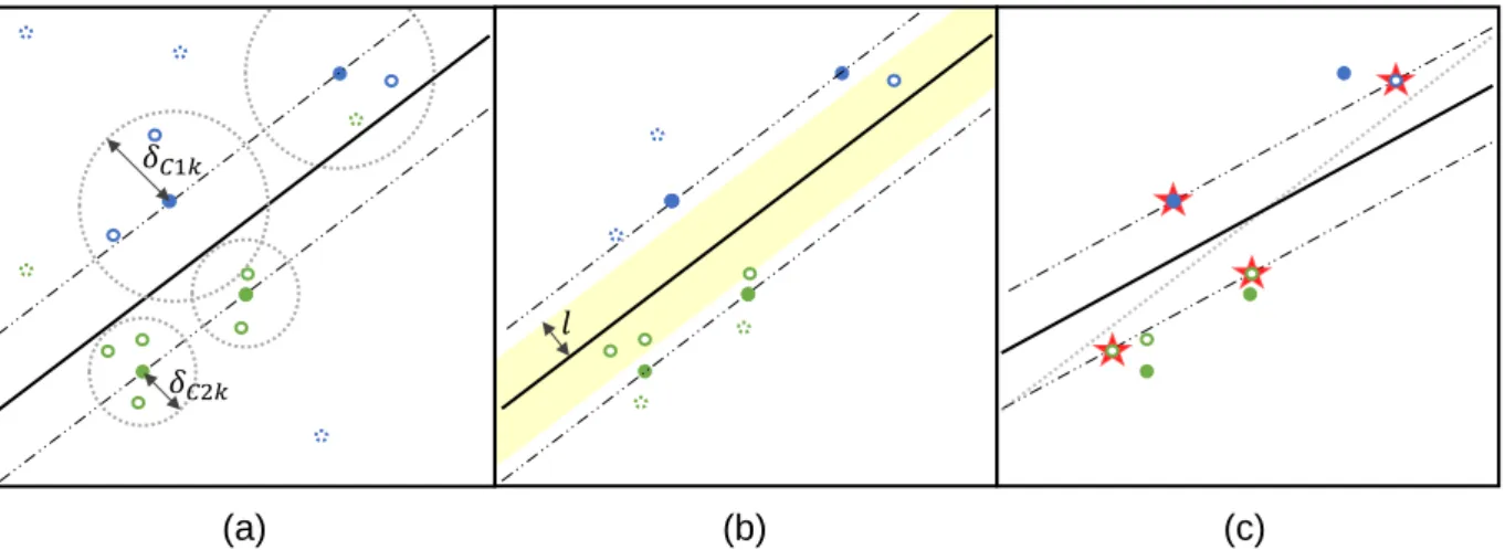
15 function of a SVM only relies on the SVs, it is sufficient to exclusively apply the transformation of instances to the model SVs. Artificial samples, resulting out of the transformation process, are called Virtual SVs (VSVs). The invariant SVM, trained on SVs of the initial model and generated VSVs, is referred to as Virtual SVM (VSVM). In summary, this leads to the following general process (DeCoste and Schölkopf, 2002:165):

1. train an initial SVM on some training set and extract its SVs (Fig. 6a, b)

2. transform SVs to VSVs so that they carry the information to which the model shall be invariant

3. train a second VSVM on the set of SVs and VSVs (Fig. 6c)

VSVs should appear close to the separating hyperplane as they derive from samples lying on the margin borders. Therefore, they are likely to become SVs during the second training and shift the hyperplane to be robust to the encoded change in data representation (Fig. 6c) (DeCoste and Schölkopf, 2002).

Izquierdo-Verdiguier et al. (2013) transfer this approach to patch-based classification for VHR remote sensing data. They encode invariance to rotation and scale of real-world objects as well as to appearance of shadow in the image. VSVs are generated by rotating or up- and downscaling the image patches and by remodeling reflectance values for samples of the shadow class. All three experiments showed the effectiveness of the method with an improvement of 5-7% in 𝜅 accuracy. However, the authors note that prior knowledge of variances that may appear in unseen data and the appropriate encoding of this knowledge into VSVs is of paramount importance.

Fig. 6: Simplified functionality of VSVMs. Dots represent labelled training data of two classes (blue /green). Triangles represent new unseen instances (grey: unclassified, blue/green: classified). Circles represent VSVs of each class (blue/green). (a) Available labelled instances for training. (b) Initial trained SVM model. (c) VSVM model with VSV and shifted optimal separating hyperplane. Adapted from Izquierdo-Verdiguier et al. (2013: 982).

(a) (b) (c)

DeCoste and Schölkopf 2002

𝑆𝑉 1

𝑆𝑉 ₂ 𝑉𝑆𝑉𝑠 2

16

4 INVARIANCES IN SUPERVISED OBJECT BASED CLASSIFICATION

In aforementioned approaches for VSVMs, the encoding of prior knowledge is realized by strong interaction with the expert user. Next to the identification of the desired invariance, the degree of its manifestation needs to be set. Izquierdo-Verdiguier et al. (2013) defines a realistic scale variance of tree sizes from 50-120% of the labeled samples and encodes those values in the up- and downscaling of the image-patches. It means that prior knowledge needs to be existent or generated by the expert user and implemented according to each setting.

On this basis, in this section the principal structure is introduced that combines OBIA with VSVM classification. It is proposed in a way that is generally applicable to different classification tasks and data sources, if feature sets and information classes are adapted. Redetermination and reimplementation of possible invariance characteristics for each classification task are not necessary. While the invariance type is pre-set to scale and geometry, definition and encoding of the actual range of variance in data is replaced by the use of image segmentation. While section 4.1 specifies understanding of scale and geometry invariance in this work, section 4.2 presents the actual implementation.

Invariance in Scale and Geometry

Considering OBIA in complex, heterogeneous scenes, and for the case of sparse ground truth data, it is probable that some classes are only represented with a subset of its existing object sizes in the training set. Potential reasons include a limited number of labeled instances or over- and undersegmentation within the same segmentation map. Both conditions make optimal representation of all real-world objects impossible (Schiewe 2002: 3). Especially in an urban environment, where man-made objects can differ significantly in size – from a parking lot of a detached house to a city square (potential impervious surfaces land cover class) or from a single tree to a city park complex (potential vegetation land cover class) – scale invariance is expected to improve classification results. It means that these different scale variation of real-world objects are recognized by the classifier even if they are not present in available ground truth data. The same accounts for the geometry of objects. Houses can build stretched forms if they are built in closed rows or compact forms for single housing. Impervious surfaces are formed by stretched or compact shapes, from long and slim roadways to more compact polygons of open places. Also for scenes with unbalanced geometry characteristics – in which some classes show great geometric variety, while others are rather homogenous, geometry invariance implemented for each class accordingly is expected to enhance results. In OBIA, segmentation determines the image-objects and therefore scale and geometry attributes. A logical consequence is to approach variations of scale and geometry by using a segmentation procedure. Through a variety of parameter settings for the segmentation

17 algorithm, a collection of scale and geometry representations of different objects can be achieved and used to encode invariance.

Proposed Methodology

The procedure follows the principal steps of VSVMs introduced in section 3.3. Those are transferred to the remote sensing context as follows (Fig. 7): A typical OBIA segmentation procedure (MRIS) partitions the image domain in well modelled image-objects (section 4.2.2) for the training of an initial SVM (section 4.2.3). On the base of its SVs and by the use of segmentation maps created additionally by modifying the parameter of the MRIS used before, VSVs are created (section 4.2.4). The VSVs are evaluated by their quality of information to select only representative and non-redundant VSVs for the VSVM (section 4.2.5). Finally, the VSVM is trained and used for the classification of unseen data (section 4.2.6). For a good classification result of the SVMs, a strict separation of the labeled samples in training and testing data is necessary, which is explained and presented in section 4.2.1.

4.2.1 Ground Truth Data Sets

To learn the most accurate C-SVM with a RBF kernel the cost-parameter 𝐶 as well as the kernel-width parameter 𝛾 need to be defined. Generally, the optimization of this parameter combination can be solved by a grid-search strategy (Foody, 2009: 90). This means that for 𝐶

and for 𝛾 sequences of potential parameter values are defined. From these sequences, all parameter combinations are used to train a classifier on a subset of available labeled samples, while the remaining samples simulate unseen data to be classified and to evaluate Fig. 7: Block scheme of the proposed method. Own figure.

Segmentation Optimal Parameter Set Relearn Invariant VSVM Segmentation Modified Parameter Sets Learn Initial SVM Extract SVs Classification Map Compute Object Features Identify Potential VSVs Compute Object Features Che c k of Red u n d a n c e Che c k o f Rep re s e n ta ti v ity Image Ground Truth Data

18 performance of parameter combination. The best performing parameter combination qualifies for the classification task and is used to train the final SVM. As it is desirable to use all the information carried by labeled samples, cross-validation is frequently and successfully applied in this step (Foody and Mathur, 2004; Tzotsos and Argialas, 2008; Foody, 2009; Gehler and Schölkopf, 2009: 38; Izquierdo-Verdiguier et al., 2013; Geiss et al., 2016a; Hsu et al., 2016). However, for this VSVM the number of VSVs can easily exceed the number of original samples by its multiple. This entails the danger of strong dominance of VSVs in the parameter setting process and therefore the risk of overfitting the model on the artificial samples, while the original SVs lose on influence. Additionally, VSVs are likely to show feature characteristics that resemble their original SV. Hence, a consistent separation and simulation of unseen data might be violated when using cross-validation on a sample set that contains SVs from the initial model and their VSV derivations. In other applications, similar problems are known as data leakage. As a result, the classifier produces high accuracies during the iterations of cross-validation, but performs poorly on unseen data.

This is avoided by using the hold-out method (Foody, 2009: 90) which implies splitting labeled samples into two spatially disjunct subsets. During grid-search procedure, the first subset is used for training and can be enriched by VSVs. The second subset consists of original samples and is used to estimate the accuracy measure for each parameter combination of 𝐶 and 𝛾. In the following, those distinct sets are referred to as 𝑡𝑟𝑎𝑖𝑛𝑆𝑒𝑡 and 𝑡𝑒𝑠𝑡𝑆𝑒𝑡.

4.2.2 Segmentation Procedure

The image segmentation used for the initial SVM requires a manual setting of parameters of the MRIS algorithm (scale, shape and compactness; Fig. 3). These are adjusted in reference to the criteria for image-objects presented in section 2 concerning over- and undersegmentation. Image-objects of this segmentation map will serve as the basis of the subsequent procedure. Therefore, the segmentation map will be referred to as 𝑠𝑒𝑔𝑏𝑎𝑠𝑒. For the purpose of introducing invariance, two additional sets of segmentation maps are derived from 𝑠𝑒𝑔𝑏𝑎𝑠𝑒. They are denoted by 𝑠𝑒𝑔𝑆𝑒𝑡𝑠𝑐𝑎𝑙𝑒 and 𝑠𝑒𝑔𝑆𝑒𝑡𝑔𝑒𝑜𝑚 for scale and geometry invariance respectively. Selected objects of those segmentation maps will serve as VSVs in the invariant model. 𝑠𝑒𝑔𝑆𝑒𝑡𝑠𝑐𝑎𝑙𝑒 is generated by keeping parameters of shape and compactness constant while altering the parameter of scale. It means that the weights for shape/color and compactness/smoothness, which define the composition of the heterogeneity in the image segments, are kept constant. Thereby their geometry is defined similar to the geometry of segments in 𝑠𝑒𝑔𝑏𝑎𝑠𝑒. However, the scale parameter defining the threshold for the composed maximum heterogeneity is altered, which influences the size of resulting segments. The sizes of image segments generated by different scale parameters may generally move between an upper and a lower bound. The latter fulfils good representation of the smallest and

19 most homogeneous real-world objects while accepting oversegmentation for others (typically small scale parameter). The upper bound is a good representation of the largest and very heterogeneous real-world objects while accepting undersegmentation for others (typically large scale parameter). 𝑠𝑒𝑔𝑆𝑒𝑡𝑔𝑒𝑜𝑚 is generated by modification of the shape and compactness parameter, while keeping the scale parameter of 𝑠𝑒𝑔𝑏𝑎𝑠𝑒 constant. This leads to segments of roughly the same size but different geometries compared to those of 𝑠𝑒𝑔𝑏𝑎𝑠𝑒. The variation of shape and compactness may be realized up to the point where generated segments lose the relation to outlines of real-world objects.

The aim of defining those bounds quite broad is to encode the entire spectrum of object-scale or object-geometry variety present in data for different land cover classes into image segments. As those image segments are used to make the classifier invariant, this appears crucial to the approach. The presence of over- and undersegmented objects is accepted, because the optimization procedure (introduced in section 4.2.5) chooses only valid instances from

𝑠𝑒𝑔𝑆𝑒𝑡𝑠𝑐𝑎𝑙𝑒 and 𝑠𝑒𝑔𝑆𝑒𝑡𝑔𝑒𝑜𝑚. The number and intervals of parameter variations can be regarded as a balance between computational burden and exploration of potential information. However, the usage of up to nine segmentation maps for 𝑠𝑒𝑔𝑆𝑒𝑡𝑠𝑐𝑎𝑙𝑒 and eight maps for 𝑠𝑒𝑔𝑆𝑒𝑡𝑔𝑒𝑜𝑚 proved to be appropriate in performed experiments.

Note that 𝑠𝑒𝑔𝑆𝑒𝑡𝑠𝑐𝑎𝑙𝑒 forms a typical multilevel representation of the image and meets equation (1), while 𝑠𝑒𝑔𝑆𝑒𝑡𝑔𝑒𝑜𝑚 violates equation (1) as it does not build a hierarchic structure. Image segments of one segmentation map cross borders of image segments of a second segmentation map as they do not differ greatly in size but in geometry. Consequences resulting out of this are discussed in section 7.

4.2.3 Basis SVM Classification

Although this work addresses invariance to scale and geometry, this section presents the method concerning scale invariance. Both procedures rely on the same principles and manner of implementation. Only the used set of segmentation maps, namely 𝑠𝑒𝑔𝑆𝑒𝑡𝑠𝑐𝑎𝑙𝑒 and

𝑠𝑒𝑔𝑆𝑒𝑡𝑔𝑒𝑜𝑚 distinguish the methods variation.

As the initial SVM on 𝑠𝑒𝑔𝑏𝑎𝑠𝑒 structures the foundation of the subsequent process, it will be referred to as 𝑆𝑉𝑀𝑏𝑎𝑠𝑒. 𝑆𝑉𝑀𝑏𝑎𝑠𝑒 is trained on given labeled image-objects of 𝑠𝑒𝑔𝑏𝑎𝑠𝑒 that are spitted in 𝑡𝑟𝑎𝑖𝑛𝑆𝑒𝑡 and 𝑡𝑒𝑠𝑡𝑆𝑒𝑡 for the hyperparameter optimization (𝐶, 𝛾). The feature set for the image-objects is specified according to the sensor, scene and classification task. Numerical values of each feature typically move in different ranges. While shape features may adopt values in the range [0,1], spectral features, depending on the bit-depth of the imagery, can appear in [0,>100] or even be negative for band ratios. This entails the problem that features showing greater numeric ranges dominate those in small ranges (Gualtieri, 2009: 69;

20 Hsu et al., 2016: 4). Linear scaling to the range of [0, 1] for each feature needs to be performed to avoid this issue. As result of this initial step, the decision function of 𝑆𝑉𝑀𝑏𝑎𝑠𝑒 is trained on the optimal segmentation level 𝑠𝑒𝑔𝑏𝑎𝑠𝑒 and encodes the information of well modelled image-objects.

4.2.4 VSV Generation and Integration

In correspondence with the VSVM introduced in section 3.3, manipulation of data instances to encode the invariance is only applied to SVs. Therefore, SVs of 𝑆𝑉𝑀𝑏𝑎𝑠𝑒 are extracted from the model. This set of SVs will be referred to as 𝑆𝑉𝑏𝑎𝑠𝑒. Those instances are then located in the image domain and in each segmentation map of 𝑠𝑒𝑔𝑆𝑒𝑡𝑠𝑐𝑎𝑙𝑒 segments are identified that include an instance of 𝑆𝑉𝑏𝑎𝑠𝑒 (Fig. 8). If 𝑠𝑒𝑔𝑆𝑒𝑡𝑠𝑐𝑎𝑙𝑒 is composed by 𝑁 different segmentation maps and 𝑆𝑉𝑏𝑎𝑠𝑒 contains 𝑀 instances, a total number of 𝑀 ∗ 𝑁 segments are nominated during this step. As the image-objects of 𝑠𝑒𝑔𝑆𝑒𝑡𝑠𝑐𝑎𝑙𝑒 are modelled to represent the entire spectrum of scale characteristics present in data, image-objects selected as VSVs should encode broad scale variance of all classes respectively. The same set of features used in

𝑆𝑉𝑀𝑏𝑎𝑠𝑒 is calculated for each identified segment and scaled with the same transformations applied for image-objects of 𝑠𝑒𝑔𝑆𝑒𝑡𝑏𝑎𝑠𝑒. Otherwise the value distributions of identical features in different segmentation maps are decoupled and incomparable. The resulting feature vectors are labeled similar to the SVs of 𝑆𝑉𝑏𝑎𝑠𝑒 from which they are derived. They construct a set of potential VSVs, referred to as 𝑝𝑉𝑆𝑉𝑠𝑐𝑎𝑙𝑒. To address the relationship between an instance

𝑥𝑂𝑟𝑔𝑆𝑉 _{of 𝑆𝑉}

𝑏𝑎𝑠𝑒 and instances derived from 𝑥𝑂𝑟𝑔𝑆𝑉 – 𝑥1𝑉𝑆𝑉, 𝑥2𝑉𝑆𝑉, … , 𝑥𝑁𝑉𝑆𝑉 of 𝑝𝑉𝑆𝑉𝑠𝑐𝑎𝑙𝑒 – 𝑥𝑂𝑟𝑔𝑆𝑉 is called parent of 𝑥₁𝑉𝑆𝑉, 𝑥₂𝑉𝑆𝑉, … , 𝑥_𝑁𝑉𝑆𝑉. Summarized 𝑝𝑉𝑆𝑉𝑠𝑐𝑎𝑙𝑒 should introduces further scale characteristics which are likely to appear in data, but are absent in the original labeled instances. Consequently, using 𝑝𝑉𝑆𝑉𝑠𝑐𝑎𝑙𝑒 should make the classifier invariant to specific scale representations and thereby increase the potential for good generalization.

Fig. 8: Exemplary generation of VSVs. Pink: labeled sample of 𝑆𝑉𝑏𝑎𝑠𝑒. Green: selected image-object.

(b) Labeled sample of 𝑆𝑉𝑏𝑎𝑠𝑒 and selected image-object of segmentation map 𝑠𝑒𝑔𝑆𝑒𝑡𝑏𝑎𝑠𝑒 considered in

𝑆𝑉𝑀𝑏𝑎𝑠𝑒. (a), (c) Labeled sample of 𝑆𝑉𝑏𝑎𝑠𝑒 located in segmentation maps of 𝑠𝑒𝑔𝑆𝑒𝑡𝑠𝑐𝑎𝑙𝑒 and

image-objects identified as VSVs. Own figure. Subset of Satellite Image: DigitalGlobe, (2014).

21

4.2.5 Optimization Procedure

At this stage, information for the classification by 𝑆𝑉𝑀𝑏𝑎𝑠𝑒 is encoded in 𝑆𝑉𝑏𝑎𝑠𝑒, while potential VSVs are included in 𝑝𝑉𝑆𝑉𝑠𝑐𝑎𝑙𝑒. However, guidelines for generating 𝑠𝑒𝑔𝑆𝑒𝑡𝑠𝑐𝑎𝑙𝑒 (stated in section 4.2.2) do allow over- and undersegmentation. In consequence, depending on the objects spectral and spatial homogeneity, 𝑝𝑉𝑆𝑉𝑠𝑐𝑎𝑙𝑒 does also contain misleading information introduced by those over- and undersegmentations. Lu et al. (2016) approach a related difficulty within the context of active learning by an optimization procedure. By introducing a set of rules concerning feature similarity, they exclude mixed pixels from a selection of unlabeled samples that subsequently enrich training data. In the following section, this ruleset is adopted and integrated in the proposed method to exclude instances from 𝑝𝑉𝑆𝑉𝑠𝑐𝑎𝑙𝑒 that strongly over- or undersegment objects of interest and therefore are not representative for their land cover class.

In addition, considering the computational burden of the classification, it is not desirable to enlarge the training dataset with instances that only carry information already encoded in the original data (Tuia et al., 2011: 606). Therefore, the principle of the active learning Margin Sampling (MS) strategy (Tuia et al., 2009b: 2221) is used to exclude redundant instances from

𝑝𝑉𝑆𝑉𝑠𝑐𝑎𝑙𝑒 (section 4.2.5.2).

4.2.5.1 Measure of Feature Similarity

Lu et al. (2016) use a Euclidian distance measure 𝑑, which determines the distance in feature space of some labeled SVs and an unlabeled sample selected as potential candidate to enrich the training data. Mixed pixels are expected to show great spectral differences to non-mixed pixels. Therefore, they are located far apart in feature space: the larger their distance the less their similarity. In this sense 𝑑 can be used as a similarity measure between samples, which allows identification and consequently exclusion of mixed pixels. Transferring these insights to object-based classification, it is assumed that objects of the same class do not only show alike spectral features, but also alike geometric and textual features. Potential VSVs that encode information resulting of over- or undersegmentation do not share this similarity with their parent. More precisely, 𝑑 measures the feature similarity between a potential VSV and its parent, so that 𝑑𝑖𝑗= √∑ (𝑥𝑖𝑚𝑉𝑆𝑉− 𝑥𝑗𝑚 𝑂𝑟𝑔𝑆𝑉 ) 𝑚 2 . (12)

𝑥_𝑗𝑜𝑟𝑔𝑆𝑉, 𝑗 = {1, 2, … , 𝑀} is the 𝑗th instance of 𝑆𝑉𝑏𝑎𝑠𝑒. 𝑥𝑖𝑉𝑆𝑉, 𝑖 = {1, 2, … , 𝑁} denotes the 𝑖th potential VSV derived from 𝑥_𝑗𝑜𝑟𝑔𝑆𝑉 and 𝑚 denotes the number of features per instance. In other words, the distance between each potential VSV and its parent in feature space is calculated.