The Maximum Label Propagation Algorithm on Sparse Random Graphs

(1)

Sparse Random Graphs

Charlotte Knierim

ETH Zurich, Switzerland [email protected]

Johannes Lengler

Pascal Pfister

Ulysse Schaller

Angelika Steger

Abstract

In the Maximum Label Propagation Algorithm (Max-LPA), each vertex draws a distinct random label. In each subsequent round, each vertex updates its label to the label that is most frequent among its neighbours (including its own label), breaking ties towards the larger label. It is known that this algorithm can detect communities in random graphs with planted communities if the graphs are very dense, by converging to a different consensus for each community. In [17] it was also conjectured that the same result still holds for sparse graphs if the degrees are at leastClogn. We disprove this conjecture by showing that even for degreesnε, for someε >0, the algorithm converges without reaching consensus. In fact, we show that the algorithm does not even reach almost consensus, but converges prematurely resulting in orders of magnitude more communities.

2012 ACM Subject Classification Mathematics of computing→Random graphs; Theory of com-putation→Distributed algorithms

Keywords and phrases random graphs, distributed algorithms, label propagation algorithms, con-sensus, community detection

Digital Object Identifier 10.4230/LIPIcs.APPROX-RANDOM.2019.58

Category RANDOM

1 Introduction

In the last years, opinion exchange dynamics on graphs and networks has received much attention, see [19] for an excellent survey. Apart from the desire to improve our understanding of social processes, opinion exchange dynamics have also found applications in the fields of distributed computing and network analysis. For example, opinion exchange dynamics like the 3-majority protocol or the 2-choice dynamics have been proposed as simple distributed solutions to the basic problems of consensus forming, majority detection, and plurality consensus in distributed networks [2, 3, 5, 7, 10, 12, 13].

(2)

Label propagation algorithms (LPA) are a certain kind of opinion exchange dynamics which have been used for community detection in networks [4, 14, 15, 21, 23]. Despite their great practical importance (see the surveys [4, 15, 23]), and although obtaining theoretical bounds on success and speed of LPAs was proposed as an important research question [1, 8, 18], rigorous theoretical analyses of LPAs have only appeared recently. The first such study by Kothapalli, Pemmaraju and Sardeshmukh [17] investigated an algorithm called Max-LPA. In this algorithm, each vertex starts with a random label in the interval [0,1]. In each round, every vertex switches its label to the majority label in its neighbourhood (including its own label), breaking ties towards larger labels. In [17] Max-LPA was studied on an Erdős-Rényi model with planted communities.1 _{In this model, the vertex set is partitioned} asV =V1∪˙. . .∪V˙ k, where all setsVk have a certain minimal size. Then every edge inside of one of the sets Vi is inserted independently with some probability pi, and every edge between different partite sets is inserted independently with probabilityp0 p:= mini{pi}. The study [17] considered dense cases, e.g. for |Vi| = Ω(n) they setp= Ω(n−1/4+ε) and

p0=O(p2). For this case they show thatMax-LPAsuccessfully recovers the communities, i.e., it converges quickly to a state where for eachithe labels within the setVi are all identical, and any two distinct setsVi have different labels. The authors of [17] conjectured that their conditions onpare very far from tight, and that it should suffice to requirep≥Clogn/n(i.e., expected degrees ofClogninstead of Ω(n3/4+ε_{)), if there is a sufficient gap between}_p_and_p0_.

The conjecture from [17] has been considered in at least two subsequent papers [6, 9], both of whom have tried to obtain results for LPA algorithms in sparser cases, see Section 1.1 below. However, the conjecture remained unresolved, and the behaviour of Max-LPAand other LPAs generally remained poorly understood in the sparse case. In this paper we show that the conjecture from [17] is actually false in a strong sense. Even in the extreme case of just one rather dense community, i.e.p0 = 0, andp=n−1+ε_,

Max-LPAfails to label the communities consistently. In fact, with high probability the algorithm gets stuck with all label classes having sizeo(n). For this negative result, note that the case of just one community corresponds to running theMax-LPAprocess on a classical Erdős-Rényi graphs

Gn,p, in which each edge is inserted independently with probabilityp. We thus phrase our main result for Erdős-Rényi graphsGn,p with expected degreed:=np≤nε.

ITheorem 1. There exists constants C >0andε >0such that for any Clogn/n≤p≤ n−1+ε, theMax-LPA process on an Erdős-Rényi graphGn,p terminates with Ω(d3)different

label classes each of size at mostO n/d3

, whered:=np denotes the expected degree of a vertex inGn,p.

Note that our result does not immediately extend to smaller values ofp, as the property “Max-LPAfinds consensus onG” is not monotone.

A rigorous analysis of LPAs is challenging due to the high influence of dependencies. In [9] this was stated as: “The absence of substantial theoretical progress in the analysis of LPAs is largely due to the lack of techniques for handling the interplay between the non-linearity of the local update rules and the topology of the graph.” In order to prove our result we need to combine local analysis of the dynamics with global properties of the graph, in particular by inventing a discharging technique for showing that no set of sizeO(n/d3) can propagate much further without the help of (suitably defined) unstable vertices. We hope that this technique will also turn out to be useful for the analysis of other LPAs.

(3)

1.1 Other related work

There is a huge body of experimental work on LPAs for community detection, and we refer the reader to surveys [4, 15, 23]. Basic properties of Max-LPAwere analysed in [20], and in particular it was shown that the algorithm always converges to a stable configuration or to a limiting cycle of length 2. An experimental comparison of Max-LPAwith other tie-breaking techniques was performed in [8], with the conclusion thatMax-LPAtypically converges faster than other tie-breaking rules, but that repeated runs on the same graph produces slightly less consistent outcomes than other LPAs.

As outlined above, there are only very few rigorous mathematical results on LPAs. In an attempt to improve on results from [17], Cruciani, Natale, and Scornavacca [9] studied the 2-choices dynamics as a “sampling” approximation of an LPA. In this dynamics, a vertex updates its label to the majority label among its own and the labels of two randomly drawn neighbours, breaking ties towards its own label. For this variant of an LPA, [9] studied clustered regular graphs with two clusters, i.e., graphs with fixed degreedwithin each of the clusters, and fixed degreed0 dbetween the clusters. While both, the algorithm and the setting, differ slightly from [17], the authors compare their results with [17] and improve the (average) degreed from d=n3/4+ε _to_d₌ _n1/2_{. The proof idea relies on expansion} properties of the graph, andn1/2_{is a natural barrier for this approach.}

In [6], Clementi et al. analysed the Erdős-Rényi model with two planted communities, for an LPA which uses a different tie-breaking rule thanMax-LPA: it breaks ties randomly. For this variant they claim that a repeated application of this LPA with random tie breaking can successfully recover the communities with high probability, even for densities as sparse asp= Θ(1/n). However, their result has a catch: the analysis is only done for a dynamic

version of the random graph model, in which all edges are re-drawn in every round. This simplifies the analysis considerably, since it removes dependencies between different rounds. In particular, the state of the algorithm at any time can be completely described by the

number of vertices of each label in each of the partite sets, whereas in the static case the structural information is essential. As we show in this paper, the behaviour of theMax-LPA in the sparse case reveals that it fails precisely because of the structural properties of the label classes. In other words, the behaviour in the static and the dynamic case are completely different, and an analysis of the dynamic case in general will not explain the behaviour of the static case.

1.2 Some intuition on the

Max-LPA

process

In this section we provide some intuition for Theorem 1. Recall that we assume that, by definition of theMax-LPA process, each v ∈V chooses it original label uniformly and independently from [0,1]. With high probability all vertices will therefore have different labels. Throughout our paper we will thus assume without loss of generality that in the beginning of the process the labels of all vertices are pairwise different.

Consider a random graphGn,p and recall that we denote byd=pnits average degree. Then almost all vertices will have a neighbour which holds one of the n/dhighest labels (here and in the sequel of this overview we ignore polylog(d) factors). After the first round we thus expect that (almost) all but the largestn/d labels are extinct, i.e., are not present any more at any vertex.

Let us thus have a closer look at how such a high label evolves in the first few rounds of the Max-LPAprocess. Hence, consider a vertexv with a label` that belongs to then/d

(4)

of`, the number of neighbours which receive` in round 1 can range from very few to almost all neighbours (but this is not our concern at the moment). In order to understand what can happen in subsequent rounds, we need to distinguish two cases: (i)v receives in round 1 a new label`0 > `or (ii)v keeps its initial label`in round 1. In case (i), whenever the label`

got pushed onto enough neighbours ofv in round 1, vertexv will get back its initial label`

in round 2. In this case quite a number of different scenarios can happen in further rounds, as for example v can receive back its initial label not only in round 2, but also in other subsequent rounds if the label`was pushed down far enough into ther-neighbourhood ofu.

In case (ii), on the contrary,v is already in a quite stable situation, asv and many of its neighbours have the same label. More precisely, in order for v to change its label in any of the subsequent rounds, (almost) all neighbours ofv which receive label` in round 1 need to lose` again in one of the subsequent rounds. For any such neighbouru∈N(v) this can either happen if, at some point in time, sayt, the initial label ofuis pushed back ontouor the neighbourhood ofuwill contain a different label`0₆₌_`_{on two or more of its}

vertices. Note that, for most neighbours of v, the first case is unlikely, as the vast majority of neighbours ofv initially held one of then−n/dlabels which are extinct after the first round. The latter case, on the other hand, can only happen ifuis in a cycle of length at most 2(t+ 1) (here we use that we assumed that in the beginning all vertices have pairwise different labels). Note that for each constantt ∈N there exists a constant ε= ε(t)> 0 so that the random graphGn,p withω(1/n)≤p≤n−1+ε has the property that all but a negligible number of vertices arenot contained in a cycle of length at mostt. Hence, almost all verticesv∈V which keep their label in round 1, together with their neighboursu∈N(v) which receive the label ofvin round 1 and initially held one of then−n/dsmallest labels, are in a quite stable configuration already after the first round.

After the first round only a constant fraction of vertices are in such a stable configuration. However, by analysing the subsequent rounds of the process in a similar fashion we can show that after the first few rounds, all butn/d4 _{vertices are in such a stable configuration.}

Once we have shown that all but n/d4 _{vertices are in stable configurations, we still} have to argue that then/d4 _{non-stable vertices will not be able to break up these stable} configurations. To handle this case we use a discharging argument to show that if a label class grows to sizen/d3_{, then this label class induces a subgraph with density at least 3}_/_2. As a random graphGn,pwith log(n)/n≤p≤nεwhp does not contain such a set, we deduce that no label class gets that large. We note that this idea is similar to techniques used to studyk-bootstrap percolation on Erdős-Rényi graphs [11], in which an initial set of active vertices successively activates every vertex that has at least kactive neighbours. Our case can be viewed as a (hypothetical) 3/2-bootstrap percolation.

1.3 Notation and terminology

Our graph-theoretic notation is standard and follows that of [22]. In particular, for a graph

G, we denote by V andE the set of vertices and edges, respectively. Moreover,e(G) :=|E|

is the number of edges ofG. For any subsetS ⊆V we letG[S] denote the subgraph ofG

that is induced by the vertices ofS. We denote byE(S) the set of edges ofG[S] and define

e(S) :=|E(S)|. For any two disjoint subsetsS, T ⊂V we denote byE(S, T) the set of edges with one endpoint in S and the other in T and define e(S, T) := |E(S, T)|. For a vertex

v∈V, we denote byN(v) the neighbourhood ofv, which excludesv, and by d(v) :=|N(v)|

its degree. For any positive integerr≥2, the r-neighbourhood of a vertexv, denoted by

Nr₍_v_{), is the set of vertices that can be reached from}_v _{by a path of length at most}_r_(i.e. ther-neighbourhood of a vertexv includes v).

(5)

We consider the classical random graph model from Erdős and Rényi. For a positive integernand 0≤p:=p(n)≤1. We denote byGn,p the probability space over graphs onn vertices where every possible edge is present with probabilitypindependently of all other edges. We write d:= np for the expected degree of a graph G∼Gn,p and ∆(G) for its maximum degree. We say that an eventE=E(n) happenswith high probability, orwhp, if Pr[E(n)]→1 forn→ ∞. We use the notation ˜O(.) to hide polylog(d) factors.

2 Some properties of random graphs

In this section, we provide some results on random graphs which are important in our analysis. First, we state a standard result from random graph theory on degree concentration (the proof follows e.g. from [16, Corollary 2.3] together with a union bound).

ILemma 2. For everyε >0 there exists a positive constantC such that for G∼Gn,p with

p≥Clog(_n n) with probability at least1−2ne−ε

2_d

3 , it holds for every vertex v∈V that

(1−ε)d≤d(v)≤(1 +ε)d,

whered=pn.

The next lemma gives a lower bound on the number of vertices that do not have a neighbour in a large subset.

ILemma 3. LetM >0,ε >0,log(n)/n≤p≤n−1+ε_and _G_{= (}_{V, E}₎_∼_G

n,p. LetS ⊂V

be a subset of vertices of size|S|= Ωn(log(_dd))2, whered=pn. Then whp all but at most

nd−M _vertices_v_∈_V _\_S _{have at least one neighbour in} _S_.

Proof. As each vertexv∈V \S has|S|opportunities to have an edge intoS we have that Pr [e(v, S) = 0] = (1−p)|S|≤e−Ω((log(d))2)=d−Ω(log(d)).

Thus, letting X be the random variable which counts the number of vertices inV \S

with no neighbour on S and writing X as a sum of indicator random variables, we can conclude that

E[X]≤nd−Ω(log(d)).

Setting t=nd−M −E[X] =ω(log(n)), the proof now follows by Chernoff bounds. J In the following we argue that there are not many vertices which are in short cycles. ILemma 4. Let kbe a positive integer and let G∼Gn,p withp=ω(1/n). Then whp the

number of cycles of length at most k is less thandk+1_{, where}_d₌_pn_{. Therefore, at most}

kdk+1 _{vertices are contained in such cycles.}

Proof. For 1≤i≤klet Xi be a random variable counting the number of cycles of lengthi inG. Then the expectation ofXi is given by

E[Xi] = _n i ₍_i₋_1)! 2 p i_≤_di_≤_dk_,

where the last inequality follows as d≥ 1. Thus, letting X := Pk

i=1Xi be the random variable counting the number of cycle of length at mostk, we can conclude by linearity of expectation that

(6)

Using Markov’s inequality we get Pr

X≥dk+1

≤k d =o(1)

which finishes the proof, as each cycle contains at mostkvertices. _J

3 Notation and terminology for the

Max-LPA

process

Let us assume that theMax-LPAprocess runs on a random graphG∼Gn,pwithClog(n)/n≤

p≤n−1+ε, for some suitable constantsC >0 andε >0. We first introduce some notation. We defineLto be the set of labels used in theMax-LPAprocess and for anyt≥0 we denote by`t(v) the label of a vertexv∈V after thet-th round of theMax-LPAprocess. Recall that we assume without loss of generality that all labels`0(v) are distinct. For any label`∈ L

we denote byv` the (by our assumption unique) vertex from which label` originated from, i.e.`0(v`) =`. Moreover, we call a label` extinct in a roundt >0 if there exists no vertex

v∈V with`t(v) =`.

During theMax-LPAprocess, we say that a vertexvpropagates its label ontou∈N(v) in thet-th round of the process if`t−1(v) =`t(u) and`t−1(v)6=`t−1(u). If`i(u)6=`t−1(v) for

alli≤t−1 (i.e. ifunever held the label`t−1(v) so far), we say thatvforward-propagatesthe

label`t−1(v) ontouin roundt. Otherwise, we say thatv back-propagatesthe label`t−1(v)

ontouin round t. In abuse of notation, we will also call a label` to beforward-propagating

andbackward-propagating from or onto a vertexv.

As we saw in the introduction, in the absence of (short) cycles, back-propagation is essentially the only way that a vertex which has a neighbour holding the same label can change its current label. Thus, in order to create stable configurations, we need to understand such back-propagation of labels properly. The following definition will help us do so. IDefinition 5. Letv∈V,t≥0and assume thatìs a label whichv holds for the first time in roundt, i.e.`t(v) =àndì(v)6=`for alli < t. Then we define the`-propagation set ofv

to be the vertex v together with all verticeswfor which there exists a path v=v0, . . . , vk=w

such that for all0≤i≤k the vertexvi receives label`in round t+i fromvi−1 and did not

hold it in any roundj < t+i.

Recall from Section 1.2 that two verticesuandv that are connected by an edge and that hold the same label in some roundt can only change their label if they are in a short cycle or if a label is back-propagated. In the following definition we only capture the latter (as we will argue in Section 4 that we do not have to consider vertices that are in short cycles). IDefinition 6. Lett≥0and assume that theMax-LPAprocess has run for t rounds. For any v∈V we denote byL(vt):={`∈ L:∃i≤t such that`i(u) =`} the set of labels v held

in the firstt rounds of the process. We then call an edge{u, v} ∈E stable after roundt if

(i) `t(v) =`t(u),

(ii) for all forward-propagating labels`∈L(vt)\ {`t(v)} of v we have that no vertex in the

`-propagation set ofv holds the label` after roundt, and

(iii) for all forward-propagating labels`∈L(ut)\ {`t(u)} of uwe have that no vertex in the

`-propagation set ofuholds the label ` after roundt.

A vertex v∈V is then called stable after roundt if it belongs to a stable edge after the t-th round. All other vertices are called unstable after roundt.

Moreover, we call an unstable vertex vulnerable in roundt+ 1if the labels of all vertices inN(v)∪ {v} are pairwise different after roundt.

(7)

Note that being stable a priori does not mean that a vertex will never change its label again. However, we can show:

ILemma 7. Lett0andtbe positive integers witht < t0and letu, v∈V be adjacent vertices.

If {u, v} is a stable edge at time t and neitherunorv belong to a cycle of length 2t0 or less

then bothuandv will keep their label (and thus remain stable vertices) until roundt0. Proof. Let t≤i < t0 and let us assume that{u, v}is a stable edge in round i. We claim that then the same is true in roundi+ 1 as well. Indeed, as uandv are in a stable edge and not contained in cycles of length less than 2t0, we have that any label`∈L(ut)\`t(u) appears at most once in the neighbourhood ofunamely on the unique vertex which pushed the label

`ontou. As the same is true forv as well, no label` can be back-propagated ontouor v. Hence, the only way for u or v to change their label is if they see a label ` in their neighbourhood at least twice. As these two neighbours cannot be connected (elseuor v

would be in a triangle), this can only happen if there exist two different paths fromuorvto the vertexv`from which the label` originated from. Hence, the appearance of the labelìn two neighbours ofu(orv) in roundt≤i < t0 implies the existence of a cycle of length at most 2i+ 2≤2t0which contains u(orv). As this is a contradiction, we have thatuandv will not change their label in thei-th round. Thusì+1(u) =ì+1(v). As furthermore, again sinceuandv are not contained in cycles of length less than 2t0, no label`∈Lu(t)\`t(u) (or

`∈L(vt)\`t(v)) can reappear in the`-propagation set ofu(orv) through a path fromv` not throughu(orv), the edge{u, v} remains stable as desired. The statement of the lemma

now follows by a simple induction. _J

4 The first two rounds of the process

In this section we carefully analyse the first two rounds of the process and show that after two rounds there are at most ˜O(n/d) unstable vertices left. As explained in the introduction, we are mainly interested in the behaviour of the highest labels, hence we define the following. I Definition 8. For a label ` ∈ L, let the rank of ` be rk(`) := |{`0 _{∈ L |} _`0 _≤ _`}|_{. In}

particular, the smallest label has rank1, and the largest label has rank n. Then we define

LX= `∈ L: rk(`)≥n 1−(log(d)) 2 d3 , LY = `∈ L:n 1−(log(d)) 2 d2 − (log(d))2 d3 ≤rk(`)< n 1−(log(d)) 2 d3 , LZ = `∈ L:n 1−(log(d)) 2 d ≤rk(`)< n 1−(log(d)) 2 d2 − (log(d))2 d3 .

Additionally, we denote byX(t)_,_Y(t) _and_Z(t)_{the sets of vertices holding labels in} _L X, LY

andLZ after roundt≥0, respectively.

We are particularly interested in vertices that propagate their label to at least one neighbour in the first round but also lose their label in this round. Those are vertices which initially engage in back-propagation. As this can cause a series of troubles, we call those vertices and their labels “bad”. More precisely, we define the following:

IDefinition 9. A label` is called goodif `1(v`) =` and v` forward-propagates label ` in

(8)

As not only vertices which initially hold a bad label can cause troubles, but also all vertices which (potentially) hold such a bad label in later rounds, we also consider the 2-neighbourhood of such vertices.

IDefinition 10. We denote by

X_bad(2) := [ `∈LX `is bad

N2(v`)

the set of all vertices that are in the 2-neighbourhood of a vertexv∈X(0) initially holding a bad label. Similarly, we define

Y_bad(2) := [ `∈LY `is bad

N2(v`).

Additionally, for any bad label ` ∈LX or ` ∈LY we call the 2-neighbourhood N2(v`)an

Xbad-set and aYbad-set, respectively.

In the later rounds the following situation can also arise. Whenever we have a vulnerable vertex, it can propagate its label and get a new label in the same round. This again results in vertices which engage in back-propagation. The following rather general definition will later allow us to capture all such situations. The definition may remain a bit mysterious at first glance, but we will show later why it makes sense (see Section 5).

IDefinition 11. We define two sets set of vertices, called A-nodesand B-nodes, as follows:

A:= [ v∈X(0) [ w∈N(v)∩Z(0) (N(w)\ {v}) B:= [ v∈Y(0) [ w∈N(v)∩Z(0) (N(w)\ {v})

With the above definitions at hand, we can state our first main lemma, which summarises the behaviour of the algorithm in the first two rounds.

ILemma 12. For everyM >0there existC >0andε >0such that the following holds. Let Clog_n n ≤p≤n−1+ε _{and assume that we run the}

Max-LPAprocess on a graphG∼Gn,p.

Then with high probability there exists a set D ⊆ V of size at most nd−M such that the following statements hold:

(ACYC) All cycles inG[V \D]have length larger than200.

(NBZ) Every vertex inV\D has at least one neighbour inZ(0)_{. Moreover, all vertices}

inV \D which forward-propagate in round 1 hold a label fromLX,LY orLZ.

(NBY) Every vertex inV \Dhas at least one neighbour inY(1)

. Moreover, all vertices inV \D which forward-propagate in round 2 hold a label fromLX orLY.

(NBX) Every vertex inV\D has at least one neighbour inX(2). Moreover, all vertices

inV \D which forward-propagate in round 3 hold a label fromLX.

(UNST-TYPES2)

After the second round, every unstable vertex inV \N(D) is inZ(0)_,_A_, _B_, X_bad(2) orY_bad(2).

(9)

(UNST2X) There areO˜(n/d3)vertices inX_bad(2). (UNST2Y) There areO˜(n/d)vertices inY_bad(2) .

(UNST2Z) There areO˜(n/d)vertices inZ(0)_.

(UNST2A) There areO˜(n/d2

)vertices inA.

(UNST2B) There areO˜(n/d)vertices inB.

(UNST2) There areO˜(n/d)unstable vertices after the second round.

As the proof of Lemma 12 is rather long, we only give a short overview. As a first step one can argue that the labels fromLY andLX propagate their labels to a linear fraction of their 1-Neighbourhood and 2-Neighbourhood, respectively. I.e. one can show that bothY(1)

andX(2) _{are of size Θ(}_n_(log(_d₎₎2_/d_{). Thus, by Lemma 3 and Lemma 4, we can define}_D _as the 5-Neighbourhood of all vertices which do not have a neighbour inZ(0) _or_Y(1) _or_X(2) and which are contained in cycles of length 200 or less, and the first four items of Lemma 12 then follow easily.

The proof of (UNST-TYPES2) is a rather involved case analysis. In a nutshell, one can show that all verticesv∈V \N(D) which are not contained inZ(0)_,_A_,_B_,_X(2)

bad orY (2) bad are connected through a stable path of length at most two to a vertexv` for some good label`. To show items (UNST2X) to (UNST2B) one can calculate the number of bad labels in

LX andLY using standard probabilistic tools (as e.g. Chernoff bounds). The sizes of these five sets then simply follow from their definition and Lemma 2. Last, note that (UNST2) is just a summary of the other statements of Lemma 12.

5 The next rounds of the

Max-LPA

process

The main goal of this section is to show the following proposition.

IProposition 13. After at most100rounds, whp the number of unstable vertices isO˜(n/d4₎_. In the remainder of the paper, we will mostly neglect vertices which are outside the 101-neighbourhood ofD. Since|N101₍_D₎_|₌_o₍_n/d4_{) (if we choose the constant}_M _{in Lemma} 12 large enough) the above proposition also follows if we only show that a 1−O˜(n/d4_{) fraction} of vertices inV \N101(D) is stable after round 100. The main advantage of neglecting these vertices is that all vertices we consider in this section, and their complete 100-neighbourhood, are not contained in cycles of length less than 200. Thus, all structures we analyse (such asXbad-sets,Ybad-sets and`-propagation sets, label classes) are actually trees (and in the following, we hence also refer to them as e.g.`-propagation trees instead of`-propagation sets). To ease notation, we henceforth denote for any setS⊆V by ˆS:=S\N101(D) the set

S without the 100-neighbourhood ofD.

As the proof of the above proposition is quite involved, we only provide a detailed overview.

By Lemma 12, we know that after the second round a 1−O˜(1/d) fraction of the vertices in ˆV is already stable. In order to argue that the number of unstable vertices drops even further over the next few rounds, we cover all unstable vertices in ˆV by the five classes ˆXbad,

ˆ

Ybad, ˆZ(0), ˆAand ˆB, depending on the mechanism that keep them unstable. Note that the definitions of ˆXbad, ˆYbad, ˆZ(0), ˆA and ˆB are a bit over-pessimistic: vertices may occur in

(10)

several classes, or several times in the same class, and all classes may also contain some stable vertices. However, our definitions allow us to show that the vertices in each class behave as if they were randomly distributed. In particular, for a given vertex, say, of type ˆXbad, it is easy to count the number of neighbours in other ˆXbad-structures, in ˆYbad-structures, and so on.

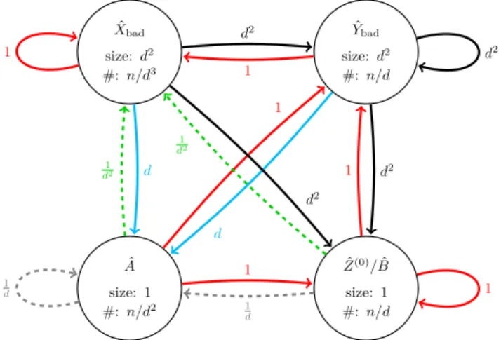
The weighted meta-graph in Figure 1 summarizes the situation after round 2. Each vertex in the meta-graph corresponds to one (or two) of the five classes of unstable vertices (we depict ˆZ(0) and ˆB as one vertex in all our figures because they evolve identically). The weights on the edges in the meta-graph are guided by the following idea. Assume that a vertex is, say, in an ˆXbad-structure, and assume pessimistically that its label can take over arbitrary parts of this structure. Then the weights of the arrows going out from ˆXbadare (an upper bound for) the expected number of structures of other types that the label sees (and thus, can potentially take over). If we pessimistically assume that it also takes over these new structures, then the weights of the outgoing edges in the meta-graph also gives a bound on the expected number of structures that the label can see form there, and so on. Thus if for each walk in the meta-graph we multiply the weights along a walk, and then sum these products over all walks in the meta-graph, then we obtain an a bound for the expected number of structures that the label can take over.

ˆ Ybad size:d2 #:n/d d2 ˆ Xbad size:d2 #:n/d3 1 d2 1 ˆ A size: 1 #:n/d2 1 d 1 d 1 d2 d ˆ Z(0)_/_Bˆ size: 1 #:n/d 1 1 d2 1 d2 d2 1 d 1

Figure 1 Meta-graph after round 2. The first value in a node S indicates the size of a structureS, the second value indicates number of vertices (counted with multiplicity) in structures of typeS. The weightx of a meta-edge from node S to node T indicates that from a random

S-structureS0there are in expectation at mostxedges toT-structures (not counting edges within S0 ifS=T). The same bound is also valid ifS0 is not random among allS-structures, but rather a random neighbour of aT0-structure, for any typeT0 that appears in the meta-graph. All values are upper bounds and suppress any polylog(d) factors.

An important intermediate goal is to show that the graph G0 = (V0, E0) induced by unstable vertices from ˆV is scattered, i.e. that most vertices are in small components. To this end, we would like to have that for any walk in the meta-graph, the weights of the edges multiply up to something of size o(1). Then, if we start with a random vertex in V0, all paths inG0 containing this vertex are short, since its unstable structure is only connected to few other meta-vertices. Hence, the vertex has small probability to be in a large component. Unfortunately, after round 2 the meta-graph is still much too dense for our purpose.

Analysing theMax-LPAprocess further, we show that in the third round the number of unstable ˆZ(0) _{and ˆ}_B _{structures decreases by a factor of ˜}_O₍₁_/d_{). For the ˆ}_Y

bad structures, something even more dramatic happens: most of them scatter internally by round 5, in the

(11)

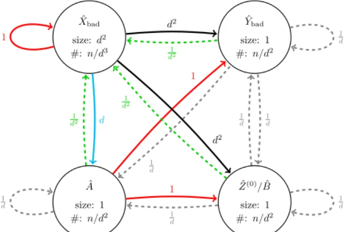
sense that if we choose a random vertex in a random ˆYbad structure, then the expected size of the component of this vertex within the ˆYbadstructure shrinks to ˜O(1). The analysis after round 2 becomes more tricky, since the structures lose their independence. For example, although the number of ˆZ(0)_/_Bˆ_{-structures decreases, the weight of the arrow ˆ}_A_→_Zˆ(0)_/_Bˆ does not decrease because neighbours of ˆA-vertices are biased towards remaining unstable. However, we can prove that some weights decrease as one would expect for random edges, namely for the edges between ˆYbad and ˆZ(0)/Bˆ, and the edges that go out of ˆYbad. The meta-graph after round 5 can be found in Figure 2.

ˆ Ybad size: 1 #:n/d2 1 d ˆ Xbad size:d2 #:n/d3 1 d2 1 d2 ˆ A size: 1 #:n/d2 1 d 1 1 d 1 d2 d ˆ Z(0)_/_Bˆ size: 1 #:n/d2 1 d 1 d 1 d 1 d2 d2 1 d 1

Figure 2Meta-graph after round 5. The first value in a nodeS indicates, given a random vertex

vin a random structureS0 of typeS, the size of the connected component ofvinduced by unstable vertices inS0. The weight of the edge fromS toT indicates how many edges intoT-structures there are in expectation from this connected component. Again, all bounds remain valid if we choosevas a random vertex as seen from structures of some typeT0. The second value in a nodeS indicates the number of unstable vertices in structures of typeS. All values are upper bounds and suppress any polylog(d) factors. Compared to round 2, only a ˜O(1/d)-fraction of the nodes in ˆYbadand in

ˆ

Z(0)_/_B_ˆ _{remain unstable. This decreases the weights from}_Y

badandZ/BintoYbadandZ/B by a factor of 1/d, but not the weights from ˆXbador ˆAinto these sets, because the target nodes of these edges are biased towards remaining unstable. Moreover, the remaining ˆYbad-structures are scattered into connected components of expected size ˜O(1), which decreases the weights of all outgoing edges from ˆYbadby 1/d2. There are no cycles in which the weights multiply to strictly more than one, and every cycle with a product of one is a combination of the cycles ˆXbad→Xˆbad, ˆXbad↔Yˆbad and

ˆ

Xbad↔Zˆ(0)/Bˆ.

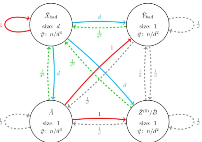
After round 5, there are still some cycles for which the weights do not multiply too(1), in particular the loop at ˆXbad and the cycles ˆXbad↔Zˆ(0)/Bˆ and ˆXbad↔Yˆbad. To deal with those, we use the fact that a typical leafv of an ˆXbad-structure sees neighbours in ˆYbad and in ˆZ(0)/Bˆ after round 2, but these do not see further unstable neighbours in round 3 and 4 with probability 1−O˜(1/d). In this case, we show that the leafvstabilizes by round 20, and we may decrease the weights from ˆXbad to ˆYbadand to ˆZ(0)/Bˆ accordingly (Figure 3). In the remaining meta-graph, all walks accumulate decreasing factors except for the loop for

ˆ

Xbad. However, since there are only ˜O(n/d4) vertices in ˆXbad structures, we can show that even the union of the connected components inG0 of all these structures has size ˜O(n/d4_). For all vertices outside of this union, a long path inG0 from such a vertex induces a long walk in the meta-graph, which is unlikely. Thus almost all vertices are either among the

˜

O(n/d4_{) vertices of ˆ}_X

bad components, or are in components of diameter less thanK, for a suitable constantK. For the latter one, we show that they stabilise afterK further rounds if the vertices are not contained in any cycles of length at most 2K.

(12)

ˆ Ybad size: 1 #:n/d2 1 d ˆ Xbad size:d #:n/d4 1 d 1 d2 ˆ A size: 1 #:n/d3 1 d 1 1 d 1 d2 d ˆ Z(0)_/Bˆ size: 1 #:n/d2 1 d 1 d 1 d 1 d2 d 1 d 1

Figure 3Meta-graph after round 20. Values have the same meaning as in Figure 2. Compared to Figure 2, theXbad-structures have decreased by a 1/dfactor in component size and in the number of unstable vertices, and the number of outgoing edges from ˆXbadto ˆYbadand to ˆZ(0)/Bˆhas decreased by a factor of 1/d. The only remaining cycle in which the labels multiply to one is the loop at ˆXbad.

6 Finishing the proof

For the last part of the proof, we fix a label, and show that this label cannot take over the complete graph. We only give the proof under the following simplifying assumption, and defer the full proof to the journal version. More precisely, we will assume that the label is

`max, the maximum label, and after round 100 we change the labels of all unstable vertices and all vertices whose label appears in a cycle of length at most 200 to`max. This gives the label class of`max a considerable boost after round 100, but it also simplifies the setting. In particular, since every other vertexv is stable and not in a cycles of length at most 200, the definition of stable implies that all neighbours ofv have either the label ofv, the label`max, or other mutually distinct labels. Moreover, after round 100 they have at least one neighbour of the same label, so they can only change their label to`max. This remains true inductively, since if a vertexvloses its neighbours of the same label, then those neighbours change their label to`max, and thusv also changes its label to`max. Thus the only possible change in the remaining graph is that vertices change their label to`max.

Let us first estimate the number of vertices that have or receive label`maxafter round 100. There are at most Õ(n/d4_{) unstable vertices by Lemma 13. Moreover, at this point no label} class has swallowed more than its 100-neighbourhood, which has sizeO(d100) = Õ(n/d4) whp (Lemma 2). Consider some δ >0. By choosingε=ε(δ) sufficiently small, if follows from Lemma 4 that the number of vertices that are contained in cycles of length at most 200 isO(nδ_{). Since each label class has at most size}_O₍_d100_{), the number of vertices with labels} that appear in such cycles isO(d100_nδ_{) = ˜}_O₍_n/d4_{), if we choose}_δ _{sufficiently small. Thus} after round 100 the label class of`max has size Õ(n/d4). In the following, we will show that with high probability, the structure ofGn,p is such that no set of this size can take over all the stable vertices in the graph.

First we argue that in order to take over a certain set of stable verticesS from one of the stable trees, there needs to be a certain number of edges going fromS to the vertices holding label`max. LetT ⊆V be the set of vertices that initially (i.e., after the relabelings in round 100) have label`max, and denote for each `6=`max byV` the set of vertices with

(13)

label`at this time. Now fix some later point in time t. LetT0 ⊇T be the set of vertices with label`max at roundt, and for each`6=`max, letS`=V`∩T0 be the set of vertices with label`that have been taken over by`max by roundt. Then we claim that

e(T0\T, T) +e(T0\T)≥ |T0\T|+ X `∈L,`6=`max

(e(S`, V`\S`) +e(S`)). (1)

To prove (1), let us assume thatv1, v2, . . . , vk is the order in which the vertices ofT0\T acquire the label`max, where we break ties arbitrarily. For an indexi≤k, let`i be the label ofvi and letTi:=T∪ {v1, . . . , vi−1}. Note that

e(vi, T0) =e(vi, Ti) +e(vi, T0\Ti).

Moreover, whenvi changes its label then all vertices inVì\Ti still have labelì. Hence,vi can only change its label ife(vi, Ti)≥e(vi, Vì\Ti) + 1, where the “+1” comes from the fact that the vertexv considers its own label as well when taking the majority. Hence,

e(vi, T0) =e(vi, Ti) +e(vi, T0\Ti) ≥e(vi, Vì\Ti) + 1 +e(vi, T 0_\_T i) = 1 +e(vi, Vì)−e(vi,{v1, . . . , vi−1} ∩Vì) +e(vi, T 0_\_T i).

Now we sum both sides over all 1 ≤ i ≤ k. Note that summing over e(vi, T0) yields

e(T0\T, T) + 2e(T0\T) since edges in T0\T are counted twice. Likewise, summing over

e(vi, V`i) yields

P

`6=`max(e(S`, V`\S`) + 2e(S`)), and summing overe(vi,{v1, . . . , vi−1} ∩V`i) yieldsP

`6=`maxe(S`). Finally, summing over e(vi, T

0_\_T

i) yields e(T0\T). Thus, summing and cancelinge(T0\T) yields

e(T0\T, T) +e(T0\T)≥k+ X `∈L,`6=`max

(e(S`, V`\S`) +e(S`)),

which implies (1) ask=|T0_\_T_|_.

Note that the terme(T0\T, T) +e(T0\T) on the left hand side counts the number of edges by which the label class of`max increases when it grows fromT toT0, while the term

e(S`, V`\S`) +e(S`) counts the number of edges withinV` which have at least one endpoint inS`. So basically (1) says that in order to recruitkvertices, the label class is “charged” at leastk+P

`6=`maxe(S`, V`\S`) +e(S`) edges. It is easy to check that the minimal ratio of

charged edges per recruited vertex is attained ifS`=V`is of size 2 for all`6=`max, in which case the ratio is 3/2 (three edges for two vertices).

Hence, in order to take over a set S of size kwe need at least 3k/2 edges inS∪V`max.

However, a sparseGn,pdoes not have sets of this density of order Θ(n/d3), as the following lemma shows.

ILemma 14(Lemma 4.2 in [11]). ConsiderGn,pwith1d=np=o(n). Letβ = 3₂−_{2 log(}1_d₎,

and sets= n

3d3. Then with high probability no set ofsvertices spans at least βsedges.

We may thus conclude the proof by contradiction as follows. Assume that `max would take over the graph. After round 100, it has sizes0= ˜O(n/d4), so at some later point the label class must have size s = n/(2d3_{). At this point, the number of edges in the label} class is at least 3

2(s−s0) = (1−O˜(1/d)) 3

2s≥βs, whereβ is as in Lemma 14. This is a contradiction to Lemma 14. Hence, the assumption must be wrong and`max cannot take over the graph. In fact, the proof shows that the label class of`max cannot grow to any size larger thanO(n/d3).

(14)

7 Conclusion

We have shown thatMax-LPAdoes not reach consensus onGn,pifp=O(n−1+ε). Consequently it fails to identify communities in planted network models. This disproves a conjecture by Kothapalli, Pemmarajum, and Sardeshmukh. Our result is obtained by combining a careful local analysis of the process with suitable global properties of the network.

For theMax-LPAprocess, it is natural to assume that there is some thresholdαsuch that for any smallδ >0 we have that forp= Ω(n−α+δ_{) the}

Max-LPAprocess reaches consensus onGn,pwith high probability, while forp=O(n−α−δ) it does not reach consensus with high probability. Assuming such anαexists, it follows from our result thatα≤1−ε; from [17] we know thatα≥1/4.

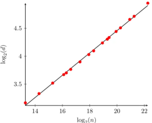
We conducted some experiments, which seem to suggest α= 4/5. Our experimental data was obtained by doing a binary search where in every step we ran the algorithm on 32 independentGn,p. If the majority of the runs converged with a unique label (modulo isolated vertices) then we decreased the value of pfor the following run, otherwise we increased it. We stopped when the change in the probability was small enough. To visualize the data we plot it on a log-log-scale, with basis 2 for the log. In this setting the exponent becomes a linear factor. We computed a linear regression of the log-log-data (i.e., the line which minimizes the sum of the square-distances of the log-log data points), and obtained the line log₂(d) = 0.19964 log₂(n) + 0.4652. Since the leading constant is very close to 0.2, this suggests that the correct threshold might bed= Θ(n1/5_{) and thus}_p_{= Θ(}_n−4/5_).

14 16 18 20 22 3.5 4 4.5 log2(n) log 2 ( d )

Figure 4Our experimental data with a linear regression. We plot an experimental evaluation of the thresholddsuch that theMax-LPAconverges in 50% of the cases with a unique label, on a log-log scale. The experimental data is extremely well described by a line with slope≈0.2, suggesting that the threshold satisfiesd= Θ(n1/5).

References

1 Michael J Barber and John W Clark. Detecting network communities by propagating labels under constraints. Physical Review E, 80(2):026129, 2009.

2 Luca Becchetti, Andrea Clementi, Emanuele Natale, Francesco Pasquale, Riccardo Silvestri, and Luca Trevisan. Simple dynamics for plurality consensus.Distributed Computing, 30(4):293– 306, 2017.

3 Luca Becchetti, Andrea Clementi, Emanuele Natale, Francesco Pasquale, and Luca Trevisan. Stabilizing consensus with many opinions. In Proceedings of the twenty-seventh annual

ACM-SIAM symposium on Discrete algorithms, pages 620–635. SIAM, 2016.

4 Punam Bedi and Chhavi Sharma. Community detection in social networks.Wiley

(15)

5 Petra Berenbrink, Andrea Clementi, Robert Elsässer, Peter Kling, Frederik Mallmann-Trenn, and Emanuele Natale. Ignore or comply? on breaking symmetry in consensus. arXiv preprint, 2017. arXiv:1702.04921.

6 Andrea Clementi, Miriam Di Ianni, Giorgio Gambosi, Emanuele Natale, and Riccardo Silvestri. Distributed Community Detection in Dynamic Graphs. Theor. Comput. Sci., 584(C):19–41, June 2015. doi:10.1016/j.tcs.2014.11.026.

7 Colin Cooper, Tomasz Radzik, Nicolás Rivera, and Takeharu Shiraga. Fast plurality consensus in regular expanders. arXiv preprint, 2016. arXiv:1605.08403.

8 Gennaro Cordasco and Luisa Gargano. Label propagation algorithm: a semi-synchronous approach. International Journal of Social Network Mining, 1(1):3–26, 2012.

9 Emilio Cruciani, Emanuele Natale, and Giacomo Scornavacca. On the Metastability of Quadratic Majority Dynamics on Clustered Graphs and its Biological Implications. CoRR, abs/1805.01406, 2018. arXiv:1805.01406.

10 Robert Elsässer, Tom Friedetzky, Dominik Kaaser, Frederik Mallmann-Trenn, and Horst Trinker. Efficient k-party voting with two choices. ArXiv e-prints, 2016.

11 Uriel Feige, Michael Krivelevich, and Daniel Reichman. Contagious sets in random graphs.

The Annals of Applied Probability, 27(5):2675–2697, 2017.

12 Mohsen Ghaffari and Johannes Lengler. Nearly-tight analysis for 2-choice and 3-majority consensus dynamics. InProceedings of the 2018 ACM Symposium on Principles of Distributed

Computing, pages 305–313. ACM, 2018.

13 Mohsen Ghaffari and Merav Parter. A polylogarithmic gossip algorithm for plurality consensus.

InProceedings of the 2016 ACM Symposium on Principles of Distributed Computing, pages

117–126. ACM, 2016.

14 Steve Gregory. Finding overlapping communities in networks by label propagation. New Journal of Physics, 12(10):103018, 2010.

15 Steve Harenberg, Gonzalo Bello, L Gjeltema, Stephen Ranshous, Jitendra Harlalka, Ramona Seay, Kanchana Padmanabhan, and Nagiza Samatova. Community detection in large-scale networks: a survey and empirical evaluation. Wiley Interdisciplinary Reviews: Computational Statistics, 6(6):426–439, 2014.

16 S. Janson, T. Łuczak, and A. Rucinski. Random graphs. Wiley-Interscience Series in Discrete Mathematics and Optimization. Wiley-Interscience, New York, 2000.

17 Kishore Kothapalli, Sriram V. Pemmaraju, and Vivek Sardeshmukh. On the Analysis of a Label Propagation Algorithm for Community Detection. InDistributed Computing and Networking, pages 255–269, Berlin, Heidelberg, 2013. Springer Berlin Heidelberg.

18 Ian XY Leung, Pan Hui, Pietro Lio, and Jon Crowcroft. Towards real-time community detection in large networks. Physical Review E, 79(6):066107, 2009.

19 Elchanan Mossel and Omer Tamuz. Opinion exchange dynamics. Probability Surveys, 14:155– 204, 2017.

20 Svatopluk Poljak and Miroslav S˘ura. On periodical behaviour in societies with symmetric influences. Combinatorica, 3(1):119–121, 1983.

21 Usha Nandini Raghavan, Réka Albert, and Soundar Kumara. Near linear time algorithm to detect community structures in large-scale networks. Physical review E, 76(3):036106, 2007.

22 Douglas Brent West et al. Introduction to graph theory, volume 2. Prentice hall Upper Saddle River, 2001.

23 Zhao Yang, René Algesheimer, and Claudio J Tessone. A comparative analysis of community detection algorithms on artificial networks. Scientific Reports, 6:30750, 2016.