IDRC photo: N. McKee
P O V E R T Y &
E C O N O M I C P O L I C Y
R E S E A R C H N E T W O R K
P M M A W o r k i n g P a p e r
2 0 1 0 - 0 8
Free Primary Education in Kenya: An
Impact Evaluation Using Propensity
Score Methods
Milu Muyanga
John Olwande
Esther Mueni
Stella Wambugu
March 2010
Milu Muyanga, (Research Fellow, Tegemeo Institute, Egerton University, Kenya); [email protected]
John Olwande (Research Fellow, Tegemeo Institute and Postgraduate Student, Department of Agricultural Economics, Egerton University, Kenya) [email protected]
Esther Mueni, (Postgraduate Student, Institute of Open Learning, Kenyatta University, Kenya) [email protected]
Stella Wambugu, (Postgraduate Student, Department of Agricultural Economics, University of Nairobi, Kenya) [email protected]
Abstract
This paper attempts to evaluate the impact of the free primary education programme in Kenya, which is based on the premise that government intervention can lead to enhanced access to education especially by children from poor parental backgrounds. Primary education system in Kenya has been characterised by high wastage in form of low enrolment, high dropout rates, grade repetition as well as poor transition from primary to secondary schools. This scenario was attributed to high cost of primary education. To reverse these poor trends in educational achievements, the government initiated free primary education programme in January 2003. This paper therefore analyzes the impact of the FPE programme using panel data. Results indicate primary school enrolment rate has improved especially for children hailing from higher income categories; an indication that factors that prevent children from poor backgrounds from attending primary school go beyond the inability to pay school fees. Grade progression in primary schools has slightly dwindled. The results also indicate that there still exist constraints hindering children from poorer households from transiting to secondary school. The free primary education programme was found to be progressive, with the relatively poorer households drawing more benefits from the subsidy.
Key words: Primary education, Programme evaluation, Propensity score, benefit incidence analysis, Kenya
JEL Classifications: I20, I21, I22
We gratefully acknowledge financial and scientific support from the Poverty and Economic Policy (PEP) Research Network, which is financed by the Australian Agency for International Development (AusAID) and by the Government of Canada through the International Development Research Centre (IDRC) and the Canadian International Development Agency (CIDA). We acknowledge comments received from Pramila Krishnan of University of Cambridge (UK), Jane Mariara of University of Nairobi (Kenya), Veronica Amarante of Universidad de la Republica, Montevideo (Uruguay), John Ataguba of University of Cape Town (South Africa) and Jean Yves-Duclos and Abdelkrim Araar of Laval University (Canada). We also acknowledge comments received from our numerous anonymous reviewers.
1. Introduction
The government of Kenya has committed itself to expanding its state education system to enable greater participation. This has been in response to a number of concerns, the main one being the desire to combat ignorance, disease and poverty as outlined in the Sessional Paper No.10 of 1965 on African Socialism and its Application to Planning in Kenya (Republic of Kenya, 1965). Consequently, every Kenyan child has the right of access to basic welfare provisions, including education, and the government has the obligation to provide its citizens with the opportunity to take part in the country’s socio-economic and political development, and to attain a decent standard of living.
Free primary education (FPE) was first introduced in Kenya in the late 1970s. However, the programme was later abolished in 1988 under the Structural Adjustment Programs (SAPs) to ease the financial burden on the public education system. These meant that parents had to contribute more towards education of their children through a cost-sharing programme. Parents were responsible for buying school uniforms, textbooks and other instructional materials for their children, as well as constructing buildings and providing other equipment to schools. The government retained the role of recruiting and paying teachers for their services.
The cost-sharing system somewhat led to high wastage within the primary education system in the form of low enrolment, high dropouts, grade repetition, low completion and poor primary to secondary transition rates (Bedi et al., 2002 and Kimalu et al., 2001). The gross enrolment rate (GER) dropped from 115 percent in 1987 to 95 percent in 1990 and further to 91 percent in 2002 (Republic of Kenya, 1988, 1991 and 2003a). Primary school GER declined from 98 percent in 1989 to 89 percent in 2002, while secondary school enrolment rate dropped from 29 to 23 percent during the same period. The GER for girls remained relatively lower than that for boys. In 2001 for example, the primary school GER was recorded at 90 and 91 percent for girls and boys, respectively. This scenario was attributed to the high cost of education, which had a negative impact on access, retention, equity and quality (Republic of Kenya, 2001). It is imperative to note that these trends were observed despite Kenya being among the highest spenders on education in Sub-Saharan Africa (Vos et al., 2004). However, over 75 percent of the education budget was spent for paying teachers’ salaries.
To reverse poor trends in educational achievements, the government initiated a free primary education (FPE) programme beginning January 2003. This policy was congruent with the 2001Student’s Act that calls for affordability of and equitable access to education in Kenya. The Act states that the government should provide free and compulsory primary
education. The FPE policy was also in line with other international declarations such as The World Conference on Education for All (EFA), held in Jomtien, Thailand in 1990, which underscored the importance of basic education and recognized that the cost of schooling was a major stumbling block to universal primary education in Sub-Saharan Africa among poor households (UNESCO, 1990), and the Millennium Development Goals (MDG) in which the world leaders made the achievement of universal primary education by the year 2015 as one of the goals.
2. Free Primary Education Programme in Kenya
The free primary education programme in Kenya was reintroduced by the National Rainbow Coalition (NARC) government elected into office in December 2002. Top-level dynamic political initiatives triggered FPE implementation, driven by a social contract with the electorate (Avenstrup et al., 2004). There was little time for consultations with the stakeholders. The FPE’s thrust was an ‘equity and socio economic agenda’ essentially aimed at narrowing the gaps of inequality in the country (Republic of Kenya, 2004). The premise of the FPE programme was that the main barriers to schooling come from income constraints and direct schooling costs. Before the beginning of 2003, parents offset a significant proportion of operational and development costs averaging 35 percent of the total costs in primary schools (Republic of Kenya, 2003b), and were also responsible for supplying instructional materials to the schools. The FPE programme’s primary objective was to provide enrolment opportunities for those children who were out of primary school due to schooling cost constraints.
The programme, however, does not single out only the poor in its implementation. Its implementation involves capitation payment to all public primary schools amounting to KSh.1020 (about US$14.57) per child per annum, with the amount disbursed based on the number of pupils enrolled in each school. About 36 percent of the payment goes to a General Purpose Account, which is used for the wages of supporting staff, repairs and maintenance, utility bills, postage, and general expenses. The remaining 64 percent of the payment goes to an Instructional Materials Account, which is used to purchase instructional materials. The funds are strictly allocated to the two accounts. In addition, within each account the funds are set aside for various expenditure items, and transfers between the expenditure items are prohibited. The FPE programme funds are managed by School Management Committees (SMC) comprised of the following individuals and their designations:
Head teacher-chair person
The chair person of the parents teachers association (PTA)
Two parents (non-members of the PTA) elected by parents
One teacher each to represent each grade
The FPE programme does not require parents and communities to build new schools, but to refurbish and use existing facilities such as community and religious buildings. However, the SMCs have argued that the programme’s payment allocation for repairs and maintenance is not adequate (UNESCO, 2005). If parents wished to charge additional levies, school heads and committees would have to obtain approval from the Ministry of Education, Science and Technology. The request to charge any levy has to be sent to the District Education Board by the Area Education Officer, after a consensus among parents expressed through the Provincial Director of Education, a process that primary school heads consider bureaucratic and tedious.
The immediate effect of the FPE was an improvement in primary school enrolment. The GER increased from 92 percent in 2002 to 104 percent in 2003 of the school age population (Republic of Kenya, 2007). The enrolment of girls rose by 17 percent, from 3 million in 2002 to 3.5 million in 2003, while that of boys rose by 18 percent from 3.1 to 3.7 million in the same period. By 2006, total enrolment in primary schools was 7.63 million, up from 7.59 million in 2005. It is also important to note that some of the students enrolling were adults (Appendix 1).
The dramatic rise in enrolment rates in schools presented a number of challenges. There was overcrowding in classrooms as most schools did not have adequate classrooms to accommodate the large number of pupils that enrolled under the FPE (UNESCO, 2005). The pupil-teacher ratio increased from 35:1 in 2000 to 43:1 in 2004 (Republic of Kenya, 2006). In many schools, the classroom sizes, especially in the lower classes, rose from an average of 40 to 120 pupils, resulting in overburdened teachers. Some pupils were forced to study under trees or in the open. There were also shortages of desks, equipment, and supplies. The quality of education offered under these circumstances remains questionable.
Besides these logistical problems, another pertinent question lingers: is the programme sustainable? In the 2003/04 financial year, the government increased its education budget by 17 percent. The donor community, which received the FPE policy with high enthusiasm, was quick to support the initiative. A discussion with the Ministry of Education officials revealed that the World Bank gave a grant of KSh. 3.7 billion, while the British government – through the Department for International Development – gave KSh. 1.6 billion towards the program. Other donors included the Organization of Petroleum Exporting Countries (OPEC), the Swedish government, and UNICEF. This may mean that the current cost of education
would be unaffordable if the country was to rely solely on domestic sources of funds to finance education.
3. Justification and Objectives of the Study
Education is critical to breaking the cycle of poverty. For poor parents, the opportunity to obtain primary education for their offspring is the first empowering step in their long journey out of poverty (Holyfield, 2002). Missed schooling opportunities or poor performance in schools are `irreversible disinvestments' (Voth et al., 2000). Children born into poor families often have poor educational outcomes. Studies exist pointing at parental poverty as the main reason for poor performance in schools (Cross and Lewis, 1998; Glewwe and Jacoby, 1994 and Wambugu, 2002). However, poverty is not only about income; it is also about inequitable access to services, lack of opportunities, reduced outcomes, and reduced hopes and expectations. The poverty experienced by the youth is often linked to childhood multidimensional deprivation and parental poverty: that in one way or another, the ‘older’ generation is unable to provide the assets required by the ‘younger’ generation to prepare it to effectively meet challenges faced during their youth (Moore, 2004). Parental poverty has always been associated with escalating rates of school drop outs, as pupils from poor parental backgrounds go to school on empty stomachs and dressed in tatters, making it
difficult for them to concentrate on their lessons or participate in school activities (Center for Public Policy Priorities, 1999).
Government intervention can lead to enhanced access to education, effectively affording the younger generation from poor households an equitable chance to escape from poverty in the future. Several studies have been conducted elsewhere to evaluate the impact of educational programs on schooling outcomes. Shapiro et al., (2004) evaluated the effectiveness of a compensatory education program in Mexico in improving student test scores and lowering repetition and failure rates. Study results showed that the program improved short-term learning results for disadvantaged students, although the improvement varied by the subject of instruction and the demographic characteristics of students taught. A study by Raymond and Sadoulet (2003) assessed the effectiveness of educational grants in raising schooling attainment of poor children in Mexico’s rural areas. Results showed that the per grade gains in reducing drop outs combined for an additional half a year in total schooling.
Progressive impacts were found along three dimensions: degree of poverty, parents’ education and distance to school. The children of uneducated fathers living far from school gained twice as much as their counterparts with an educated father or residing close to a school. The authors concluded that the educational grants successfully closed the schooling
gap along the wealth dimension but fell short of achieving the same in the other dimensions of parents’ education and school distance.
Newman et al, (2002) evaluated the impact of small-scale rural infrastructure projects in health, water, and education in Bolivia using an experimental design and propensity score matching methods. Results indicated that although education projects improved school infrastructure, they had little impact on education outcomes. Interventions in health clinics, on the other hand, raised utilization rates and were associated with substantial declines in under-age-five mortality rates. Investments in small community water systems had no major impact on water quality until this was combined with community-level training, though they did increase the access to and the quantity of water.
Results from the above studies indicate that directing education expenditures to the poor holds a promise for breaking the inter-generational transmission of poverty. This study specifically analyses trends in key primary education outcome indicators (school enrolment rates, grade progression and transition from primary to secondary schools) before and after FPE implementation; identifies the correlates of these outcome indicators; and examines the pro-poorness of the FPE transfer. The thrust of the study is how government intervention can stem parental poverty and its effects from extending into the future generation through children’s low educational attainment. Results from this study will aid in perfecting the FPE programme design and the recently introduced subsidised secondary education programme.
4. Data and Variables
The analysis uses panel data of children in the school going age drawn from about 1500 rural households. The data was collected as part of the Tegemeo Agricultural Monitoring and Policy Analysis project between Tegemeo Institute (Egerton University, Kenya) and the Department of Agricultural, Food and Resources Economics (Michigan State University, USA). The households were interviewed before the FPE programme was introduced in 1997, 2000 and after the programme had been implemented, in 2004 and 2007. Being panel data, the same households were interviewed in these four waves. All the districts were classified into seven agro-regional zones, as these zones bring together areas with similar broad climatic conditions and thus, rural livelihoods. Using standard proportional sampling aided by the national census data, households were sampled for interviews. Administratively, the households span 24 districts, 39 divisions and 120 villages. The questionnaire used to elicit information remained relatively stable over the years.
While the interviews extracted comprehensive information on both economic and social indicators of the households in all the four waves, data on members’ schooling was only well captured in the 2000, 2004 and 2007 waves. Schooling information relates to the household
members’ number of years spent in school prior to the survey and whether children in the school going age were attending school in the past year before the survey. The data, however, did not discriminate between attendance in private and public schools. In most cases in Kenya, private schools are found in urban centres. We made a bold assumption that the schooling information provided by the households relates to public schooling. A summary of variables is presented in table 1.
To measure the impact of the FPE programme in Kenya, we construct three main outcome indicators: (i) primary school enrolment; (ii) primary school grade progression; and (iii) secondary school enrolment. The choice of these indicators was dictated by data availability.
Primary school enrolment is a dichotomous variable measuring whether a child in the school going age was in or out of school during the year of the survey. A child generally enters grade one of primary school at age six (6) and is expected to exit grade eight (8) of primary school at age 13. School enrolment was estimated for year 2000, 2004 and 2007. To estimate the FPE programme’s impact on school enrolment, we compare enrolment in the period before (2000) and after (2004 and 2007) the programme.
Primary school grade progression is the average time (in number of years) spent by a pupil in one grade over a period of time (between two survey periods). A pupil is expected to advance one grade every subsequent year. The normal progression through schooling in Kenya includes between one and three years of pre-primary school, followed by eight years of primary school, and then four years of secondary school. Progression was measured as a difference between grades achieved in 2000 and 2004 and between 2004 and 2007. A continuous grade progression variable (index) bound between 0GP1 was constructed.
If the index was 0, it meant perfect retardation: the child was not making progress at all. If the index was 1, it indicated perfect progression from one grade to the next without repetition. To estimate the programme’s impact on grade progression, we compare the average grade progression index of 2000_2004 and that of 2004_2007. It is assumed that since the FPE programme started in 2003, it had not made a significant difference in progression rates in 2004. While the incidence of an extra age among pupils could also be used to measure grade progression, in this case it was not appropriate since many over-age persons enrolled in public primary schools after FPE was implemented.
Secondary school enrolment is a dichotomous variable. It measures whether a child in the secondary school-going age was in or out of school during the year of the survey. Here we are concerned about children who had completed primary education and were in the secondary school-going age (14-18 years). The variable takes a value ‘1’ if a child who had
completed primary education had been enrolled in secondary school and value ‘0’ if otherwise. The main aim was to examine whether secondary school enrolment improved/declined with the FPE. This was meant to indicate whether primary-secondary school transition improved/declined with the FPE programme. It is important to note that there were no measures put in place in the FPE programme to boost transition rate, so that any effect of the programme on secondary school enrolment must be considered indirect.
The following variables were used as explanatory in programme impact modelling:
Child-level: Age of child; gender of child; the relationship to caregiver; and a child’s
health. On health, data on whether any household member had been chronically ill for more than three consecutive months in the last twelve months preceding the survey thus making it impossible for him/her to work or attend school was elicited.
Household-level: Age of household head; gender of the household head; household size; highest educational attainment of household head; health; dependency ratio (measured by dividing the number of individuals aged below 15 or above 64 by the number of individuals aged 15 to 64); distance to the nearest school; and per capita household income.
Spatial variables: indicate the region where the household is situated to control for regional inequalities in incomes and opportunities.
5. Methodology
Even though the main goal of this study is to assess whether the FPE programme in Kenya has had an ‘impact’ on primary schooling outcomes, we first start by identifying the correlates of primary schooling performance indicators. Next, we evaluate the FPE programme using propensity score matching methods, and finish with benefit incidence analysis of the programme.
5.1 Correlates of primary schooling performance indicators
To examine the correlates of primary schooling outcome, the following pooled model is estimated: i i i i i i
t
c
h
r
y
1
2
3
(1)where
y
i represents the outcome of interest (primary school enrolment rate, grade progression or secondary enrolment rate) variable for individuali
.t
i is a step dummy variable used to capture whether there was structural change with the FPE programme. Year 2004 is used as the reference year. To test whether there was intercept shift with theFPE programme we test the null hypothesis
0 against
0. The coefficient indicates whether there was an increase or decrease in the probability of enrolment for a given year relative to the base year (2000), controlling for other observable factors. However, it must be noted that this might not be the appropriate way to test for the programme impact owing to functional form imposition and endogeneity problems.c
i,h
i andr
i are vectors representing child-level, household-level and regional-level background characteristics, respectively, for memberi
. Coefficients on the other independent variables represent the relative impact of those variables on the probability of the outcome of interest.The estimation strategy of equation (1) depends on the nature of primary education outcome of interest. For dichotomous dependent variables, i.e. primary and secondary school enrolment rates, we use a probit model. The probit model with White’s heteroscedasticity-robust standard errors returns consistent parameter estimates (Wooldridge, 2002). Using OLS to estimate fractional dependent variables like primary school grade progression is unlikely to yield consistent parameter estimates. To estimate the grade progression model, we use the quasi-maximum likelihood estimation (QMLE) method proposed by Papke and Wooldridge (1996). This method yields robust estimators of the conditional mean parameters with satisfactory efficiency properties.
5.2 Propensity score matching methods
Evaluating program effectiveness without a randomized control is a frequent necessity in most public programmes. Analysts typically use statistical modelling to estimate program impact. In recent years, propensity score matching (PSM) has gained attention as a potential method for estimating the impact of public policy programmes in the absence of experimental evaluations (Rosenbaum and Rubin, 1983). PSM is a semi-parametric technique used to estimate the average treatment effect of a binary treatment on a continuous scalar outcome. Although the technique was developed in the 1980s (Rosenbaum and Rubin, 1983) and has its roots in a conceptual framework which dates back even further (Rubin, 1974), its use in programme evaluation only became established in the late 1990s (Dehijia and Wahba 1999; Smith and Todd, 2005; Heckman et al.1998; Agodini and Dynarski, 2001; Dehijia and Wahba, 2002; Trevino and Shapiro, 2004; Jalan and Glinskaya, 2005; Ravallion and Jalan, 2000; and Esquivel and Alejandra, 2006).
In order to estimate the FPE’s average treatment effect on the programme’s participants, we would ideally want to estimate the following:
)
1
|
(
)
1
|
(
1
0
E
Y
D
E
Y
D
ATT
i i (2)where ATT is the average effect of the programme on its participants, D = 1 when an individual i participates in the programme and D = 0 when an individual i does not participate
in the programme.
E
(
Y
i0|
D
1
)
is the outcome for theth
i
individual that would have been observed had the individual not participated in the programme, whileE
(
Y
i1|
D
1
)
is the actual outcome for thei
th individual participating in the programme. The challenge is that)
1
|
(
Y
0D
E
i cannot be observed, that is we cannot observe the outcome for thei
thindividual had the individual not participated in the programme. This creates a need for establishing a counterfactual of what can be observed. To approximate the counterfactual, we undertake propensity score matching.
We are interested in comparing the difference between
Y
0 and Y1 for the same individual, that is)
,
1
|
(
)
1
|
(
)
(
X
E
Y
1D
E
Y
0D
X
(3)where X is a multidimensional vector of characteristics that influences participation in the programme. The component
E
(
Y
0|
D
1
,
X
)
is impossible to observe. When)
,
0
|
(
Y
0D
X
E
is used to approximateE
(
Y
0|
D
1
,
X
)
we run a risk of bias selection. The mean selection bias which occurs because of the use of non participants to approximate participant outcomes conditional on X is given by:)
,
0
|
(
)
,
1
|
(
)
(
X
E
Y
0D
X
E
Y
0D
X
B
(4)The PSM relies on the key assumption that conditional on observable characteristics X, participation must be independent of outcomes, that is(Y1,Y0)D|X , (the conditional
independence assumption, or CIA). Ideally, one would match a participant with a non- participant using the entire dimension of X (simple matching). But matching on every covariate is difficult to implement when the set of covariates is large. To overcome this curse of dimensionality, propensity scores (P(X)) – the probabilities of participating that are conditional on X - are used. Rosenbaum and Rubin (1983) show that if matching on covariates is valid, so is matching on propensity score. This allows matching on a single index rather than on the multidimensional X vector.
Because the FPE programme is mandatory1, we focus on estimating the average treatment effect of the programme over time. The only untreated pool from which the comparison sample may be drawn is the eligible population from the period before the
programme implementation, to give a before-after design2. Bryson et al. (2002) and Friedlander and Robin (1995) discuss non-experimental evaluation strategies, especially with respect to comparing the behaviour of persons in a particular area covered by a policy change to the behaviour of individuals in the same area before the change in policy. They conclude that in practice, despite the strategies, there is an obvious shortcoming with regard to the inherent difficulty in controlling for changes over time; these strategies are often the only ones available to the analyst as a result of data limitations or opposition to randomized experiments on ethical grounds. The conditional independence assumption (CIA) now becomes (Y1,Y0)T |Xwhere (T) indicates the time period (T 1 period when the programme is implemented and T 0 period before programme implementation).
It should be noted that when evaluating voluntary programmes, the conditional independence assumption (CIA) implies that X needs to be chosen such that X is correlated with the decision to participate in the program and the outcome. For mandatory government programmes, there is no decision whether to participate and X might need to be chosen based on different criteria (Lee, 2006). Matching here is an attempt to eliminate period bias rather than self-selection bias. In this case, propensity score matching controls for differences in the profiles of the two groups (before and after) but will not automatically allow for programme effects to be differentiated from temporal effects. The propensity scores help in matching persons who are similar (that is, both before and after programme implementation) according to a set of some conditioning variables (X). It is important to note that in the special case of schooling, and moreover schooling performance, unobservable factors such as child ability may be important in conducting propensity score matching. Unavailability of data on such important but unobservable attributes might seem to invalidate the choice of our methodological strategy. However, the propensity score method is the only technique available to us in this case where experimental data is absent.
We performed the matching process in two steps. In the first step, we used a standard logistic regression to generate propensity scores for each observation in the treatment and the non-treatment samples. The choice of conditioning (explanatory) variables used in predicting propensity scores was informed by review of literature on determinants of primary education outcomes and data availability. In the second step, we conducted one-to-one matching without replacement3 (also referred to as ‘single nearest-neighbour matching
2
Exact control group is non-existent since the programme is implemented in all public primary schools throughout the country. Private schools normally attract enrolment from relatively well-off members of the society and thus could not be used as a control group.
3For nearest neighbour matching, literature suggests the use of non-replacement to reduce the bias
without replacement’ in the literature) type of propensity-score balancing4. Recent literature suggests that other methods of propensity-score matching might not make that much difference (Zhao, 2004 and Michalopoulos et al. 2004). This approach chooses for each treatment group member the comparison group member with the closest estimated propensity score. For each treatment group member (observations in 2004 and 2007 taken separately), the comparison group member (observation in 2000) was chosen as the one that had the closest estimated propensity score. If several comparison group members matched a given treatment group member equally well, then one group was chosen randomly. Comparison group members were dropped from the analysis if they were not a best match for any treatment group member.
Traditionally, applications of nearest neighbour matching do not impose any support condition (Smith and Todd, 2005). However, following recent advice from the literature, we imposed a common support by setting a trimming level of 2 percent (i.e. dropping observations at which the propensity score density is very low), the level that was used in Heckman, Ichimura and Todd (1997), Smith and Todd (2005) and Lee (2006). The difference in outcomes for each matched pair and the mean across all pairs represent the average effect of treatment on the treated. The advantage of the propensity score matching is that a model or structure does not need to be imposed.
5.3 FPE programme benefit incidence analysis
Education is understood to be a basic service that is essential in any fight against poverty. Government intervention in education should be seen to promote less inequality and reduced poverty (Manasan et al., 2007). To meet these objectives, the FPE programme in Kenya adopted broad targeting. The broad targeting approach does not target the poor directly as individuals; rather, the poor are reached by targeting services or commodities consumed heavily by the poor, such as primary education and primary health care.
Examining the extent to which the poorest strata benefit from the FPE programme in Kenya is imperative. In the literature, two broad approaches have been pursued to measure the value of government programmes to its beneficiaries. The first, based on Aaron and McGuire (1970), considers an individual's own valuation of a programme; that is, the demand, or virtual, price. The difficulties inherent in estimating these prices led to the development of a less demanding approach known as benefit incidence analysis. Benefit incidence combines the cost of providing public services with information on their use to
better potential match. However, Zhao (2004) has shown that in practice, the difference between the two approaches is often small.
4
Matching was performed using PSMATCH2 STATA routine developed by Leuven, E. and B. Sianesi (2003).
show how the benefits of government spending are distributed across the population (van de Walle, 2003 and Castro-Leal, et al., 1997).
Though there are many ways to approach benefit incidence, a fairly standard method has emerged, mainly based on the work of Demery (1997), van de Walle and Nead (1995) and Selden and Wasylenko (1992). This method takes ‘‘across the population’’ to mean ‘‘across the expenditure (or income) distribution’’ – an approach consistent with the overall concern about poverty. It then estimates the distribution of benefits based on some variant of the average participation rate in a public program among people in different expenditure (or income) brackets.
In this study, we are interested in a general description of the FPE programme beneficiaries in terms of which income group draws more benefits. Therefore, we examine the average benefit incidence of the FPE programme per capita transfers across income quintiles. Income quintiles are defined on the basis of household incomes (not including the FPE transfers) to examine among which group the FPE transfer is concentrated. Income quintiles are formed by ranking the sample by household per adult equivalent income in 2004 and 2007. Quintiles are defined with equal numbers of people in each. So the poorest quintile refers to the poorest 20 percent in terms of income per adult equivalent.
As mentioned earlier, the FPE programme comprises an allocation equivalent to Ksh. 1,020 (about US$14.57) per child per annum. The total transfer per quintile depends on the total number of primary school enrolment of children whose households fall into the respective income quintiles. If lowest income groups have more children attending primary school than households in the higher income groups, then the lower income groups receive a larger share of the benefits from government spending than the higher income groups. If this scenario prevails, then the FPE programme can be judged as pro-poor.
According to Demery (2000), the amount of the education subsidy (
X
j) that benefits groupj
is defined as
n i n i i j ij j i ij jS
E
E
E
S
E
X
1 1 (5)where
X
j is the benefit incidence of spending on a service (say education) to groupj
,E
ijenrolments at level
i
,S
i is the government’s net spending on education at leveli
, and (i i
E
S
) is the mean unit subsidy of an enrolment at education leveli
. The share of total education spending to groupj
(X
j ) is:
n i n i i ij i i ij je
s
S
S
E
E
X
1 1 (6)It can be seen that this depends on two major components: First,
e
ij’s which are the shares of the group in total service use (in this case, enrolments). These reflect household behaviour. Secondly, thes
i, that is, the shares of spending across the different types of service, reflects government behaviour.6. Results and Discussions
The study results are presented and discussed in this section. First, summary descriptive statistics on the data are presented. Next, correlates of primary schooling outcomes are shown followed by the FPE programme impact evaluation results using the propensity score matching technique. Results from FPE programme benefit incidence analysis conclude the section.
6.1. Summary descriptive statistics of the variables
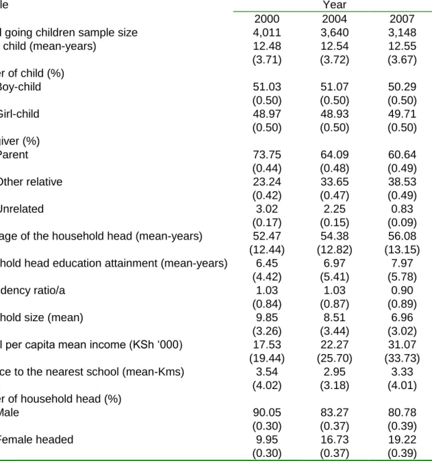
Overview of the summary statistics on the variables used in the analysis is presented in table 1. The number of school-going children in the sample declined from 4,011 in 2000 to 3,148 in 2007. The mean age in the contrary increased from 12.48 years in 2000 to 12.55 years in 2007. Among these children, approximately 51 percent were boys while 49 percent were girls in 2000. In 2007, the proportion of girls and boys stood at approximately 50 percent. The majority of school-going children were under the care of parents (74%), but this declined to 61 percent in 2007.
The mean age of the household head increased from 52 percent in 2000 to 56 percent in 2007. This increase is expected as these are panel households. Over 80 percent of the households were headed by males. However, the proportion of female-headed households nearly doubled between 2000 and 2007. The household head’s education attainment averaged between six and eight years of schooling. The mean dependency ratio declined from 1.03 in 2000 to 0.9 in 2007. The mean household size likewise declined from 10 to 7 between 2000 and 2007. Annual per capita mean income increased from KSh. 175,300 in 2000 to KSh. 310, 700 in 2007. The distance from the household to the nearest school declined from 3.5 km in 2000 to 3.3 km in 2007.
6.2. Correlates of the selected primary education performance indicators Primary school enrolment
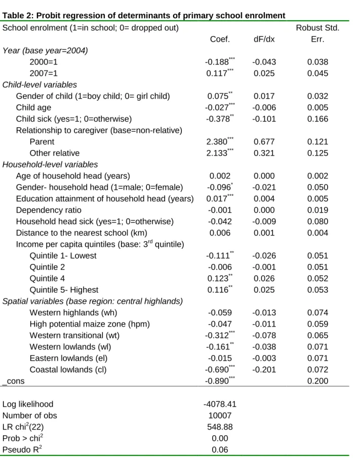
Results from a probit regression used to predict primary school enrolment is presented in table 2. Considering the likelihood ratio chi-square vis-à-vis the p-value, the model is statistically significant. The results also show that there was an increase in the probability of primary enrolment in the year 2007 relative to the base year (2004), controlling for other observable factors. Compared to the base year 2004, one year into the FPE programme, there was a lower probability of primary school enrolment in 2000.
At the child-level, the gender of the child, age, chronic sickness, and relationship to the care giver were found to be significant correlates of primary school enrolment. Compared to the boy-child, the girl-child has a higher probability of being out of school. As a child advances in age, the probability of being out of school increases. Perhaps this could be explained by the increased opportunity cost of being in school, as elder children are capable of getting jobs to augment household incomes. Children who were chronically ill had a lower probability of attending school. The results also indicate that children under the care of non-relatives are more likely to be out of school compared to children under the care of either their own parents or other relatives. Whereas chronic sickness by household head affected school enrolment negatively, the variable was not significant.
At the household level, gender and education level of the household head and household income are significant predictors of primary school enrolment. Children hailing from households headed by females have a higher chance of being in school. Children from households headed by persons with lower educational attainment had a higher probability of being out of school.
As expected, children from low income households are more likely to be out of school. Income quintiles are formed by ranking the sampled households based on per adult equivalent incomes. The first quintile represents the poorest 20 percent of households in terms of per adult equivalent income. Households belonging to quintile 3 are used as the reference group. On the other hand, children hailing from the first two wealthiest income quintiles are less likely to be out of school. Similarly, school enrolment varies across agro-ecological regions. The central highlands region was used as the base region. Children hailing from other regions are more likely to be out of school compared to children from the central highlands region. However, this relationship was only significant for the western transitional, western lowlands, and coastal lowland dummies.
Primary school grade progression
Next, results from QMLE of primary school grade progression for periods 2000-2004 (before FPE programme) and 2004-2007 (after the FPE programme) are presented (Table 3). The overall model is statistically significant. The coefficient of the programme dummy was negative and statistically significant at one percent level. This means that there was a decrease in grade progression in the period 2004-2007 relative to the base period 2000-2004, controlling for other observable factors.
While school grade progression is more or less a function of a child’s ability, there were some child- and household- level factors explaining grade progression. At the child level, age of the child and whether a child was sick for three months consecutively in the last twelve months preceding the survey were found to be significant predicators of grade progression. The age of the child positively influences grade progression. Also, children who had been sick for at least three months consecutively progressed less than children who had not been sick.
Educational attainment by the household head and household income were the most important predictors of grade progression at the household level. Children from households headed by members with high educational attainment progressed more than their counterparts from households headed by members with low educational attainment. While children from poorer households (20 percent poorest) progressed less than their counterparts in the higher income groups, the results are not statistically significant. Income quintile three is used as the base. However, children from the wealthiest quintile (20 percent wealthiest) were found less likely to repeat grades than children in income quintile three.
Just as in the case of primary school enrolment, primary school grade progression also varies across agro-ecological regions. The central highlands region is again used as the base region. Children from other regions are more likely to repeat grades compared to children from the central highlands region. This relationship is significant for the high potential maize zone, western transitional, western lowlands, and coastal lowland dummies.
Secondary school enrolment
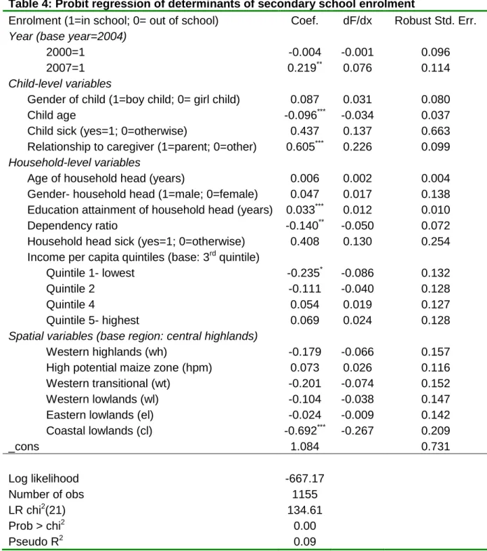
Results from probit regression of secondary school enrolment are presented in table 4. As mentioned earlier, the dependent variable takes the value 1 if a child that had finished primary school and still in the secondary school going age was enrolled in secondary school, and 0 if otherwise. Dummy variables were used to capture changes in transition rates in the years in consideration. Year 2004 is used as the base year. The results indicate that before the FPE program (year 2000), the probability of a child having completed primary education being in secondary school was lower compared to 2004. However, the finding was not
statistically significant. After the FPE programme was introduced, the scenario changed. The probability of a child being in secondary school after having completed primary education was higher in 2007. Among the most important child-level correlates of primary-secondary transition include age of child and relationship to the care-giver. As a child advances in age, the probability of not transitioning to secondary school increases. Children under the care of their parents have a higher probability of being in secondary school compared to their counterparts under the care of other relatives or non-relatives.
Educational attainment of household head, dependency ratio, and household income are the most significant predictors of primary to secondary school transition. Children from families headed by people with low educational attainment are less likely to enrol in secondary school compared to children from families headed by highly educated persons. This could be explained by the fact that highly educated parents are likely to be earning higher incomes and thus can afford the cost of secondary school education. Also, highly educated parents serve as role models to their offspring.
Children hailing from highly burdened households are less likely to continue with secondary education. Families with high dependency ratios are less likely to afford secondary school education. Similarly, the probability of children from relatively poor families proceeding with secondary education is lower compared to their counterparts from wealthier households. Children from the poorest 20 percent of households are less likely to continue with secondary education after completing primary education.
From the regional perspective, children hailing from most of the regions were less likely to proceed to secondary schools compared to those from the central highlands region. However, the relationship was only significant for the coastal lowlands dummy.
6.3. FPE programme impact evaluation using PSM results Primary school enrolment rates
The results from primary school enrolment analysis using propensity score matching methods are presented in table 5. In general, primary school enrolment has improved with the FPE programme introduction. Enrolment increased significantly from 82 percent in 2000, to 86 percent in 2004, to 89 percent in 2007; this is a seven percent increase between 2000 and 2007.
Generally, primary school enrolment increased after the introduction of the FPE programme across all income groups. Two very important points stand out from this analysis. First, higher income groups experienced a relatively higher increase in primary school enrolment in the period between 2000 and 2007. Secondly, the increase in primary
school enrolment for children belonging to the poorest 20 percent of households was not statistically significant. This finding probably indicates that factors that prevent children from poor backgrounds from attending primary school go beyond the inability to pay school fees. They could possibly include the opportunity cost of schooling and the ability to meet other basic needs such as clothing. A poor household may cherish free primary education, but rationally may be obliged to seek meeting immediate basic needs, thus prompting the household to send a child to work rather than to school.
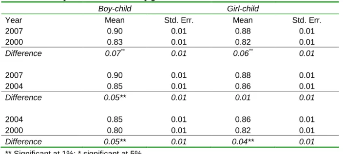
In 2000, primary school enrolment for the girl-child was relatively lower than that for the boy child; 82 percent and 83 percent, respectively (Table 6). In 2004, enrolment for the girl-child rose to 86 percent, overtaking that for the boy-girl-child (85 percent). But this was reversed in 2007, when the boy-child’s enrolment rose to 90 percent as against 88 percent for the girl-child. Difference of means tests for primary school enrolment between 2000 and 2004 and between 2000 and 2007 indicated that the increment in enrolment for both the boy- and the girl- child was statistically significant, signifying FPE’s role in enhancing primary school enrolment. Between 2004 and 2007, however, the difference in enrolment was significant only for the boy-child.
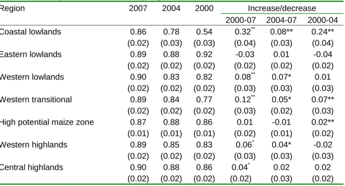
The increase in primary enrolment rates also varies by pupils’ region of origin (Table 7). While some regions experienced marked improvement in enrolment rates, in other regions primary enrolment declined. Five years after the introduction of FPE (2007), a dramatic increase in enrolment rates is witnessed across all regions except the Eastern lowlands. Between 2000 and 2007, the coastal lowlands experienced the largest and significant increase in enrolment of about 32 percentage points, followed by the Western transition with 12 percentage points. Compared to 2000, enrolment rates in 2004 and 2007 declined, albeit insignificantly, in the Eastern province by three and four percentage points respectively.
Primary school grade progression
Next, primary school grade progression trends are examined. As alluded to earlier, grade progression is measured as a difference between grades achieved between 2000 and 2004 and between 2004 and 2007. It is a continuous variable bound between 0 and 1. If the index is 0, it means no progression was made from one grade to the next (perfect retardation) during the period in focus. If the index is 1, then the child was advancing one grade each year without repetition during the period under consideration. To estimate the impact of FPE programme on grade progression, we compare the average grade progression index of 2000-2004 and that of 2004-2007.
Grade progression rates have slightly declined in the period under review (Table 8). The grade progression index dropped from 0.62 in the 2000-2004 period to 0.58 in the
2004-2007 period. The decline is statistically significant at one percent level. While appreciating that grade progression is more or less a function of a pupil’s ability, changes in grade progression after the introduction FPE programme vary across income groups (Table 9). The decline in grade progression rates was more pronounced and significant among children hailing from the 60 percent poorest households. The decline in grade progression among the 40 percent wealthiest households was not statistically significant.
Even though grade progression declined for both the boy- and girl- child after the introduction of FPE, grade progression for the boy-child remained relatively higher than that of the girl-child (Table 10). In the period 2000-2004, grade progression for both the boy- and girl- child stood at 0.62. However, in the FPE programme period (2004-2007) grade progression for the boy- and the girl- child significantly declined to 0.59 and 0.57, respectively.
Next, we analyse grade progression across agro-ecological zones (Table 11). After the introduction of FPE programme, primary grade progression declined in virtually all regions except in Central region where grade progression slightly increased, albeit insignificantly. The decline in grade progression was statistically significant only in Coastal lowlands, Eastern lowlands and High potential maize zone.
Secondary school enrolment
The success of education in stopping intergenerational poverty transfer hinges on primary graduates proceeding to secondary schools. First, we look at general cohort transition rates from the panel data. From the cohort that was in primary school in the 2000 survey and was expected to have joined secondary schools in 2004, only 37 percent transitioned. Similarly, only 33 percent of the cohort that was in primary school in 2004 and was expected to have proceeded to secondary school in 2007 actually did so. Therefore, only about one child out of every three children finishing primary education proceeds to secondary school, both before and after the introduction of the FPE period.
While transition rates among children from different household income levels were on average one-to-three (one child joining secondary education for every three children completing primary education), transition rates for children from poorer families have worsened after the FPE programme was introduced; out of every four children completing primary education, only one transitions to secondary school among the children hailing from the poorest 20 percent of households. Transition ratios of children from the wealthiest 20 percent of households were one for every three children finishing primary education.
The results from secondary school enrolment analysis using propensity score matching methods are presented in table 12. Generally, secondary school enrolment improved
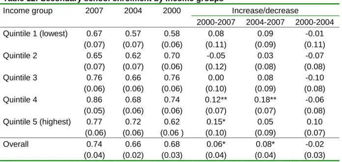
between 2000 and 2007. Enrolment rates increased from a mean of 68 percent in 2000 to 74 percent in 2007. However, a test of significance in the difference of the two means was only significant at the 10 percent level. Between 2000 and 2004, the enrolment rate declined from 68 percent to 66 percent. This decline was not significant, however. In relation to household income levels, results indicate that children from wealthier households had higher enrolment rates. Secondary enrolment rate for the children from the 20 percent poorest households was 58 percent while that for their counterparts from the 20 percent wealthiest households stood at 62 percent in 2000. In 2004, one year into the FPE programme, the enrolment for the children from the wealthiest group increased by seven percentage points to 72 percent. This improvement in enrolment was, however, not significant.
On the other hand, enrolment rates among children from the poorest income group declined, albeit insignificantly, by one percentage point to 57 percent. Between 2000 and 2007, secondary school enrolment rate for the two wealthiest income groups improved significantly. For the other income groups the change was not significant. These results indicate that there still exist constraints hindering children from poorer households from transitioning to secondary school after primary education.
There exist gender disparities in secondary enrolment rates (Table 13). The secondary school enrolment for the girl-child was relatively higher compared to that of the boy-child in 2000 - 67 percent and 65 percent, respectively. In 2004, the enrolment for the boy-child increased to 68 percent while that for the girl-child declined to 63 percent. These changes were, however, not significant. Comparing 2000 and 2007, secondary school enrolment rate for the boy-child rose by 19 percentage points to 84 percent. This increment was statistically significant at the five percent level. On the other hand, secondary school enrolment for the girl-child between the two periods slightly declined by one percentage point to 66 percent. However, the decline was not statistically significant.
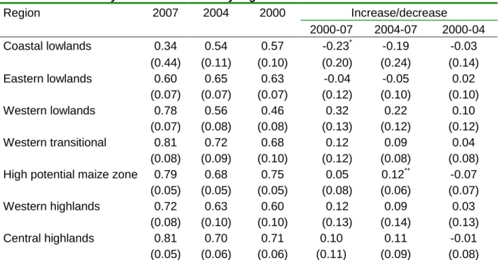
Secondary school enrolment rates also vary across regions (Table 14). In 2000, the High Potential Maize zone led in secondary school enrolment (75%). Western lowlands and highlands had the least secondary school enrolment rates (10%). In 2004 and 2007, while some regions experienced improvement in enrolment rates, others witnessed declines. Secondary school enrolment decreased significantly in the Coastal lowlands region by 23 percentage points between 2000 and 2007. In the High Potential Maize zone, the enrolment rate significantly improved by 12 percentage points between 2004 and 2007. The changes in enrolment in the other regions were not statistically significant.
6.4. Benefit incidence analysis results
Table 15 presents the distribution of primary school enrolment using income quintiles. The results are presented for 2004 and 2007. The first column in each year presents sample results while the second presents the population results. It should be noted that during sample selection, sampling weights were not taken into consideration. Nevertheless, an effort was made to construct probability weights to represent the probability that a case was selected into the sample from a population. These weights are calculated by taking the inverse of the sampling fraction. It can be observed from the results that immediately after the FPE programme introduction in 2004, the households in the second and the third quintiles had relatively more children enrolled in primary school compared to households in the first (20% poorest) and fifth (20% wealthiest) households. However, in 2007 there was a substantial shift in distribution of primary school enrolment across income quintiles. The primary school enrolment rates vary inversely with household income per adult equivalent. Poorer households have comparably more children attending primary school than their wealthier counterparts. Actually, the number of children enrolled in primary school from the households in the poorest 20 percent quintile is more than double the number from the wealthiest 20 percent income group.
As mentioned earlier, the FPE programme comprises a uniform allocation per enrolled child across the country. The allocation was KSh.1020 in 2004/05 and 2007/08 financial years. This implicitly means that benefit incidence is more or less a function of household behaviour rather than government behaviour.
In the first year after the introduction of FPE programme (2004), households in the second and third quintile captured most of the primary education subsidy (Table 16). However, with changes in enrolment across quintiles in 2007, the scenario changed. Government spending on FPE programme became pro-poor. The poorest 20 percent of households captured more than twice the government’s expenditure on FPE than their counterparts in the wealthiest 20 percent income group. This can be attributed to the fact that poorer households tend to have more children, and when schooling constraints are eased the same households are bound to have more children enrolled.
In figure 1, the estimates of children in the school-going age but are out of school, even though they have not completed primary education, are presented for 2004 and 2007. The results show that poorer households have more children out of school compared to the relatively wealthy households. Two important points stand out. First, the poorer households would benefit a lot more from the FPE programme if their children out of school could be enrolled. Second, as mentioned earlier, the reasons that scaled down enrolment rates in
primary school before the introduction of the FPE programme go beyond direct schooling costs.
7. Summary and conclusion
This study set out to evaluate the impact of the FPE programme in Kenya, to assess whether the programme is succeeding in reversing poor education trends. The FPE programme’s impact was evaluated using the propensity score matching method.
Results have shown that while primary and secondary school enrolment rates have significantly improved in the period after the introduction of the FPE program, grade progression has worsened. The improvement in primary school enrolment rates can largely be attributed to the FPE program and the primary education sensitization campaign that accompanied it. Increased secondary school enrolment could be attributed to the increase in primary school enrolment, as well as several secondary school bursary schemes that were introduced alongside the FPE program. Declining grade progression could indicate declining quality of primary education as a result of congestion, inadequate teachers and inadequate primary school infrastructure resulting from increased enrolment.
There is a need to improve primary school infrastructure and recruit more teachers. Secondary school enrolment rates remain low, especially among children hailing from poorer households and in some regions. This indicates a need for government intervention at the secondary school level. The recently introduced subsidised secondary education initiative is a step in the right direction and should be sustained.
Government spending on the FPE programme was found to be pro-poor. Despite lower enrolment rates, the poorest 20 percent of households capture more than twice the benefits of their counterparts in the wealthiest 20 percent income group, as poorer households tend to have more children. However, under this program, primary school enrolment rates increased most among children from the wealthier households. This finding suggests that the factors that prevent poorer children from attending primary school go beyond the inability to pay school fees. This indicates a need for pragmatic interventions to combat other factors beyond direct schooling costs that keep children from enrolling in school. Such interventions would definitely require an inquiry into the relevant hindrances to primary school enrolment, before these interventions can be instituted.
References
Abadie, A. and G.W. Imbens. 2006. Large Sample Properties of Matching Estimators For Average Treatment Effects. Econometrica, 74(1), pp. 235-267.
Agodini, R. and Dynarski, M. 2001. Are Experiments the Only Option? A Look at Dropout Prevention Programs, Mathematical Policy Research Inc., Princeton NJ.
Aaron, Henry, and Martin C. McGuire. 1970. Public Goods and Income Distribution.
Econometrica 38(6), pp. 907-20.
Avenstrup, R., Liang, X. and Nellemann, S. 2004. Reducing Poverty, Sustaining Growth. What Works, What Doesn’t, and Why? Case Study of Kenya, Lesotho, Malawi and Uganda: Universal Primary Education and Poverty Reduction. A Global Learning Process and Conference, Shanghai, May 25.27, 2004
Bryson, A., R. Dorsett and S. Purdon. 2002. The Use of Propensity Score Matching in the Evaluation of Active Labour Market Policies. Policy Studies Institute and National Centre for Social Research. Working Paper No. 4. United Kingdom
Bedi, Arjun, Paul Kimalu, Damiano Kulundu Manda and Nancy Nafula. 2002. The Decline in Primary School Enrolment in Kenya. Kenya Institute of Public Policy and Analysis (KIPPRA) Discussion Paper No. 14, Nairobi: KIPPRA.
Boccanfuso, Dorothée. 2005. Quasi-experimental methods: Propensity score matching (PSM). Presentation during the Workshop on the Assessment of the Poverty Impact of Public Programs.
Castro-Leal, Florencia, Julia Dayton and Lionel Demery. 1997. Public Social Spending in Africa: Do the Poor Benefit? Poverty and Social Policy Department, The World Bank, Washington D.C. (mimeo).
Center for Public Policy Priorities. 1999. Measuring Up: The State of Texas Education. February 26, 1999 No. 74 (http://www.cppp.org/products/policypages)
Cross, Toni G. and Lewis, George F. 1998. Early Manifestations of the Impact of Poverty on Education: The Expectant Parents' Hopes and Fears. Centre for Child Development Institute of Early Childhood, Macquarie University. Paper presented at the Australian Association for Research in Education Annual Conference, University of Adelaide, November 29-December 3, 1998
D’Agostino, R.B. 1998. Propensity Score Methods for Bias Reduction in the Comparison of a Treatment to a Non-randomized Control Group. Statistics in Medicine 17, 2265-2281) Dehijia, R. and Wahba, S. 1999. Causal Effects in Nonexperimental Studies: Re-evaluating
the Evaluation of Training Programs, Journal of American Statistical Association, 94(448), 1053-1062.
Dehijia, R. and Wahba, S. 2002. Propensity Score Matching for Non-Experimental Causal Studies, The Review of Economics and Statistics, 84(1): 151-161.
Demery, Lionel. 2000. Benefit Incidence: A Practitioner’s Guide. The World Bank. Washington, D.C.
Demery, L. 1997. Benefit Incidence Analysis. Poverty Reduction and Economic Management Network, Poverty Anchor. The World Bank. Washington D.C.
Esquivel, G. and Alejandra, H. 2006. Remittances and Poverty in Mexico: A Propensity Score Matching Approach. A Paper written under the auspices of Inter-American Development Bank (IADB).