Variable Selection when Confronted with Missing Data

(1)

VARIABLE SELECTION WHEN CONFRONTED

WITH MISSING DATA

by

Melissa L. Ziegler

B.S. Mathematics, Elizabethtown College, 2000

M.A. Statistics, University of Pittsburgh, 2002

Submitted to the Graduate

Faculty of Arts and Sciences in partial fulfillment

of the requirements for the degree of

Doctor of Philosophy

University of Pittsburgh

2006

(2)

UNIVERSITY OF PITTSBURGH FACULTY OF ARTS AND SCIENCES

This dissertation was presented by Melissa L. Ziegler It was defended on June 2, 2006 and approved by Satish Iyengar Leon J. Gleser Henry Block Douglas E. Williamson

(3)

VARIABLE SELECTION WHEN CONFRONTED WITH MISSING DATA Melissa L. Ziegler, PhD

University of Pittsburgh, 2006

Variable selection is a common problem in linear regression. Stepwise methods, such as forward selection, are popular and are easily available in most statistical packages. The models selected by these methods have a number of drawbacks: they are often unstable, with changes in the set of variable selected due to small changes in the data, and they provide upwardly biased regression coefficient estimates. Recently proposed methods, such as the lasso, provide accurate predictions via a parsimonious, interpretable model.

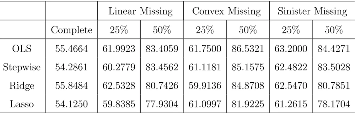
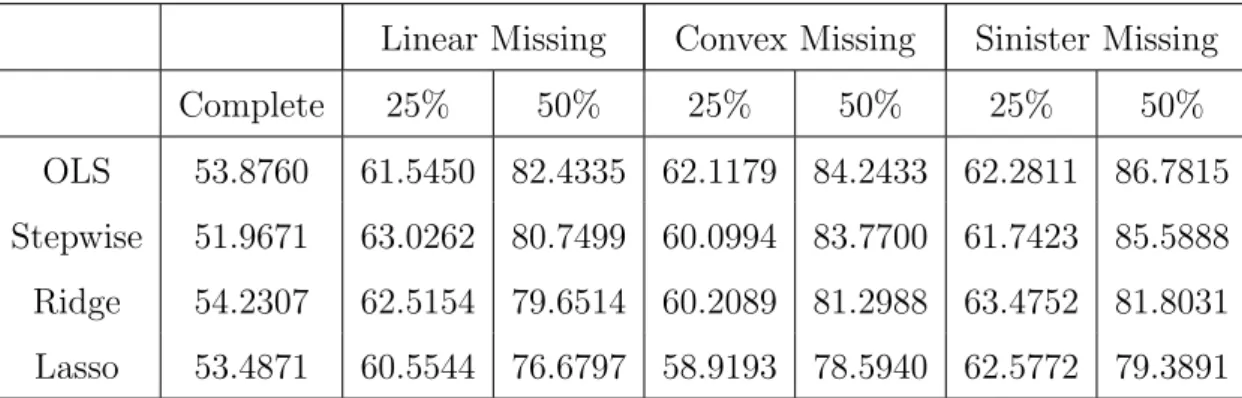
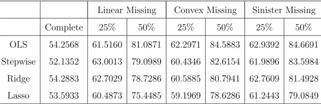
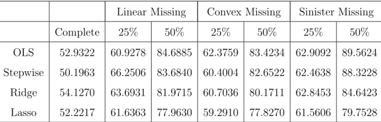
Missing data values are also a common problem, especially in longitudinal studies. One approach to account for missing data is multiple imputation. The simulation studies were conducted comparing the lasso to standard variable selection methods under different missing data conditions, including the percentage of missing values and the missing data mechanism. Under missing at random mechanisms, missing data were created at the 25 and 50 percent levels with two types of regression parameters, one containing large effects and one containing several small, but nonzero, effects. Five correlation structures were used in generating the data: independent, autoregressive with correlation 0.25 and 0.50, and equicorrelated again with correlation 0.25 and 0.50. Three different missing data mechanisms were used to create the missing data: linear, convex and sinister. These mechanisms

Least angle regression performed well under all conditions when the true regression pa-rameter vector contained large effects, with its dominance increasing as the correlation be-tween the predictor variables increased. This is consistent with complete data simulations studies suggesting the lasso performed poorly in situations where the true beta vector con-tained small, nonzero effects. When the true beta vector concon-tained small, nonzero effects,

(4)

the performance of the variable selection methods considered was situation dependent. Ordinary least squares had superior performance in terms confidence interval coverage under the independent correlation structure and with correlated data when the true regres-sion parameter vector consists of small, nonzero effects. A variety of methods performed well when the regression parameter vector consisted of large effects and the predictor variables were correlated depending on the missing data situation.

(5)

TABLE OF CONTENTS

1.0 OVERVIEW OF VARIABLE SELECTION METHODS . . . 1

1.1 Introduction . . . 1

1.2 Variable Selection . . . 1

1.3 Shrinkage Methods . . . 3

1.3.0.1 Ridge Regression . . . 4

1.3.0.2 Other Shrinkage Methods . . . 5

1.4 Combining Shrinkage and Selection . . . 6

1.4.1 Nonnegative Garrote . . . 6

1.4.2 Least Absolute Shrinkage and Selection Operator . . . 6

1.4.3 Least Angle Regression and Related Approaches . . . 7

1.4.4 Bridge Regression . . . 7

1.4.5 Elastic Net . . . 8

2.0 LEAST ABSOLUTE SHRINKAGE AND SELECTION OPERATOR 10 2.1 Lasso Basics . . . 10

2.1.1 Computational Algorithms . . . 10

2.1.1.1 Least Angle Regression Algorithm . . . 11

2.2 Comparison of Lasso to Other Methods . . . 11

2.3 Selection of Lasso Model . . . 13

2.4 Standard Errors for Lasso . . . 15

3.0 MISSING DATA METHODS . . . 17

3.1 Categorization of Missingness . . . 17

(6)

3.1.2 Missingness Mechanisms . . . 18 3.2 Overview of Methodology . . . 20 3.2.1 Deletion Methods . . . 20 3.2.2 Likelihood-Based Methods . . . 20 3.2.2.1 EM Algorithm . . . 21 3.2.3 Imputation . . . 22 3.2.3.1 Combination Rules . . . 23

3.2.4 Nonignorable Missingness Mechanisms . . . 24

3.3 Generating Imputations . . . 24

3.3.1 Assuming Normality . . . 25

3.3.2 Multiple Imputation by Chained Equations . . . 25

3.3.2.1 Gibbs Sampler . . . 26

3.3.2.2 MICE . . . 26

3.3.3 Included Variables . . . 28

4.0 SIMULATION STUDY OVERVIEW . . . 33

4.1 Simulation of Data . . . 33

4.1.1 Missing Data . . . 34

4.2 Comparison of Results . . . 35

5.0 RESULTS UNDER THE MISSING AT RANDOM ASSUMPTION . 36 5.1 Prediction Error. . . 36 5.1.1 Beta 1 - Independent . . . 37 5.1.2 Beta 1 - Autoregressive 0.25 . . . 38 5.1.3 Beta 1 - Autoregressive 0.50 . . . 39 5.1.4 Beta 1 - Equicorrelated 0.25 . . . 39 5.1.5 Beta 1 - Equicorrelated 0.50 . . . 41 5.1.6 Beta 2 - Independent . . . 41 5.1.7 Beta 2 - Autoregressive 0.25 . . . 43 5.1.8 Beta 2 - Autoregressive 0.50 . . . 44 5.1.9 Beta 2 - Equicorrelated 0.25 . . . 46 5.1.10 Beta 2 - Equicorrelated 0.50 . . . 47

(7)

5.1.11 Overall Results . . . 48

5.2 Confidence Interval Coverage . . . 50

5.2.1 Beta 1 - Independent . . . 52

5.2.2 Beta 1 - Equicorrelated 0.50 . . . 52

5.2.3 Beta 2 - Independent . . . 54

5.2.4 Beta 2 - Equicorrelated 0.50 . . . 55

5.2.5 Overall Results . . . 57

6.0 ANALYSIS OF MOTIVATING DATA . . . 58

6.1 Motivation . . . 58

6.1.1 Background . . . 59

6.2 Data Analysis . . . 60

6.2.1 Missing Data . . . 61

6.2.1.1 Amount of Missing Data. . . 61

6.2.1.2 Data Characteristics . . . 61

6.2.2 Motivating Data Results . . . 64

6.3 Conclusions . . . 70

7.0 FUTURE RESEARCH . . . 71

BIBLIOGRAPHY . . . 72

APPENDIX A. MAR PREDICTION ERROR TABLES- BETA 1 . . . 76

APPENDIX B. MAR PREDICTION ERROR TABLES - BETA 2 . . . 90

APPENDIX C. MAR PARAMETER ESTIMATES TABLES - N=50, P=5, BETA 1. . . 104

APPENDIX D. MAR PARAMETER ESTIMATES TABLES - N=50, P=5, BETA 2. . . 153

APPENDIX E. PSYCHOBIOLOGICAL MEASURES . . . 202

E.1 Growth Hormone Response to Stimulatory Tests . . . 202

E.2 Cortisol and Prolactin Response toL5HTP . . . 203

E.3 Cortisol and Adrenocorticotrophic Hormone Response toCRH . . . 204

E.4 Nighttime Cortisol and Growth Hormone Measures . . . 205

(8)

LIST OF TABLES

1 MAR, Beta 1, independent, n=50, p=5, MSE of Prediction . . . 37

2 MAR, Beta 1, autoregressive 0.25, n=50, p=5, MSE of Prediction . . . 38

4 MAR, Beta 1, equicorrelated 0.25, n=50, p=5, MSE of Prediction . . . 40

7 MAR, Beta 2, autoregressive 0.25, n=50, p=5 . . . 44

11 MAR - Incomplete Data versus Complete Data Standard Error Ratio. . . 51

12 Motivating Data Missing Data Percents . . . 63

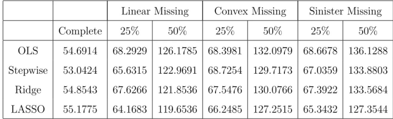
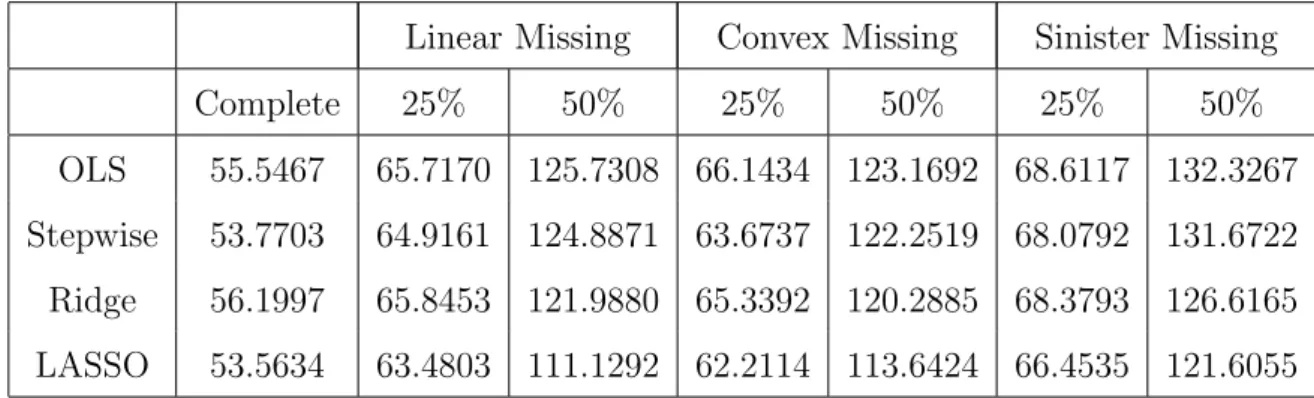
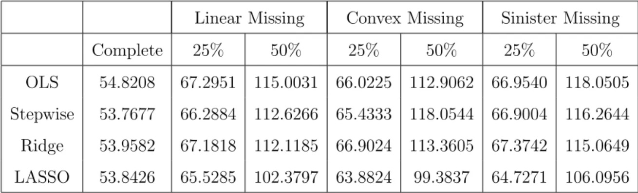
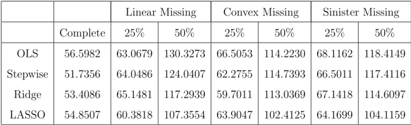
13 Ordinary Least Squares for motivating data . . . 66

14 Ridge regression results for motivating data . . . 67

15 Stepwise regression results for motivating data . . . 68

16 Lasso complete data results . . . 69

(9)

(10)

59 MAR, Beta 2,equicorrelated 0.25, n=100, p=10, MSE of Prediction . . . 99

61 MAR, Beta 2,equicorrelated 0.25, n=200, p=20, MSE of Prediction . . . 100

67 OLS - MAR, Beta 1, indep, n=50, p=5, Linear Missing at 25 percent . . . 105

68 Stepwise - MAR, Beta 1, indep, n=50, p=5, Linear Missing at 25 percent . . 106

69 Ridge - MAR, Beta 1, indep, n=50, p=5, Linear Missing at 25 percent . . . . 107

70 LASSO - MAR, Beta 1, indep, n=50, p=5, Linear Missing at 25 percent . . . 108

71 OLS - MAR, Beta 1, indep, n=50, p=5, Linear Missing at 50 percent . . . 109

72 Stepwise - MAR, Beta 1, indep, n=50, p=5, Linear Missing at 50 percent . . 110

73 Ridge - MAR, Beta 1, indep, n=50, p=5, Linear Missing at 50 percent . . . . 111

74 LASSO - MAR, Beta 1, indep, n=50, p=5, Linear Missing at 50 percent . . . 112

75 OLS - MAR, Beta 1, indep, n=50, p=5, Convex Missing at 25 percent . . . . 113

76 Stepwise - MAR, Beta 1, indep, n=50, p=5, Convex Missing at 25 percent . . 114

77 Ridge - MAR, Beta 1, indep, n=50, p=5, Convex Missing at 25 percent . . . 115

78 LASSO - MAR, Beta 1, indep, n=50, p=5, Convex Missing at 25 percent . . 116

79 OLS - MAR, Beta 1, indep, n=50, p=5, Convex Missing at 50 percent . . . . 117

80 Stepwise - MAR, Beta 1, indep, n=50, p=5, Convex Missing at 50 percent . . 118

81 Ridge - MAR, Beta 1, indep, n=50, p=5, Convex Missing at 50 percent . . . 119

(11)

83 OLS - MAR, Beta 1, indep, n=50, p=5, Sinister Missing at 25 percent . . . . 121 84 Stepwise - MAR, Beta 1, indep, n=50, p=5, Sinister Missing at 25 percent . . 122 85 Ridge - MAR, Beta 1, indep, n=50, p=5, Sinister Missing at 25 percent . . . 123 86 LASSO - MAR, Beta 1, indep, n=50, p=5, Sinister Missing at 25 percent . . 124 87 OLS - MAR, Beta 1, indep, n=50, p=5, Sinister Missing at 50 percent . . . . 125 88 Stepwise - MAR, Beta 1, indep, n=50, p=5, Sinister Missing at 50 percent . . 126 89 Ridge - MAR, Beta 1, indep, n=50, p=5, Sinister Missing at 50 percent . . . 127 90 LASSO - MAR, Beta 1, indep, n=50, p=5, Sinister Missing at 50 percent . . 128 91 OLS - MAR, Beta 1, equi 0.50, n=50, p=5, Linear Missing at 25 percent . . . 129 92 Stepwise - MAR, Beta 1, equi 0.50, n=50, p=5, Linear Missing at 25 percent 130 93 Ridge - MAR, Beta 1, equi 0.50, n=50, p=5, Linear Missing at 25 percent . . 131 94 LASSO - MAR, Beta 1, equi 0.50, n=50, p=5, Linear Missing at 25 percent . 132 95 OLS - MAR, Beta 1, equi 0.50, n=50, p=5, Linear Missing at 50 percent . . . 133 96 Stepwise - MAR, Beta 1, equi 0.50, n=50, p=5, Linear Missing at 50 percent 134 97 Ridge - MAR, Beta 1, equi 0.50, n=50, p=5, Linear Missing at 50 percent . . 135 98 LASSO - MAR, Beta 1, equi 0.50, n=50, p=5, Linear Missing at 50 percent . 136 99 OLS - MAR, Beta 1, equi 0.50, n=50, p=5, Convex Missing at 25 percent . . 137 100 Stepwise - MAR, Beta 1, equi 0.50, n=50, p=5, Convex Missing at 25 percent 138 101 Ridge - MAR, Beta 1, equi 0.50, n=50, p=5, Convex Missing at 25 percent . 139 102 LASSO - MAR, Beta 1, equi 0.50, n=50, p=5, Convex Missing at 25 percent 140 103 OLS - MAR, Beta 1, equi 0.50, n=50, p=5, Convex Missing at 50 percent . . 141 104 Stepwise - MAR, Beta 1, equi 0.50, n=50, p=5, Convex Missing at 50 percent 142 105 Ridge - MAR, Beta 1, equi 0.50, n=50, p=5, Convex Missing at 50 percent . 143 106 LASSO - MAR, Beta 1, equi 0.50, n=50, p=5, Convex Missing at 50 percent 144 107 OLS - MAR, Beta 1, equi 0.50, n=50, p=5, Sinister Missing at 25 percent . . 145 108 Stepwise - MAR, Beta 1, equi 0.50, n=50, p=5, Sinister Missing at 25 percent 146 109 Ridge - MAR, Beta 1, equi 0.50, n=50, p=5, Sinister Missing at 25 percent . 147 110 LASSO - MAR, Beta 1, equi 0.50, n=50, p=5, Sinister Missing at 25 percent 148 111 OLS - MAR, Beta 1, equi 0.50, n=50, p=5, Sinister Missing at 50 percent . . 149 112 Stepwise - MAR, Beta 1, equi 0.50, n=50, p=5, Sinister Missing at 50 percent 150

(12)

113 Ridge - MAR, Beta 1, equi 0.50, n=50, p=5, Sinister Missing at 50 percent . 151 114 LASSO - MAR, Beta 1, equi 0.50, n=50, p=5, Sinister Missing at 50 percent 152 115 OLS - MAR, Beta 2, indep, n=50, p=5, Linear Missing at 25 percent . . . 154 116 Stepwise - MAR, Beta 2, indep, n=50, p=5, Linear Missing at 25 percent . . 155 117 Ridge - MAR, Beta 2, indep, n=50, p=5, Linear Missing at 25 percent . . . . 156 118 LASSO - MAR, Beta 2, indep, n=50, p=5, Linear Missing at 25 percent . . . 157 119 OLS - MAR, Beta 2, indep, n=50, p=5, Linear Missing at 50 percent . . . 158 120 Stepwise - MAR, Beta 2, indep, n=50, p=5, Linear Missing at 50 percent . . 159 121 Ridge - MAR, Beta 2, indep, n=50, p=5, Linear Missing at 50 percent . . . . 160 122 LASSO - MAR, Beta 2, indep, n=50, p=5, Linear Missing at 50 percent . . . 161 123 OLS - MAR, Beta 2, indep, n=50, p=5, Convex Missing at 25 percent . . . . 162 124 Stepwise - MAR, Beta 2, indep, n=50, p=5, Convex Missing at 25 percent . . 163 125 Ridge - MAR, Beta 2, indep, n=50, p=5, Convex Missing at 25 percent . . . 164 126 LASSO - MAR, Beta 2, indep, n=50, p=5, Convex Missing at 25 percent . . 165 127 OLS - MAR, Beta 2, indep, n=50, p=5, Convex Missing at 50 percent . . . . 166 128 Stepwise - MAR, Beta 2, indep, n=50, p=5, Convex Missing at 50 percent . . 167 129 Ridge - MAR, Beta 2, indep, n=50, p=5, Convex Missing at 50 percent . . . 168 130 LASSO - MAR, Beta 2, indep, n=50, p=5, Convex Missing at 50 percent . . 169 131 OLS - MAR, Beta 2, indep, n=50, p=5, Sinister Missing at 25 percent . . . . 170 132 Stepwise - MAR, Beta 2, indep, n=50, p=5, Sinister Missing at 25 percent . . 171 133 Ridge - MAR, Beta 2, indep, n=50, p=5, Sinister Missing at 25 percent . . . 172 134 LASSO - MAR, Beta 2, indep, n=50, p=5, Sinister Missing at 25 percent . . 173 135 OLS - MAR, Beta 2, indep, n=50, p=5, Sinister Missing at 50 percent . . . . 174 136 Stepwise - MAR, Beta 2, indep, n=50, p=5, Sinister Missing at 50 percent . . 175 137 Ridge - MAR, Beta 2, indep, n=50, p=5, Sinister Missing at 50 percent . . . 176 138 LASSO - MAR, Beta 2, indep, n=50, p=5, Sinister Missing at 50 percent . . 177 139 OLS - MAR, Beta 2, equi 0.50, n=50, p=5, Linear Missing at 25 percent . . . 178 140 Stepwise - MAR, Beta 2, equi 0.50, n=50, p=5, Linear Missing at 25 percent 179 141 Ridge - MAR, Beta 2, equi 0.50, n=50, p=5, Linear Missing at 25 percent . . 180 142 LASSO - MAR, Beta 2, equi 0.50, n=50, p=5, Linear Missing at 25 percent . 181

(13)

143 OLS - MAR, Beta 2, equi 0.50, n=50, p=5, Linear Missing at 50 percent . . . 182 144 Stepwise - MAR, Beta 2, equi 0.50, n=50, p=5, Linear Missing at 50 percent 183 145 Ridge - MAR, Beta 2, equi 0.50, n=50, p=5, Linear Missing at 50 percent . . 184 146 LASSO - MAR, Beta 2, equi 0.50, n=50, p=5, Linear Missing at 50 percent . 185 147 OLS - MAR, Beta 2, equi 0.50, n=50, p=5, Convex Missing at 25 percent . . 186 148 Stepwise - MAR, Beta 2, equi 0.50, n=50, p=5, Convex Missing at 25 percent 187 149 Ridge - MAR, Beta 2, equi 0.50, n=50, p=5, Convex Missing at 25 percent . 188 150 LASSO - MAR, Beta 2, equi 0.50, n=50, p=5, Convex Missing at 25 percent 189 151 OLS - MAR, Beta 2, equi 0.50, n=50, p=5, Convex Missing at 50 percent . . 190 152 Stepwise - MAR, Beta 2, equi 0.50, n=50, p=5, Convex Missing at 50 percent 191 153 Ridge - MAR, Beta 2, equi 0.50, n=50, p=5, Convex Missing at 50 percent . 192 154 LASSO - MAR, Beta 2, equi 0.50, n=50, p=5, Convex Missing at 50 percent 193 155 OLS - MAR, Beta 2, equi 0.50, n=50, p=5, Sinister Missing at 25 percent . . 194 156 Stepwise - MAR, Beta 2, equi 0.50, n=50, p=5, Sinister Missing at 25 percent 195 157 Ridge - MAR, Beta 2, equi 0.50, n=50, p=5, Sinister Missing at 25 percent . 196 158 LASSO - MAR, Beta 2, equi 0.50, n=50, p=5, Sinister Missing at 25 percent 197 159 OLS - MAR, Beta 2, equi 0.50, n=50, p=5, Sinister Missing at 50 percent . . 198 160 Stepwise - MAR, Beta 2, equi 0.50, n=50, p=5, Sinister Missing at 50 percent 199 161 Ridge - MAR, Beta 2, equi 0.50, n=50, p=5, Sinister Missing at 50 percent . 200 162 LASSO - MAR, Beta 2, equi 0.50, n=50, p=5, Sinister Missing at 50 percent 201

(14)

LIST OF FIGURES

(15)

1.0 OVERVIEW OF VARIABLE SELECTION METHODS

1.1 INTRODUCTION

The goal of this research is to study and understand the properties of modern variable selection methods, to assess their performance in the presence of missing data, and ultimately to apply variable selection methodology to the motivating data set to find the covariates most closely related to, and predictive of, major depressive disorder (MDD). More details about the study and the data analysis are in chapter 6.

The following chapters will: (i) summarize the development of variable selection, with special attention paid to modern methods (Chapter1); (ii) provide a detailed analysis of the properties and implementation of the least absolute shrinkage and selection operator (lasso) (chapter 2); (iii) review missing data terminology and methods that will be applied in this research (chapter 3); (vi) detail the results of the simulation study that will examine the performance of variable selection methods when data are missing; (v) provide background on the psychobiology of depression in children and adolescents (chapter 6); and, finally (vi) highlight directions for future research (chapter7).

1.2 VARIABLE SELECTION

One of the most common model building problems is the variable selection problem [18]. In modeling the relationship between a response variable, Y, and a set of potential predictor variables, X1,· · · , Xp, what is desired is to select a subset of the possible predictors that explains the relationship withY, provides accurate predictions of future observations, and has

(16)

a simple, scientifically plausible interpretation. Many methods have been, and continue to be, developed to address this problem. This chapter will focus on variable selection methods, paying special attention to some of the more recent advances in this area. Additionally, the concept of shrinkage of parameter estimates will be introduced to provide a basis for understanding the most recent advances in variable selection methodology. These newer methods attempt to capitalize on the variance reduction provided by shrinkage methods to improve the performance of variable selection methods.

The history of selection methods is outlined in a 2000 review paper by George [18]. The development of these methods began in the 1960’s with methods designed to handle the linear regression problem which, due to its wide applicability, is still the focus of much of the new methodology. The early methods focused on reducing the rather imposing 2p _possible subsets of covariates to a manageable size using, for example, the residual sum of squares (RSS) to either identify the ‘best’ subset of a given size or to proceed in a stepwise manner to select covariates. Refinements of these methods add a dimensionality or complexity penalty to theRSS to penalize models with a large number of covariates. Examples of such penalties include Akaike’s Information Criterion (AIC) and the Bayesian Information Criterion (BIC). Advances in computing have expanded the use of variable selection methods to models such as nonlinear and generalized linear models. An overview and more detailed description of these methods can be found in Miller’s Subset Selection in Regression[29].

Stepwise variable selection methods are some of the most widely taught and implemented selection methods in regression. These methods are attractive because they provide an au-tomatic solution and thus are available in virtually every general statistics software package. Three types of stepwise methods are: forward selection, backward elimination and general stepwise regression (which combines forward selection and backward elimination). Forward selection starts with the model containing no predictors and adds one predictor at each step. Within a given step, the variable selected for inclusion in the model is that which minimizes the RSS. The process stops when some prespecified stopping criterion based on the amount of reduction in RSS between steps is met. On the other hand, backward elimination starts with the model containing all predictors under consideration and at each step the predictor that minimizes the RSS upon its removal. Again, the process continues until a prespecified

(17)

stopping criterion is met. Finally, general stepwise regression proceeds as in forward selec-tion, but with an added check at each step for covariates that can be removed from the model.

Stepwise selection methods have a number of drawbacks. Miller notes, “forward selection and backward elimination can fare arbitrarily badly in finding the best fitting subsets” [29]. The estimates of the regression coefficients of the selected variables are often too large in absolute value, leading to false conclusions about the actual importance of the corresponding predictors in the model. The value of R2 _{is often upwardly biased, overstating the accuracy} of the overall model fit. The estimates of the regression coefficients and the set of variables selected may be highly sensitive to small changes in the data. Selection bias and overfitting resulting from the use of the same data to select the model and to estimate the regression coefficients can be difficult to control [29]. Methods proposed to address one or more of these deficiencies will be considered in the next two sections (1.3, 1.4).

The following notation will be used in the description of the variable selection methods. Consider the usual regression model Y = β0_X₊_² _with _Y _the _n_×_{1 vector of responses,} _²

the n×1 vector of random errors, and X the n×p matrix of predictors with row vector xi the values for the ith _subject.

1.3 SHRINKAGE METHODS

Shrinkage estimators introduce a small amount of bias into a parameter estimate in an attempt to reduce its variance so that there is an overall reduction in the mean squared error (MSE). Some of the best known shrinkage methods are the James-Stein estimator and ridge regression.

The James-Stein result [23] demonstrates that the application of shrinkage can improve estimation under squared error loss. Let X ∼Np(ξ,Ip), that is, ξ = E(X) and

E(X −ξ)0_(X ₋_ξ_{) = I}

p. The goal is to estimate ξ, say by ˆξ, under squared error loss, L(ξ,ξˆ(X)) =kξ−ξˆk2_{. The usual estimator,} _ξ₀₍_X_{) =} _X_{, has expected}

(18)

an estimator, ξ1(X) = µ 1− p−2 ||X||2 ¶₊ X (1.1)

that has smaller expected loss thanξ0(X) for allξ, where (·)+ denotes the positive part [21].

1.3.0.1 Ridge Regression Ridge regression was proposed by Hoerl and Kennard [21] as a way to improve the estimation of regression parameters in the case where the predictor variables are highly correlated. The method introduces bias into the estimation process with the goal of reducing the overall mean square error. The ridge regression parameter estimates are given by

ˆ

βRR₍_k_{) = (X}0_X₊_k_I

p)−1X0Y (1.2) where k ≥ 0 and β = (β1,· · · , βp)0. Setting k equal to zero gives the usual ordinary least squares (OLS) estimators and for k >0 some bias is introduced into the estimates [21].

Hoerl and Kennard use the ridge trace, a plot constructed by simultaneously plotting each element of ˆβRR₍_k_{) versus}_k_{, to estimate the optimal value of}_k_{. The value of}_k_{is selected} at the initial point where the ˆβRR₍_k_{) estimates all appear to stabilize.}

The ridge regression estimates can also be expressed as a constrained minimization ˆ β = argminβ N X i=1 (yi−β0xi)2 subject to X j β2 j ≤t. (1.3)

where t ≥ 0 is a tuning parameter which controls the amount of shrinkage applied to the regression parameter estimates. By rewriting the ridge regression parameter estimates as

ˆ

βRR(k) = [Ip+k(X0X)−1]−1βˆOLS =ZβˆOLS, (1.4) the standard errors of the parameters can be obtained, as in linear regression, as

var( ˆβRR_{) = var(Z}_β_ˆOLS_{) =}_Z(X0_X)−1_X0_var(Y)X(X0_X)−1_Z0 _{= ˆ}_σ2_Z(X0_X)−1_Z0_. _(1.5)

This standard error estimate for ridge regression will be useful later to approximate the standard errors of parameter estimates in other variable selection methods.

(19)

1.3.0.2 Other Shrinkage Methods A variety of other shrinkage methods have been proposed for the regression situation. See Dempster, Schatzoff and Wermuth [15] for an extensive overview of past methods. Two of the more recent methods are highlighted in a comparison paper by Vach, Sauerbrei and Schumacher [43]. In the global shrinkage factor method, each of the regression coefficients is shrunk by a common shrinkage factorcwhich is estimated by cross-validation calibration. To obtain the cross-validated estimate ˆc, an OLS

regression of Y on X is performed with the ith _{observation removed resulting in ˆ}_βOLS (−i) for

i = 1,· · · , n. Using these estimated regression coefficients, predictions ˆY(−i) = ( ˆβ₍OLS₋_i))0Xi are computed. A simple linear regression of the orignal Y on the predictions ˆY(−i) is then performed and the resulting regression coefficient is used as the estimate ˆc. Note that the

Xi are assumed to be standardized so that

P

ixij/N = 0 and

P

ix2ij/N = 1 prior to any analyses. The shrunken regression coefficients are then obtained from the OLS estimators by ˆβ_jglobal = ˆcβˆOLS

j .

The second method extends the first by allowing parameter-wise shrinkage factors, that is, a different value of the shrinkage factor for each regression coefficient. Estimates of these parameter-wise shrinkage factors are again obtained by cross-validation calibration after standardizing the Xi. Parameter estimates can be obtained simply from the OLS estimates as ˆβP W

j = ˆcjβˆjOLS [43]. The parameterwise shrinkage method addresses one drawback of the global method, namely that it may shrink small coefficients too much. It is recommended that parameterwise shrinkage be applied subsequent to standard backward elimination due to the large number of parameters to be estimated if one starts with the full model. In this way, the pool of possible predictor variables is reduced first and then shrinkage is applied to provide some variance reduction [35]. This parameter-wise shrinkage can also be used directly as a technique for variable selection by setting coefficient estimates, ˆβj with negative shrinkage factors, that is ˆcj <0, to zero. [43].

Shrinkage methods provide some improvement overOLSin terms of mean square error of prediction, but generally do not reduce the number of predictors in the model. The variable selection methods discussed in section1.2 reduce the number of predictors, but may not do so in an optimal way. In the next section, the ideas of shrinkage and variable selection are combined to develop an improved variable selection method.

(20)

1.4 COMBINING SHRINKAGE AND SELECTION

Newer methods in variable selection have attempted to combine shrinkage with variable selection in regression to address some of the drawbacks of standard variable selection meth-ods. A number of methods which combine shrinkage and selection will be introduced here. The lasso, which will be the focus of this dissertation, will be introduced briefly here and described in more detail in Chapter 2.

1.4.1 Nonnegative Garrote

Breiman’s nonnegative garrote [8] is similar in form to parameter-wise shrinkage proposed by Sauerbrei [35] in that each parameter coefficient is shrunk by some factor ˆcj. Let ˆβOLS be the vector of OLS parameter estimates. Then the nonnegative garrote shrinkage factors, ˆ cj minimize X k Ã yn− X k ckβˆk OLS xkn !₂ subject to p X j=1 cj ≤t and cj >0, (1.6) wheret≥0 is the shrinkage threshold [8]. Variable selection is achieved when the coefficient associated with a particular variable is shrunk to zero, removing it from the model. One potential drawback of the nonnegative garrote is that the parameter estimates depend on both the sign and magnitude of the OLS estimates, causing this method to perform poorly in situations where the OLS estimates perform poorly, for example in situations involving high correlation among predictor variables [41]. The lasso estimates are not based on the

OLS estimates and in fact the lasso estimates may differ in sign from the OLS estimates.

1.4.2 Least Absolute Shrinkage and Selection Operator

The least absolute shrinkage and selection operator, or lasso, is a penalized regression method, where the L1 norm of the regression parameters is constrained below a tuning parameter t, which controls the amount of shrinkage applied and the number of variables selected for inclusion in the model [41]. As in the nonnegative garrote, variable selection

(21)

occurs when regression coefficients are shrunk to zero. The lasso parameter estimates are given by: ˆ β = arg min β N X i=1 (yi−βj0xi)2 subject to p X j=1 |βj| ≤t (1.7) where t ≥ 0 is a tuning parameter. As this method will be the focus of this dissertation, further details on the lasso are reserved for Chapter 2.

1.4.3 Least Angle Regression and Related Approaches

The least angle regression algorithm (LARS) presented by Efron, Hastie, Johnstone, and Tib-shirani [17] unites, under a common computational framework, three distinct, yet related, variable selection methodologies: forward stagewise linear regression, least angle regression, and the lasso. It is important to note the distinction between the least angle regression algo-rithm (LARS) and least angle regression as a model selection procedure. For each method, the algorithm proceeds in a stepwise manner through the pool of potential predictors, select-ing a predictor at each step based on the correlation with the current residual vector. The lasso formulation of the LARSalgorithm is of particular interest here because it provides an efficient algorithm for computing the lasso estimates needed for this research. Details of the modifications of the LARS algorithm needed to compute the lasso parameter estimates are in section 2.1.1.1.

1.4.4 Bridge Regression

Bridge regression [20] encompasses both ridge regression and the lasso as special cases by allowing the exponent in the constraint to vary. The bridge regression parameter estimates are given by ˆ β = arg min β N X i=1 (yi−βj0xi)2 subject to p X j=1 |βj|γ≤t (1.8) where the tuning parameter t ≥ 0 and the exponent γ ≥ 0 are estimated via generalized cross-validation. Ridge regression corresponds to γ = 2, and the lasso to γ = 1.

(22)

Fu [20] presents the results of a simulation study comparing bridge regression to OLS, the lasso, and ridge regression in the linear regression model. Each of the m= 50 data sets has n = 30 observations of p = 10 predictors. Each matrix has between-column pairwise correlationρm drawn from a uniform distribution on the interval (−1,1). The true vector of regression coefficients, βm, is drawn from the bridge prior,

πλ,γ(β) = γ 2−(1+1/γ)λ1/γ Γ(1/γ) exp µ −1 2 ¯ ¯ ¯ ¯_λ−β1/γ ¯ ¯ ¯ ¯ γ¶ . (1.9)

This prior distributions is a member of the class of elliptically contoured distributions [9]. As a special case, if we take γ = 2 in the bridge prior, the resulting distribution is normal with mean zero and variance λ−1_.

For fixed λ = 1, OLS, bridge regression, the lasso, and ridge regression are compared for γ = 1,1.5,2,3, and 4. For γ = 1 and 1.5, bridge regression and the lasso have a similar significant reduction in both MSE and PSE over OLS, whereas for γ = 2,3, and 4 both methods result in an increase in MSE over OLS. For all values of γ ridge regression has a moderate reduction inMSEand PSE, with similar amounts of reduction for allγ values. For

γ = 1 and 1.5 bridge regression and the lasso outperform ridge regression. These results agree with those of Tibshirani in that the lasso method outperformed ridge regression in those cases (γ = 1 and 1.5) where the true beta values were either zero or relatively large in absolute value, and was outperformed by ridge regression when the true beta values were small, but nonzero (γ = 2,3, and 4).

Because the performance of bridge regression and the lasso did not differ significantly for any value of γ and bridge regression provides a lesser degree of variable selection than the lasso for 1< γ < 2 and no variable selection for γ ≥2, this method will not be considered further in this research.

1.4.5 Elastic Net

A recently proposed generalization of the lasso and LARSis the elastic net [48]. The elastic net provides variable selection in the p > n case (where the lasso can select at most n

(23)

the lasso is dominated by ridge regression) and improves selection when groups of predictors are highly correlated (where the lasso typically simply selects one representative predictor from the group).

The basic idea of the elastic net is to combine the ridge regression and lasso penalties. In then¨aive elastic net, a convex combination ofL1- andL2- norms of the regression coefficients is constrained. The n¨aive elastic net parameter estimates are obtained via the constrained minimization

ˆ

βnEN = arg min β N X i=1 (yi−βj0xi)2 subject to (1−α) p X j=1 |βj|+α p X j=1 β2 j ≤t for some t. (1.10)

Zou and Hastie [48] present empirical evidence via both a real data example and a simulation study indicating that the n¨aive elastic net resulted in coefficient estimates that incurred ’double shrinkage’ leading to an increase in the bias without a corresponding decrease in the variance. They modified their original procedure by rescaling to avoiding overshrinking while preserving the advantageous properties the elastic net. The elastic net is given by

ˆ βEN = arg min β β 0 µ X0_X₊_λ 2I 1 +λ2 ¶ β−2y0_Xβ₊_λ 1 p X j=1 |βj| (1.11) Via their simulation study and real data example, Zou and Hastie [48] illustrate the properties of the elastic net and its performance relative to the lasso and ridge regression. The elastic net achieves better prediction error than both the lasso and ridge regression. The selection of groups of correlated predictors in the elastic net leads to the selection of larger models than the lasso. Whether the lasso or elastic net is a superior method depends on the goal of the analysis. If prediction is the goal, the lasso may be preferred because it selects only one representative predictor from highly correlated groups. However, if interpretation is the goal, the elastic net may be preferred because it will include all the predictors in a highly correlated group. Zou and Hastie propose the elastic net as a useful method in the analysis of microarray data, where the inclusion of highly correlated groups of predictors is preferred because these groups are biologically interesting.

(24)

2.0 LEAST ABSOLUTE SHRINKAGE AND SELECTION OPERATOR

2.1 LASSO BASICS

As described in section1.4.2, the least absolute shrinkage and selection operator(lasso) con-strains the L1 norm of the regression parameters. Variable selection occurs when regression coefficients are shrunk to zero.

Consider the linear regression situation with Y the n × 1 vector of responses yi and X the n×xp matrix of predictors, with row vector xi the values for the ith subject. The lasso assumes that either the observations are independent or that the yi are conditionally independent given the xij, where the xij have been standardized so that

P

ixij/n = 0 and

P

ix2ij/n = 1. In addition, the yi have been centered to have sample mean 0. Under these assumptions, the lasso estimates are given by:

ˆ β = arg min β n X i=1 (yi−βj0xi)2 subject to p X j=1 |βj| ≤t, (2.1) where t ≥ 0 is a tuning parameter which controls the amount of shrinkage applied to the parameter estimates and, therefore, the degree of variable selection [41].

2.1.1 Computational Algorithms

In order for the lasso to be applicable in practical situations, an easily implemented, efficient computational algorithm is needed. In the paper introducing the lasso method, Tibshirani [41] presented two different algorithms. The first is based on a method proposed by Lawson and Hansen [24] used to solve linear least squares problems under a number of general linear inequality constraints. The second method reformulates the lasso problem to construct

(25)

a quadratic programming problem with fewer constraints, but more variables, which can be solved by standard quadratic programming techniques. Many improvements of these algorithms have been suggested [30].

Osborne, Presnell, and Turlach [30] studied the lasso computations from the quadratic programming perspective, exploring the associated dual problem. The resulting algorithm was an improvement over those proposed by Tibshirani [41] and had the advantage of in-cluding the case where the number of predictors is larger than the number of observations. The exploration of the dual problem also provided improved estimates of the standard errors of the parameter estimates. Standard error estimation for the lasso parameter estimates will be discussed in detail in 2.4.

2.1.1.1 Least Angle Regression Algorithm The LARSalgorithm with a small mod-ification, provides efficient computation of the lasso parameter estimates. An additional constraint, sign( ˆβj) = sign(ˆcj), where ˆcj = x0j(y−βˆ0xj) i.e. the sign of any nonzero ˆβj in the model must agree with the sign of the current correlation is required [17] to obtain the lasso parameter estimates. The consequence of this restriction, in terms of computation, is that additional steps, compared with the unmodified LARS algorithm, may be required. In the regular LARS algorithm, once a covariate has entered the model, it cannot be re-moved, whereas with the lasso restriction in place, covariates can leave the model when the constraint above is violated. The LARS algorithm is easily implemented in the R software package version 2.2.1 in the lars library version 0.9-5 [32].

2.2 COMPARISON OF LASSO TO OTHER METHODS

The usefulness of the lasso method depends in large part on its performance in comparison with other variable selection methods and other types of parameter estimation. Simulation studies and real data examples have been used by several authors to illustrate the prop-erties of the lasso method and to compare its performance with other standard methods. Vach, Sauerbrei, and Schumacher [43] compared four of the more recently developed

(26)

vari-able selection methods: the global and parameterwise shrinkage factor methods (section 1.3), Breiman’s nonnegative garrote (section 1.4.1), and Tibshirani’s lasso (section 1.4.2) to backward elimination in ordinary least squares (OLS) in a simulation study. Four settings are considered in the simulation study, two involving independent covariates (A and B) and two involving pairwise correlated covariates (C and D). The correlated covariates condition is considered to examine the selection patterns for groups of correlated covariates. The true parameter values in each setting are:

βA_{= (0}_.₉_,₀_.₈_,₀_.₇_,₀_.₆_,₀_.₅_,₀_.₄_,₀_.₃_,₀_.₂_,₀_.₁_,₀_.₀₎0

βB_{= (0}_.₈_,₀_.₈_,₀_.₆_,₀_.₆_,₀_.₄_,₀_.₄_,₀_.₂_,₀_.₂_,₀_.₀_,₀_.₀₎0

βC _{= (0}_.₈_,₀_.₈_,₀_.₆_,₀_.₆_,₀_.₄_,₀_.₄_,₀_.₂_,₀_.₂_,₀_.₀_,₀_.₀₎0

βD_{= (0}_.₈_,₀_.₀_,₀_.₆_,₀_.₀_,₀_.₄_,₀_.₀_,₀_.₂_,₀_.₀_,₀_.₀_,₀_.₀₎0

The methods are compared in terms of complexity of the selected model, distribution of the shrinkage parameters, selection bias, prediction error, and the bias and variance of the parameter estimates. Model complexity is measured by both the inclusion frequency of each variable, that is the Pr{βˆj 6= 0}; and the average number of covariates selected. In settings

A,B, andC, in terms of both measures, the lasso selected the largest models, followed by the nonnegative garrote and then both types of shrinkage and backward elimination. In setting

D, the shrinkage methods select models that are larger than the nonnegative garrote. As in the other three settings, in setting D, the lasso selected the largest models and backward elimination selected the smallest models.

Selection bias is given by E[|βˆj| − |βj|

¯

¯_βˆ_j ₆_{= 0] for} _j _{= 1}_,_{· · ·}_{, p}_{. This definition of} selection bias differs from that typically used, for example Miller [29], in that the absolute values prevent under- and over-estimates from canceling out in small effects. [43] In terms of selection bias, the lasso is less biased in the case where the true parameter values are small, whereas the nonnegative garrote, parameterwise shrinkage, and backward elimination are least biased for large true parameter values. The authors conclude that overall the lasso performs well if one is aware of its propensity to underestimate large parameter values. The global shrinkage factor, while not a variable selection method, is useful in its reduction of average prediction error and the mean square error of the parameter estimates.

(27)

APE( ˆβ) = E[(Y∗₋_βˆ0_X∗₎2_]_, _{which can be expressed as} _APE ₌ _σ2 ₊_MSE _{where the mean} square error (MSE) is MSE( ˆβ) = E[ ˆβ0_(X∗₎₋_β_(X∗_)]2_{. Thus, comparisons based on} _MSE _of predictions are the same as those based on APE.

Taken together, the results of this simulation study do not clearly identify one method as best in all circumstances. The relative performance of the various methods depends not only on the true parameter values, as seen earlier, but also on the goal(s) of the analysis. For example, none of the methods considered performs well if parsimony is the most important criterion: they all resulted, on average, in larger models than backward elimination. Vach, Sauerbrei, and Schumacher [43] hypothesize that in order to achieve a reasonable level of parsimony, some sacrifice in terms of the other criteria must be made.

2.3 SELECTION OF LASSO MODEL

The LARSalgorithm provides a convenient, computationally efficient method for producing the full set of lasso coefficient estimates that avoids the computational burden of previously proposed lasso algorithms [41]. In fact, the entire set of lasso parameter estimates can be computed for an order of magnitude less computing time than previous methods [17]. However, because of the nature of the link between LARS, the forward stagewise method and the lasso, use of the LARS algorithm removes the automatic model selection provided by the direct use of the tuning parameter to control the amount of shrinkage and selection in the lasso.

In the LARSalgorithm, a Mallows’ Cp-type statistic is proposed for selecting the optimal model in LARS. An approximation of this statistic is given by

Cp(βˆ[k])∼= (ky−βˆ[k]Xk2)/(¯σ2)−n+ 2k, (2.2)

where ˆβ[k] _{is the vector of the} _k_-step _LARS _{parameter estimates and ¯}_σ2 _{is the residual} mean square error of regression on k variables. This Cp estimate applies only for the LARS selection method, not for the lasso or the forward stagewise method [17]. The proposed

(28)

many discussions ofLARSpaper [17]. In particular, the first discussant, Ishwaran, shows in a simulation study that the use ofCp can lead to models that are too large. He suggested that accounting for model uncertainty through model averaging may improve the performance of the Cp statistic. Stine also criticizes the Cp statistic and proposes the Sp statistic, another penalized residual sum of squares estimate, to be used instead. This statistic is given by

Sp =RSS(p) + ˆσ2 p X j=1 2j log µ j+ 4 j+ 2 ¶ , (2.3)

where p is the number of predictors in the current model and ˆσ2 _{is “an honest estimate of}

σ2_{” computed using the (conservative) estimated error variance from the model selected by} the standard forward selection method. Using Sp to select the model size resulted in the selection of a model that is smaller than that selected by Cp and has smaller residual mean square error.

Leng, Li and Wahba [25] found that under the minimum prediction error criterion,LARS

and the lasso are not consistent variable selection methods. A consistent variable selection method is one in which the probability of correctly identifying the set of important predictors tends to one as the sample size tends to infinity. Moreover, it is shown that the probability of selecting the correct model in LARS or the lasso is less than a constant not depending on the sample size. In simulation studies, the lasso method selected the exact true model with small probability between 10% and 30%. The authors are careful to point out that their criticisms are not with the LARSconcept; they question only the validity of the use of prediction error as a criterion for selecting the tuning parameter. Other criteria may provide consistent variable selection.

The use of a form of the BIC for model selection with the lasso is proposed by Zou, Hastie and Tibshirani [49]. The authors present a more careful examination of the degrees of freedom for the lasso than do Efron, Johnstone, Hastie and Tibshirani [17]. They prove the following for the lasso: “Starting at step 0, let mk be the index of the last model in the Lasso sequence containing k predictors. Then df( ˆβ[mk])∼=k.” This implies that the degrees

of freedom for the lasso estimates containing k nonzero coefficients, obtained bymk steps, is approximatelyk. Note that the number of steps could be larger than the number of nonzero coefficients because predictors that have entered can exit the lasso model in later steps.

(29)

Given this approximation for the degrees of freedom, selection methods based on Akaike’s Information Criterion (AIC) and the Bayesian Information Criterion (BIC) are derived for the lasso. Based on the properties ofAIC andBIC as described in section1.2 and supported by the results of their simulation study, Zou, Hastie and Tibshirani [49] recommend the use of

BIC in selecting the lasso model when variable selection is the primary goal. BICwas shown to select the exact correct model with higher probability than AIC which conservatively included additional covariates. In comparison with the Cp-type statistic suggested inLARS, the BIC criterion selected the same 7 covariates from among 10 predictors and a smaller 11 variable model compared with the Cp 15 variable model from among 64 predictors.

Recall that theLARSalgorithm produces the complete set of lasso parameter estimates, providing the ‘best’ model of each size (number of nonzero coefficients)kfor the computation cost of the fit of a single least squares regression model. A theorem proved by Zou, Hastie and Tibshirani shows that the optimal lasso model is among the models in the LARS algorithm output, thus we need only choose between them. Computation of the BIC based on the output of the LARS is simplified by the following result. Let β[mk] be the vector of lasso

parameter estimates at the mth _{step in the algorithm with} _k _{nonzero coefficients at a given} iteration. To find the optimal number of nonzero coefficients, we need only solve [49]

kopt = arg min k

ky−β[mk]0Xk2

nσ2 +

log(n)

n k. (2.4)

Because of the easy of implementation using the lasso estimates provided by the LARS

algorithm and the evidence pointing to the BIC as the ‘best’ stopping criterion proposed thus far, BIC for the lasso will be used to select final models in this research.

2.4 STANDARD ERRORS FOR LASSO

The usefulness of the lasso method in practice depends in part on the accuracy of the param-eter estimates. In order to perform significance testing for individual paramparam-eter estimates, estimation of the standard errors of the lasso parameter estimates will be required. A number of standard error estimates have been proposed in the literature.

(30)

Tibshirani [41] presents two standard error estimates: one based on bootstrap resam-pling, and a closed form expression using an approximation based on ridge regression. The standard error estimate based on bootstrap resampling. The second standard error esti-mate is developed by exploiting the connection between the lasso and ridge regression. This method has the undesirable property of giving the estimate zero for any regression coefficient that was shrunk to zero by the lasso. Improvements on these standard error estimates have been proposed by Osborne, Presnell and Turlach [30] (see equation 2.7).

Tibshirani’s estimate is

ˆ

var( ˆβlasso)T IBS = (X0X+αW−)−1X0X(X0X+αW−)−1σˆ2 (2.5) where ˆσ2 _{is an estimate of the error variance,} _W ₌ _diag₍_|_βˆlasso

j |) and α is chosen so that

P

j|βˆjlasso|=t. The improved estimate [30] is given by ˆ

var( ˆβlasso)OP T = (X0X+V)−1X0X(X0X+V)−1σˆ2 (2.6) where, again, ˆσ2 _{is an estimate of the error variance and} _V _{is a slightly more complicated} expression than W given by

V =X0 Ã 1 kβˆlassok1kX0r k∞ rr0 ! X (2.7)

where r = r( ˜β) = (Y−β˜0_{X) is the vector of residuals corresponding to} _β_{. The standard}

error estimate, ˆvar( ˆβlasso)OP T, presented by Osborne, Presnell and Turlach has been shown to be superior to that of Tibshirani and will be used in this research.

(31)

3.0 MISSING DATA METHODS

Almost all longitudinal data sets have missing data values, and the motivating data for this study is no exception. The goal of this research is to assess the performance of the variable selection methods described in chapters1and2in the presence of missing data. Major texts on missing data methods include Analysis of Incomplete Multivariate Data by J.L. Schafer [36] andStatistical Analysis with Missing Databy Roderick J.A. Little and Donald B. Rubin [26].

The following notation, taken from Little and Rubin [26], will be used in the discussion of missing data. LetY ={yij}denote annbykrectangular data set without missing values. Define themissing-data indicator matrix M = (mij), such that mij = 1 if yij is missing and

mij = 0 if yij is observed. The matrix M then describes the pattern of missing data.

3.1 CATEGORIZATION OF MISSINGNESS

Missing data are commonly classified based on two characteristics: the pattern of missing values and the missingness mechanism. Together, these classifications can indicate which method is appropriate for the missing values in a data set. Some methods are developed to be applied only with data that follow a specific pattern. For example, many methods are useful only in the case of a monotone missing data pattern. Other methods can be used with a general pattern of missingness, but some computational savings can be achieved if the data follow a special pattern.

(32)

3.1.1 Missing Data Patterns

Three broad categories of missing data patterns: monotone missingness, file matching and general missingness, are defined by Little and Rubin [26]. Consider a set of variables

y1,· · ·, yk observed on a set of individuals. A monotone missing data pattern is one in which the variables can be ordered in such a way that when yj is missing for a given indi-vidual the variables yj+1 through yk are also missing [37]. Subject attrition in longitudinal studies is one example of a monotone pattern of missing data. It is important to note that the covariates need not be collected over time for a monotone pattern of missing to exist. The file matching pattern of missingness occurs when two variables (or two sets of variables) are never jointly observed. Arbitrary missingness describes any pattern that cannot be classified as either monotone or file matching.

3.1.2 Missingness Mechanisms

The missingness mechanism attempts to answer, from a statistical perspective, the question of why data is missing. Meng [28] describes the missingness mechanism as the process that prevents us from observing the intended data. What is of central importance is the probabilistic relationship between the value that should have been observed (the intended data) and the fact that it was not observed. This relationship is defined statistically in terms of the conditional distribution of the missing data indicator matrix given the observed data. The three general types of missing data mechanisms defined by Little and Rubin [26] are missing completely at random (MCAR), missing at random (MAR), and not missing at random (NMAR). To characterize the distinctions between these categories, let the condi-tional distribution of the missing data mechanism M, given the data Y = (Yobs, Ymis) be denoted by f(M|Yobs, Ymis, φ), where φ denotes unknown parameters related to the missing data mechanism.

Missing completely at random is the case when nonresponse and the data values (both missing and observed) are unrelated; that is, nonresponse is unrelated to both the value that should have been observed and was not, and to the other values in the data set. Under the

(33)

data Y is given by

f(M|Yobs, Ymis, φ) = f(M|φ) for all Yobs, Ymis, φ. (3.1) TheMCAR assumption is often too strong to be plausible in practical situations [28], except in the case where data is missing by design [26]. An example of data missing by design is the double sampling method, often used in survey sampling, where the entire sample is asked one set of questions and only a preselected subsample of respondents is asked an additional set of questions.

A more plausible, but weaker assumption, is that the data is missing at random (MAR). Under the MAR mechanism, the missingness depends only on the observed components of the data, Yobs, not on the missing values, Ymis. That is,

f(M, Yobs, Ymis|, φ) =f(M|Yobs, φ) for all Ymis, φ. (3.2)

In other words, after other variables in the analysis have been controlled for, the missingness is unrelated to Ymis [1].

If, in addition to meeting the MAR assumption, the parameters governing the complete data model,θ, and those governing the missing data mechanism,φ, are distinct in the sense that the joint parameter space ofθandφis the Cartesian product of the parameter space ofθ

(Ωθ) and the parameter space ofφ(Ωφ), i.e., (Ω(θ,φ)= Ωθ×Ωφ), the missing data mechanism is called ignorable. Ignorability does not remove the need for missing data techniques, it simply means that an explicit model of the missingness mechanism is not required. In both Allison [1], and Little and Rubin [26], the distinctness assumption is essentially ignored, and ignorability is taken as an equivalent condition to MAR. If ignorability is erroneously assumed, the resulting inference is not improper, however, a loss of efficiency is incurred.

Data that does not meet the MARcriteria is said to be not missing at random (NMAR). Under this assumption, the fact that an observation is missing is related to the value of the intended data. Specification of a model for the missingness mechanism is difficult because in most situations the observed data provide little or no information about the missing data mechanism [27].

(34)

3.2 OVERVIEW OF METHODOLOGY

3.2.1 Deletion Methods

The simplest missing data method is complete case analysis. Observations that are not complete are simply deleted from the data set. This solves the problem of how to handle those cases where data are missing, but can lead to substantial bias in any resulting inference because the cases with complete data may not be a random subsample of all cases. Equally disconcerting, large quantities of data are likely to be discarded and a loss of precision is incurred due to the reduction in sample size. A similar method, called available case analysis, attempts to reduce the amount of data deleted. In this strategy, summary statistics are computed using all the data that is available for that particular statistic. For example, to compute the correlation between U and V, all observed pairs (U, V) are used, regardless of whether other variables in the data set are observed or not. Note that in this example, available case analysis may result in a covariance matrix that is not positive definite.

3.2.2 Likelihood-Based Methods

Maximum likelihood and Bayesian inference in the incomplete data case is similar to that in the complete data case. The likelihood function is derived and the maximum likelihood pa-rameter estimates or posterior distributions are obtained. The difference is that the missing data mechanism must be accounted for in some way in the likelihood function, depending on the type of missingness mechanism.

Recall, the data is denoted Y = (Yobs, Ymis), where Yobs is the observed data and Ymis denotes the missing values. The joint probability distribution of Yobs and Ymis is given by

f(Yobs, Ymis|θ).

For ignorable mechanisms, the likelihood is proportional to the marginal distribution of the observed data because the missingness does not depend on the unobserved values. Then the marginal density of Yobs is given by

f(Yobs|θ) =

Z

(35)

Then, under ignorability, the likelihood of θ based on the observed data Yobs is

Lign(θ|Yobs)∝f(Yobs|θ) forθ ∈Ωθ. (3.4)

From a Bayesian perspective, the posterior distribution for inference onθ based on the data

Yobs, and assuming a prior distribution p(θ) for θ is given by p(θ|Yobs)∝p(θ)×Lign(θ|Yobs). When ignorability does not hold, the missing data mechanism must be explicitly mod-eled. Letf(M, Y|θ, φ) be the joint distribution ofM, the missing data indicator matrix, and

Y = (Yobs, Ymis), where f(M, Y|θ, φ) = f(Y|θ)f(M|Y, φ) for (θ, φ) ∈ Ωθ,φ. Then, the marginal distribution of the observed data is given by

f(Yobs, M|θ, φ) =

Z

f(Yobs, Ymis|θ)f(M|Yobs, Ymis), (3.5) which involves the term f(M|Yobs, Ymis) not included in equation 3.3 under the ignorability assumption. Specification of this term makes ML inference under nonignorable mechanisms difficult. The likelihood function for inference on θ is given by

L(θ, φ|Yobs, M)∝f(Yobs, M|θ, φ) for (θ, φ)∈Ωθ,φ. (3.6) From a Bayesian perspective, the posterior distribution of p(θ, φ|Yobs, M) is obtained by combining the likelihood in equation 3.6 with a prior distribution p(θ, φ),

i.e., p(θ, φ|Yobs, M)∝p(θ, φ)×L(θ, φ|Yobs, M).

3.2.2.1 EM Algorithm The maximization of the likelihood function in missing data cases often requires special computational techniques. The expectation and maximization (EM) algorithm is a popular tool for computing ML estimates with incomplete data pro-posed by Dempster, Laird and Rubin in 1977 [14]. The algorithm consists of two steps, the expectation (E) step and the maximization (M) step, which are repeated iteratively until convergence. A set of starting parameter values are required and are often obtained using complete-case analysis or available case analysis. While the choice of starting values for the algorithm is often not crucial when there is a low to moderate amount of missing information, using a number of different sets of starting values can be informative, illustrating features of the complete-data likelihood and can serve as a diagnostic tool.

(36)

In the notation of Little and Rubin [26], let l(θ|Yobs, Ymis) = lnL(θ|Yobs, Ymis) denote the complete data log-likelihood and θ(t) _{the current estimate of} _θ_.

TheEstep computes the expected complete-data log-likelihood ifθ(t) _{were the true value} of θ.

Q(θ|θ(t)_{) =}

Z

l(θ|Yobs, Ymis)f(Ymis|Yobs, θ =θ(t))dYmis. (3.7)

This step does not fill in the individual data values that are missing rather, the functions of the data (sufficient statistics) appearing in the likelihood function are estimated [26].

The M step consists simply of the standard maximum likelihood estimates based on the estimated functions of the missing data and the observed data. The next value in the sequence, θ(t) _{is found by maximizing} _Q₍_θ|θ(t)_{); that is, finding the value} _θ(t+1) _{such that}

Q(θ(t+1)_|θ(t)₎ _≥ _Q₍_θ|θ(t)_{) for all} _θ. _{The estimated parameter values obtained in the} _M _step are then used in a subsequentEstep. The algorithm continues iteratively until the parameter estimates converge.

3.2.3 Imputation

The basic premise of imputation is to fill in the missing data with plausible values and then to proceed with the analysis as if the data were completely observed [1]. One advantage of imputation methods is that once the missing values have been filled in, existing statistical software can be used to apply any statistical model or method. Imputation is a flexible method which can be used with any type of data and for any kind of model. Methods for generating imputations will be discussed in section 3.3.

Single imputation methods construct and analyze one completed data set. For example, mean imputation replaces the unobserved values of each variable with the mean of the available cases for that variable. The major drawback of single imputation methods is that the standard analytic techniques applied to the completed data set fail to account for the fact that the imputation process involves uncertainty about the imputed values [1]. The failure to account for this uncertainty leads to the underestimation of variances and the distortion of the correlation structure of the data, biasing the correlations towards zero. For

(37)

this reason, single imputation is not recommended.

The uncertainty resulting from the missing values and the imputation process can be properly accounted for by creating multiple imputed data sets. Multiple imputation repeats the single imputation process a number of times creating several filled-in data sets which are each analyzed separately. The parameter estimates obtained from each of the filled in data sets are then combined in a way that incorporates the added uncertainty due to the missing values.

3.2.3.1 Combination Rules Once parameter estimates have been obtained for each of the completed data sets, a single combined parameter estimate, along with an appropriately adjusted variance estimate, are computed. The following notation for the combination rules is taken from Little and Rubin [26]. LetθdandWdbe the parameter estimate and associated variance for the parameter θ calculated from completed data set d for d= 1, . . . , D.

The combined estimate is

¯ θD = 1 D D X d=1 ˆ θd (3.8)

The variability associated with this estimate has two components: the average within-imputation variance, ¯ WD = 1 D D X d=1 Wd (3.9)

and the between-imputation variance component,

BD = 1 D−1 D X d=1 (ˆθd−θ¯D)2 (3.10)

The total variability associated with ¯θD is

TD = ¯WD+ µ D+ 1 D ¶ BD (3.11)