Doctoral Dissertations Student Theses and Dissertations Summer 2017
Bootstrap-based confidence intervals in partially accelerated life
Bootstrap-based confidence intervals in partially accelerated life
testing
testing
Ahmed Mohamed Eshebli
Follow this and additional works at: https://scholarsmine.mst.edu/doctoral_dissertations Part of the Mathematics Commons
Department: Mathematics and Statistics Department: Mathematics and Statistics Recommended Citation
Recommended Citation
Eshebli, Ahmed Mohamed, "Bootstrap-based confidence intervals in partially accelerated life testing" (2017). Doctoral Dissertations. 2591.
https://scholarsmine.mst.edu/doctoral_dissertations/2591
This thesis is brought to you by Scholars' Mine, a service of the Missouri S&T Library and Learning Resources. This work is protected by U. S. Copyright Law. Unauthorized use including reproduction for redistribution requires the permission of the copyright holder. For more information, please contact [email protected].
BOOTSTRAP-BASED CONFIDENCE INTERVALS IN PARTIALLY
ACCELERATED LIFE TESTING
by
AHMED MOHAMED ESHEBLI
A DISSERTATION
Presented to the Faculty of the Graduate School of the
MISSOURI UNIVERSITY OF SCIENCE AND TECHNOLOGY
In Partial Fulfillment of the Requirements for the Degree
DOCTOR OF PHILOSOPHY
in
MATHEMATICS WITH STATISTICS EMPHASIS
2017
Approved
V.A. Samaranayake, Advisor Robert Paige
Gayla Olbricht Xuerong Wen Xiaoping Du
2017
Ahmed Mohamed Eshebli All Rights Reserved
ABSTRACT
Accelerated life testing (ALT) is utilized to estimate the underlying failure
distribution and related parameters of interest in situations where the components under
study are designed for long life and therefore will not yield failure data within a
reasonable test period. In ALT, life testing is carried out under two or more higher than
normal stress levels, with the resulting acceleration of the failure process yielding a
sufficient amount of un-censored life-span data within a practical test duration. Usually
one (or more) parameters of the life distribution is linked to the stress level through a
suitably selected model based on a well-understood relationship. The estimate of this
model is then utilized to determine the life distribution of the components under normal
use (design use) conditions. Partially accelerated life testing (PALT) is preferable over
accelerated life testing (ALT) in situations where such a model linking the stress to the
distribution parameters is unavailable. In this study, parametric and nonparametric
bootstrap based methods for obtaining confidence intervals for the parameters of the life
distribution as well as a the lower confidence bound for the mean life under normal
conditions are developed for both the Weibull and Generalized exponential life
distributions under Type I censoring. Monte-Carlo simulation studies are carried out to
study the performance of the confidence intervals based on the proposed methods against
those of intervals obtained using the traditional delta method. Results show that the
bootstrap-based methods performs as well as or better than asymptotic distribution-based
ACKNOWLEDGMENTS
First And Above All, I Praise God, The Almighty For Providing Me This Opportunity And Granting Me The Capability To Proceed Successfully. This Thesis Appears In Its Current Form Due To The Assistance And Guidance Of Several People. I Would Therefore Like To Offer My Sincere Thanks To All Of Them
I Sincerely And Deeply Thank Dr. V. A. Samaranayake For His Patience, Support, Understanding, Encouragement, And Thoughtful Guidance During My Phd Study. I Greatly Appreciate Dr. Samaranayake For Spending Much Of His Time, Especially Weekends And Evenings To Help Me To Accomplish This Research. I Would Also Like To Thank The Members Of My Committee, Dr. Robert Paige, Dr. Gayla Olbricht, Dr. Xuerong Wen, And Dr. Xiaoping Du.
I Would Like To Dedicate All My Success So Far To My Respected Parents And My Wife Ebtesam. Her Support, Encouragement, Quiet Patience And Unwavering Love Were Undeniably The Bedrock Upon Which The Past Eight Years Of My Life Have Been Built. Her Tolerance Of My Occasional Vulgar Moods Is A Testament In Itself Of Her Unyielding Devotion And Love.
TABLE OF CONTENTS
Page
ABSTRACT ... iii
ACKNOWLEDGMENTS ... iv
LIST OF ILLUSTRATIONS ... vii
LIST OF TABLES ... viii
SECTION 1. INTRODUCTION ... 1
1.1. ACCELERATED LIFE TESTS (CONSTANT STRESS CASE) ... 2
1.1.1. A Brief Review of Relevant Literature ... 3
1.2. PARTIALLY ACCELERATED LIFE TESTS (CONSTANT STRESS CASE) .. 4
2. BOOTSTRAP-BASED CONFIDENCE INTERVALS IN PARTIALLY ACCELERATED LIFE TESTING UNDER THE WEIBULL DISTRIBUTION ... 7
2.1. INTRODUCTION ... 7
2.1.1. A Brief Review of Relevant Literature ... 8
2.1.2. The Weibull Distribution ... 10
2.2. THE PROPOSED PALT METHOD AND BOOTSTRAP INTERVALS ... 10
2.2.1. Likelihood Function under Type I Censoring and Asymptotic C.I.s ... 10
2.3. THE BOOTSTRAP RESAMPLING METHODS AND THE MONTE- CARLO PROCEDURE ... 18
2.3.1. The Proposed Parametric Bootstrap Method and the Monte-Carlo Procedure for Studying its Performance ... 18
2.3.2. The Proposed Nonparametric Bootstrap Method and the Monte-Carlo Procedure for Studying its Performance ... 20
2.4. MONTE-CARLO SIMULATION RESULTS AND DISCUSSION ... 23
2.5. CONCLUSIONS AND FUTURE WORK ... 41
3. BOOTSTRAP-BASED CONFIDENCE INTERVALS IN PARTIALLY ACCELERATED LIFE TESTING UNDER THE GENERALIZED EXPONENTIAL DISTRIBUTION ... 43
3.1. INTRODUCTION ... 43
3.1.1. A Brief Review of Relevant Literature ... 44
3.2. THE PROPOSED PALT METHOD AND BOOTSTRAP INTERVALS ... 47
3.2.1. Likelihood Function under Type I Censoring and Asymptotic C.I.s ... 48
3.3. THE BOOTSTRAP SAMPLING METHODS ... 55
3.3.1. The Proposed Parametric Bootstrap Method and the Monte-Carlo Procedure ... 56
3.3.2. The Proposed Nonparametric Bootstrap Method and the Monte- Carlo Procedure ... 57
3.4. RESULTS AND DISCUSSION ... 61
3.5. CONCLUSIONS AND FUTURE WORK ... 80
4. CONCLUSION ... 82
APPENDIX ... 84
BIBLIOGRAPHY ... 101
LIST OF ILLUSTRATIONS
Page
Figure 2.1. Illustrates the parametric bootstrap resampling method. ... 21 Figure 2.2. Illustrates the nonparametric bootstrap resampling
for parametric inference.. ... 22 Figure 3.1. Properties of the Hazard Function ... 47 Figure 3.2. Illustrates the parametric bootstrap resampling method. ... 59 Figure 3.3. Illustrates the nonparametric bootstrap resampling
LIST OF TABLES
Page
Table 2.1a Weibull Parameters, Acceleration Factor, and Type I Censoring ... 23 Table 2.1b Weibull Parameters, Acceleration Factor, and Type I Censoring ... 24 Table 2.2 Coverage of Asymptotic 95% C.I.s α =1.5, λ =1, β =1.5, µ=0.9027,
π=.5, τ=1 ... 25 Table 2.3 Coverage of Parametric Bootstrap 95% C.I.s α =1.5, λ =1,
β =1.5, µ=0.9027, π=.5, τ=1 ... 25 Table 2.4 Coverage of Nonparametric Bootstrap 95% C.I.s α =1.5, λ =1,
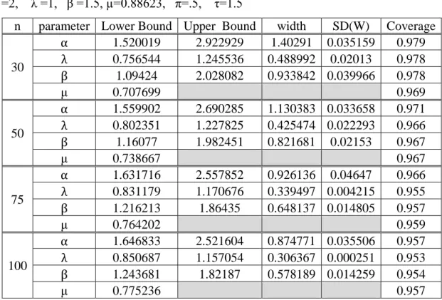
β =1.5, µ=0.9027, π=.5, τ=1 ... 26 Table 2.5 Coverage For Asymptotic 95% C.I.s α =1.5, λ =1, β =1.5, µ=0.9027,
π=.5, τ=1.5 ... 26 Table 2.6 Coverage of Parametric Bootstrap 95% C.I.s α =1.5, λ =1,
β =1.5, µ=0.9027, π=.5, τ=1.5 ... 27 Table 2.7 Coverage of Nonparametric Bootstrap 95% C.I.s α =1.5, λ =1,
β =1.5, µ=0.9027, π=.5, τ=1.5 ... 27 Table 2.8 Coverage of Asymptotic 95% C.I.s α =2, λ =1, β =1.5,
µ=0.88623, π=.5, τ=1 ... 28 Table 2.9 Coverage of Parametric Bootstrap 95% C.I.s α =2, λ =1,
β =1.5, µ=0.88623, π=.5, τ=1 ... 28 Table 2.10 Coverage of Nonparametric Bootstrap 95% C.I.s α =2, λ =1,
β =1.5, µ=0.88623, π=.5, τ=1 ... 29 Table 2.11 Coverage of Asymptotic 95% C.I.s α =2, λ =1, β =1.5, µ=0.88623, π=.5,
τ=1.5 ... 29 Table 2.12 Coverage of Parametric Bootstrap 95% C.I.s α =2, λ =1,
β =1.5, µ=0.88623, π=.5, τ=1.5 ... 30 Table 2.13 Coverage of Nonparametric Bootstrap 95% C.I.s α =2, λ =1,
β =1.5, µ=0.88623, π=.5, τ=1.5 ... 30 Table 2.14 Coverage of Asymptotic 95% C.I.s α =2, λ =1, β =1.5,
µ=0.88623, π=.667, τ=1 ... 31 Table 2.15 Coverage of Parametric Bootstrap 95% C.I.s α =2, λ =1,
β =1.5, µ=0.88623, π=.667, τ=1 ... 31 Table 2.16 Coverage of Nonparametric Bootstrap 95% C.I.s α =2, λ =1,
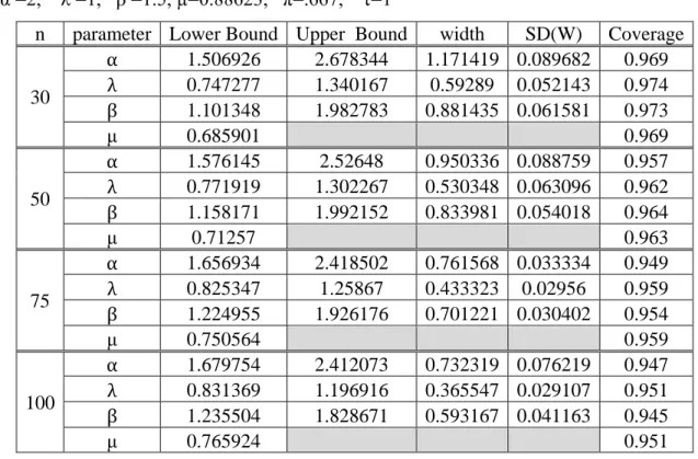
β =1.5, µ=0.88623, π=.667, τ=1 ... 32 Table 2.17 Coverage of Asymptotic 95% C.I.s α =2, λ =1, β =1.5, µ=0.88623,
Table 2.18 Coverage of Parametric Bootstrap 95% C.I.s α =2, λ =1,
β =1.5, µ=0.88623, π=.667, τ=1.5 ... 33
Table 2.19 Coverage of Nonparametric Bootstrap 95% C.I.s α =2, λ =1, β =1.5, µ=0.88623, π=.667, τ=1.5 ... 33
Table 2.20 Coverage of Asymptotic 95% C.I.s α =2, λ =1, β =2, µ=0.88623, π=.5, τ=1 ... 34
Table 2.21 Coverage of Parametric Bootstrap 95% C.I.s α =2, λ =1, β =2, µ=0.88623, π=.5, τ=1 ... 34
Table 2.22 Coverage of Nonparametric Bootstrap 95% C.I.s α =2, λ =1, β =2, µ=0.88623, π=.5, τ=1 ... 35
Table 2.23 Coverage of Asymptotic 95% C.I.s α =2, λ =1, β =2, µ=0.88623, π=.5, τ=1.5 ... 35
Table 2.24 Coverage of Parametric Bootstrap 95% C.I.s α =2, λ =1, β =2, µ=0.88623, π=.5, τ=1.5 ... 36
Table 2.25 Coverage of Nonparametric Bootstrap 95% C.I.s α =2, λ =1, β =2, µ=0.88623, π=.5, τ=1.5 ... 36
Table 2.26 Coverage of Asymptotic 95% C.I.s α =2, λ =1, β =2, µ=0.88623, π=.667, τ=1 ... 37
Table 2.27 Coverage of Parametric Bootstrap 95% C.I.s α =2, λ =1, β =2, µ=0.88623, π=.667, τ=1 ... 37
Table 2.28 Coverage of Nonparametric Bootstrap 95% C.I.s α =2, λ =1, β =2, µ=0.88623, π=.667, τ=1 ... 38
Table 2.29 Coverage of Asymptotic 95% C.I.s α =2, λ =1, β =2, µ=0.88623, π=.667, τ=1.5 ... 38
Table 2.30 Coverage of Parametric Bootstrap 95% C.I.s α =2, λ =1, β =2, µ=0.88623, π=.667, τ=1.5 ... 39
Table 2.31 Coverage of Nonparametric Bootstrap 95% C.I.s α =2, λ =1, β =2, µ=0.88623, π=.667, τ=1.5 ... 39
Table 3.1 Properties of the Hazard Function ... 47
Table 3.2a GE Parameters, Acceleration Factor, and Type I Censoring ... 61
Table 3.2b GE Parameters, Acceleration Factor, and Type I Censoring ... 62
Table 3.3 Coverage of Asymptotic 95% C.I.s α =1.5, λ =1, β =1.5, µ= 1.2804, π=.5, τ=1 ... 63
Table 3.4 Coverage of Parametric Bootstrap 95% C.I.s α =1.5, λ =1, β =1.5, µ= 1.2804, π=.5, τ=1 ... 63
Table 3.5 Coverage of Nonparametric Bootstrap 95% C.I.s α =1.5, λ =1,
β =1.5, µ= 1.2804, π=.5, τ=1 ... 64 Table 3.6 Coverage of Asymptotic 95% C.I.s α =1.5, λ =1, β =1.5,
µ= 1.2804, π=.5, τ=1.5 ... 64 Table 3.7 Coverage of Parametric Bootstrap 95% C.I.s α =1.5, λ =1, β =1.5,
µ= 1.2804, π=.5, τ=1.5 ... 65 Table 3.8 Coverage of Nonparametric Bootstrap 95% C.I.s α =1.5, λ =1, β =1.5,
µ= 1.2804, π=.5, τ=1.5 ... 65 Table 3.9 Coverage of Asymptotic 95% C.I.s α =2, λ =1, β =1.5,
µ=1.5, π=.5, τ=1 ... 66 Table 3.10 Coverage of Parametric Bootstrap 95% C.I.s α =2, λ =1, β =1.5,
µ=1.5, π=.5, τ=1 ... 66 Table 3.11 Coverage of Nonparametric Bootstrap 95% C.I.s α =2, λ =1, β =1.5,
µ=1.5, π=.5, τ=1 ... 67 Table 3.12 Coverage of Asymptotic 95% C.I.s α =2, λ =1, β =1.5, µ=1.5, π=.5,
τ=1.5 ... 67 Table 3.13 Coverage of Parametric Bootstrap 95% C.I.s α =2, λ =1, β =1.5, µ=1.5, π=.5, τ=1.5 ... 68 Table 3.14 Coverage of Nonparametric Bootstrap 95% C.I.s α =2, λ =1, β =1.5,
µ=1.5, π=.5, τ=1.5 ... 68 Table 3.15 Coverage of Asymptotic 95% C.I.s α =2, λ =1, β =1.5, µ=1.5,
π=.667, τ=1 ... 69 Table 3.16 Coverage of Parametric Bootstrap 95% C.I.s α =2, λ =1, β =1.5, µ=1.5, π=.667, τ=1 ... 69 Table 3.17 Coverage of Nonparametric Bootstrap 95% C.I.s α =2, λ =1, β =1.5,
µ=1.5, π=.667, τ=1 ... 70 Table 3.18 Coverage of Asymptotic 95% C.I.s α =2, λ =1, β =1.5, µ=1.5,
π=.667, τ=1.5 ... 70 Table 3.19 Coverage of Parametric Bootstrap 95% C.I.s α =2, λ =1, β =1.5, µ=1.5, π=.667, τ=1.5 ... 71 Table 3.20 Coverage of Nonparametric Bootstrap 95% C.I.s α =2, λ =1, β =1.5,
µ=1.5, π=.667, τ=1.5 ... 71 Table 3.21 Coverage of Asymptotic 95% C.I.s α =2, λ =1, β =2, µ=1.5, π=.5, τ=1
... 72 Table 3.22 Coverage of Parametric Bootstrap 95% C.I.s α =2, λ =1, β =2,
Table 3.23 Coverage of Nonparametric Bootstrap 95% C.I.s α =2, λ =1, β =2, µ=1.5, π=.5, τ=1 ... 73 Table 3.24 Coverage of Asymptotic 95% C.I.s α =2, λ =1, β =2, µ=1.5, π=.5,
τ=1.5 ... 73 Table 3.25 Coverage of Parametric Bootstrap 95% C.I.s α =2, λ =1, β =2, µ=1.5,
π=.5, τ=1.5 ... 74 Table 3.26 Coverage of Nonparametric Bootstrap 95% C.I.s α =2, λ =1,β =2, µ=1.5,
π=.5, τ=1.5 ... 74 Table 3.27 Coverage of Asymptotic 95% C.I.s α =2, λ =1, β =2, µ=1.5, π=.667,
τ=1 ... 75 Table 3.28 Coverage of Parametric Bootstrap 95% C.I.s α =2, λ =1, β =2, µ=1.5,
π=.667, τ=1 ... 75 Table 3.29 Coverage of Nonparametric Bootstrap 95% C.I.s α =2, λ =1 β =2,
µ=1.5, π=.667, τ=1 ... 76 Table 3.30 Coverage of Asymptotic 95% C.I.s α =2, λ =1, β =2, µ=1.5, π=.667,
τ=1.5 ... 76 Table 3.31 Coverage of Parametric Bootstrap 95% C.I.s α =2, λ =1, β =2,
µ=1.5, π=.667, τ=1.5 ... 77 Table 3.32 Coverage of Nonparametric Bootstrap 95% C.I.s α =2, λ =1, β =2,
1. INTRODUCTION
When products are designed to be highly reliable and therefore have a long life-span, standard life testing, where a sample of units is tested under normal use conditions, will not produce a sufficient number of failures to enable the researcher to obtain good estimates of the parameters of interest. One solution to the problem is to subject the specimens in the sample to higher than normal stress levels. The stress factors can be temperature, humidity, pressure, repetitive flexing at a higher than normal rate, or any other variable that can accelerate the failure process. Since the goal of the study is to estimate the parameters of the underlying life distribution and the expected life-span of the products under normal (design) use conditions, a mathematical model that relate the stress level to one or more parameters of the life distribution has to be estimated and then utilized to extrapolate results obtained at high stress levels to those at the normal level. This model that links stress to the distribution parameter(s), however, must be based on well-understood and/or empirically verified relationship (Meeker and Escobar 1998, p. 495). When such a model is available, an accelerated life test (ALT) can be performed where test specimens are subjected to two or more distinct higher than normal stress levels. The higher stress levels accelerate the failure process, thus yielding a sufficient number of un-censored failure data within a reasonable test period. When a reasonable model that links the stress level to distributional parameter(s) is not available, the partially accelerated life test (PALT) procedure is available as an alternative. In PALT, the test specimens are subjected to a single high stress level as well as stress at the normal level.
Each of these accelerated life test methods can be implemented in two different ways, namely using a constant stress protocol or utilizing a step-stress approach to life testing. In the constant stress procedure, independent samples of specimens are assigned to each of the designated high stress levels, and all specimens in a sample are kept at the assigned stress throughout the experiment. That is, the stress is kept constant within a sample. For example, in PALT, some specimens may experience normal stress throughout the experiment while others are subjected to a higher stress level which is kept constant during the test period. In step-stress method, all specimens are first
subjected to one level of stress for a given period of time, and the test specimens that are still functional are subjected to a higher stress level. In this study, the focus will be limited to the constant stress approach so discussions from here on will be on this method only.
In a certain type of constant stress life testing, a sample of product specimens are put to test over a pre-specified test period T and the life spans of the items that failed during this period are recorded. Since not all items on test may fail by time T, the life-span of some specimens are censored. This type of censoring is called Type I censoring. Alternatively, the experimenter can wait until a specific number of items fail and then stop the experiment. For example he/she can wait until 50% of the items fail. In this case we have what is termed as Type II censoring. Since the experimenter sets a specific time at which the experiment will end, the Type I censoring approach is preferable over Type II censoring. The experimenter who conducts a Type II censored experiment will not have a precise idea when the experiment is going to end because the time it takes for a specific percentage of items to fail is a random variable. However, the mathematics of the estimation procedure under Type I censoring can be complicated because the number of failures, R, is a random variable rather than a fixed number as is the case in Type II censoring. The work herein centers on experiments conducted under Type I censoring.
1.1. ACCELERATED LIFE TESTS (CONSTANT STRESS CASE)
In Accelerated Life Tests (ALT), the life-span, X, of a product is assumed to have a distribution (termed the life-distribution) with a probability density function𝑓𝑓�𝑥𝑥,𝜃𝜃�, where 𝜃𝜃 =�𝜃𝜃1,𝜃𝜃2,⋯,𝜃𝜃𝑝𝑝�′is a vector of parameters associated with the distribution such that one or more of the parameters in 𝜃𝜃 are related to the stress S through a relationship whose functional form is known except for a few parameters. For example, θ1 may be related to 𝑆𝑆 through the function: 𝜃𝜃1 =𝑔𝑔(𝑆𝑆,∅0,∅1) =𝑒𝑒𝑥𝑥𝑒𝑒{∅0+∅1𝑆𝑆}. It is assumed that the other parameters in 𝜃𝜃 are not related to S. To estimate the parameters, two independent samples of specimens of the product are tested, with one sample undergoing stress at an accelerated level 𝑆𝑆𝐿𝐿 and the other sample subjected to an even
higher stress level 𝑆𝑆𝐻𝐻. If 𝑆𝑆𝐷𝐷is the stress level at normal (design) use conditions, then we have the ordering𝑆𝑆𝐿𝐿 <𝑆𝑆𝐷𝐷 < 𝑆𝑆𝐻𝐻. From the experimental data, the parameters of the function 𝑔𝑔 are estimated (in the example above we estimate ∅0 and∅1). The parameters
𝜃𝜃𝑖𝑖,𝑖𝑖= 2,3, … .𝑒𝑒 are estimated using combined data from both samples because they do
not depend on the stress level. Then, using the estimated function, g, the value of 𝜃𝜃1 at the design stress level is estimated by the relationship 𝜃𝜃�1 = 𝑔𝑔�𝑆𝑆𝐷𝐷,∅�0,∅�1� This yields an estimate of the life-distribution at normal use stress level.
A Brief Review of Relevant Literature. There are a large number of
1.1.1
publications on ALTs and a relatively smaller but an appreciable number also available for PALTs. For brevity, we will refrain from discussing all of these, but limit the discussion to a select few of these publications. An excellent coverage of Accelerated Life tests is given in Nelson (1990). Other books include Mann, Schafer, and Singapuwalla (1974), Lawless (1982), Viertl (1988), Marvin Rausand and Hsyland (2004) Michelle, Hoang Jr, and David (2006),Guangbin Yang (2007), Tobias and Trindade (2011), and Meeker and Escobar (1998).
One of the more recent publications is Jayawardhana and Samaranayake (2003), that discussed obtaining lower prediction bounds for a future observation from a Weibull population at design (normal use) stress level, using Type II censored accelerated life test data. The scale parameter of the life distribution is assumed to have an inverse power relationship with the stress level. They showed that the method works well when the low and high stresses are reasonably far apart. Alferink and Samaranayake (2011) considered accelerated degradation models and developed confidence intervals for mean life using the Delta method and the bootstrap, assuming lognormal distribution with variance dependent on stress. Another interesting paper is Kamal, et al (2013), who presented a step stress ALT plan that works well. In step stress, the components are first put at a lower stress and the unfailed components are subjected to higher stress after a specific period. More recently, Jayawardhana and Samaranayake (2014), obtained predictive density of a future observation at normal use conditions using ALT method under lognormal life distribution and Type II censoring with non-constant variance.
1.2. PARTIALLY ACCELERATED LIFE TESTS (CONSTANT STRESS CASE)
The main drawback of accelerated life tests is the fact that the functional form of the model that relates stress to the parameters of the life-distribution has to be known. The form of this function can be dependent on the nature of the material the product under study is made of or the construction of the product. For some materials such as electrical insulators, the functional form of g is well known (Nelson, 1990). For some products, especially those constructed of new materials, such a function may not be easily assumed. In many situations, Partially Accelerated Life Tests (PALT) can overcome this problem. In PALT scenario, one set of product specimens are tested at normal use conditions while the other set is tested under high stress conditions. Rather than assume a function that links the model parameter θ1 with stress, it is assumed that at higher stress, θ1 takes a new valueθ1∗ = βθ1. That is, the acceleration changes
θ1through a multiplicative constant. While the mathematics behind estimating both θ1
and θ1∗ as well as the other parameters of the life distribution is not simple, the PALT methodology avoids the assumption of the linkage function g thus eliminating the chance of using an incorrect functional form. The main drawback of the PALT procedure is that one set of product specimens has to be tested at the normal use stress level thus forcing the experimenter to increase the product test time T in order to ensure that a sufficient number of specimens will fail under normal use conditions. This method, however, is ideal for life testing products such as chemicals, whose usable life-span is moderately long but may not run into many years.
Within the PALT, the literature works mention. Saxena and Zarrin (2013) used the Constant Stress Partially Accelerated Life Test (CSPALT) and assumed Type-I censoring under the Extreme Value Type-III distribution. The Extreme Value Type-III distribution has been recommended as appropriate for high reliability components. The authors used the Maximum Likelihood (ML) method to estimate the parameters of CSPALT model and confidence intervals for the model parameters were constructed. Note that the CSPALT plan is used to minimize the Generalized Asymptotic Variance (GAV) of the ML estimators of the model parameters.
Ismail (2013) derived the maximum likelihood estimators (MLEs) of the parameters of the GE distribution and the acceleration factor when the data are Type-II censored under constant-stress PALT model. The likelihood ratio bounds (LRB) method was used to obtain confidence bounds of the model parameters when the sample size is small. It is also shown that the maximum likelihood estimators are consistent and their asymptotic variances decrease as the sample size increases. The numerical results reported in the paper support the theoretical findings and showed that the estimated approximate confidence intervals for the three parameters are smaller when the sample size is larger.
Abdel-Hamid (2009), considered a constant PALT model when the observed failure times come from Burr(c,k) distribution under progressively Type-II right censoring. The MLEs of the parameters were obtained and their performance was studied through their mean squared errors and relative absolute biases. The paper also showed how to constructed approximate and bootstrap CIs for the parameters. The bootstrap CIs give more accurate results than the approximate intervals for small sample sizes, the Student’s-t bootstrap CIs are better than the Percentile bootstrap CIs in the sense of having smaller widths. However, the differences between the lengths of CIs for the two methods decrease with the increase in sample size.
In this study, we develop PALT methodologies for constructing confidence intervals not only for the distribution parameters and the acceleration factor, but also a lower confidence bound for the mean life, under Type I censoring. Three types of confidence intervals and bounds are considered. They are the asymptotic intervals/bounds constructed from the delta-method and those constructed using the parametric bootstrap or the non-parametric bootstrap. The underlying distributions considered are the Weibull and the Generalized Exponential (GE). Methods for obtaining asymptotic or bootstrap-based confidence bounds for the mean life under PALT are not discussed in currently available literature for any type of life distribution, censoring scheme. Also, not available in current literature on PALT are bootstrap-based methods for constructing confidence intervals for distribution parameters of Weibull and
GE distribution and the acceleration factor under Type I censoring. This research aims to fill this gap.
2. BOOTSTRAP-BASED CONFIDENCE INTERVALS IN PARTIALLY ACCELERATED LIFE TESTING UNDER THE WEIBULL
DISTRIBUTION
2.1 INTRODUCTION
Products which under normal use conditions last for a long period pose a problem in determining their mean life using standard life tests because only a very small fraction of them will fail under a testing period of reasonable duration. In such situations, practitioners resort to accelerated life tests (ALT). As Nelson (1980) puts it: “Accelerated life testing of a product or material is used to get information quickly on its life distribution.” In an ALT scenario, test units are run under two or more high stress levels to accelerate the failure process conditions yielding failure-time data sooner than under normal (design, field) use conditions. A model is fitted to the accelerated failure times and then extrapolated to estimate the life distribution under normal conditions. Alternatively, a known acceleration factor that adjusts a parameter of the life distribution to account for the higher stress is utilized for this purpose. This is quicker, cheaper, and more practical than testing at design use conditions. When there exists a mathematical model, which specifies the life-stress relationship, or an acceleration factor is known, the ALT is a very suitable approach to quickly obtain information useful for estimating the life distribution under normal use conditions. However, there are some situations in which neither the acceleration factor is known nor do life-stress models exist, or are very hard to assume. In such cases partially accelerated life tests (PALT) provide a better approach.
Under the PALT method, a portion of the test units are placed under the normal use stress conditions and the remaining units are tested under a suitably selected higher than normal stress level. The life distribution under the higher stress level is assumed to be the same as that under normal use, but with the scale parameter multiplied by an acceleration factor. This factor is estimated together with the other distribution parameters. Since there are more failure data from the units that received higher than
normal stress level, the combined data provide better estimates of the common parameters.
One drawback of the PALT method is that unlike in the ALT, some units have to be tested under normal use. Thus this method is not suitable for components that are very long lasting. But items such as chemicals that have shelf-lives that are measured in months or a year or two can be tested using this method.
In the following, we develop PALT-based methodologies to obtain confidence bounds for the mean life and confidence intervals for the acceleration factor as well as the distribution parameters when the underlying distribution is Weibull. Type I censoring is also assumed. The methodologies considered are asymptotic methods as well as those relying on the parametric or the non-parametric bootstrap. This research extends the work of Ismail (2013) who assumed Type II censoring and employed only the traditional large sample approach to obtaining prediction intervals. While Ismail’s work assumed a Generalized Exponential distribution as the underlying life distribution, we assume the Weibull in this study. The performances of the three methods are compared using a Monte-Carlo simulation study.
2.1.1 A Brief Review of Relevant Literature. Partial accelerated life test (PALT) is the one of methods used for reliability demonstration and prediction of components at normal conditions using data obtained at accelerated condition. It is a type of testing method that enables one to quickly get information over a variety of conditions, and is therefore an important tool for the reliability engineer. A brief outline of previous work on PALT is given below.
Nelson (1990) showed that the stress can be applied in two ways; as constant stress over the test period or in a step-stress fashion. In step-stress partially accelerated life tests (SS-PALT), a test item is first run at normal use conditions and, if it does not fail for a specified time, then it is subjected to a higher than normal stress level for
another testing period. The SS-PALT were studied extensively by many authors, for example: Preeti Wanti Srivastava, Mittal (2010), Abdel-Hamid (2009).
However, the constant-stress PALT runs every item at either normal use condition or accelerated use condition only. Thus, we have two samples and units in each sample are run at a constant stress level unique to that sample, the levels being either normal or a pre-determined higher than normal level. Within the literature on PALTs, the following studies are worth mentioning. Saxena and Zarrin (2013) used the constant stress Partially Accelerated Life Test (CSPALT) and assumed Type-I censoring. The underlying life-distribution they incorporated was the Extreme Value Type-III distribution, which has been recommended as appropriate for high reliability components. The Maximum Likelihood (ML) method was employed by the authors to estimate the parameters of CSPALT model and confidence intervals for the model parameters were also constructed.
Ismail (2013) assumed a constant-stress PALT testing scenario under Type-II censoring. In addition to asymptotic confidence bounds, likelihood ratio bounds (LRB) method employed to obtain confidence bounds of the model parameters in small sample situations. The authors showed that the maximum likelihood estimators are consistent and their asymptotic variances decrease as the sample size increases. They also established that the estimated approximate confidence intervals for the three parameters become narrower with increase in sample size. These asymptotic results were confirmed using numerical simulations.
A constant PALT model was developed by Abdel-Hamid (2009), for the case when the underlying life distribution is Burr(c,k). They considered that sample is subjected to progressive Type-II right censoring. The MLEs of the parameters were obtained and their performance with respect to their mean squared errors and relative absolute biases were investigated. The author also constructed approximate and parameters bootstrap-based confidence intervals (CIs) for the parameters. It was shown that the bootstrap CIs gave more accurate results than the approximate intervals for small sample sizes, and that the Student’s-t bootstrap CIs have smaller widths than the
Percentile bootstrap CIs. The differences between the lengths of CIs for the two methods, however, decreased with on increase in sample size.
2.1.2 The Weibull Distribution. The proposed PALT method is developed for
the case where the underlying life distribution is Weibull. The Weibull probability density function is given by:
(
; ,)
1 , 0, 0, 0, x x f x e x α α λ α α λ α λ λ λ − − = > > > (1)And the cumulative distribution function is:
(
; ,)
1 , x F x e α λ α λ = − − (2)where α is the shape parameter and
λ
the scale parameter.Note that the Weibull distribution is used extensively in reliability literature because of the different shapes its hazard function can take based on different shape parameter values. The hazard (or the failure rate) function of the Weibull distribution is given by:
(
; ,)
( )
( )
1 1 f x x h x F x α α α λ λ λ − = = − . (3)2.2 THE PROPOSED PALT METHOD AND BOOTSTRAP INTERVALS
The following assumptions are made regarding the proposed PALT method.
1. The total number of units under test is n.
2. π denotes the proportion of sample units allocated to accelerated condition
3.n
(
1−π)
=nπ units, where π = −1 π, are allocated to normal (field) use conditions. 4. nπunits are allocated to the high stress condition (subject to acceleration)Likelihood Function under Type I Censoring and Asymptotic C.I.s. 2.2.1
Under Type I censoring, the censoring time, τ is fixed but the number of failures observed during the test duration τ is a random variable, say R.
i
x
: Observed lifetime of item i tested at the normal (field) use conditions.
j
y
: Observed lifetime of item j tested at high stress conditions.
i
u
δ
: Indicator function denoting the censoring state of ith observation under normal use condition, with δ =ui 1if the observation is uncensored.
j
a
δ
: Indicator function denoting the censoring state of jth observation under high stress condition, withδaj =1 if the observation is uncensored.
u
n : Number of items that failed at normal use condition.
a
n :Number of items that failed at high stress condition. τ: The censoring time of the life test (for all units).
( )1 ( )nu
x ≤≤ x ≤τ : Ordered failure times at normal use condition.
( )1 ( )nu
y ≤≤ y ≤τ : Ordered failure times at high stress condition.
β: Denotes the acceleration factor
(
β >1)
.In type I censoring, τ is fixed but the number of failure values observed in time τ is a random variable. The number of items, R, failing before time τ is assumed to follow a binomial distributionRBin n p
(
,)
, wherep F(
; ,)
1 eX α τ λ τ α λ − = = − , under normal
use conditions. Under high stress conditions the number of items failing will have a
BinomialBin n p
(
, *)
, distribution where *(
; , ,)
1 .x p F e X α β λ τ α λ β − = = − Then, for
observation i under normal use conditions, we have, 1 , 1, 2, , . 0 0 / i i u x i n w τ δ = ≤ = π (4)
Similarly, for observation j under a high stress condition, we have,
1 , 1, 2, , , 0 0 / j j a y j n w τ δ = ≤ = π (5) 1 i, 1 j, i u j a u a δ = −δ δ = −δ with
1 ( ) ( , ), i i n u u i Ber p Bin n p π δ δ π = ⇒
∑
(6) 1 ( ) ( , ). j j n a a j Ber p Bin n p π δ δ π = ⇒∑
(7) We also have, under normal use conditions,(
) (
)
( ) 1 ; , ( ) 1 1 , 1 1, , x x P X x e F x P X x X P X e e x e x α α α α λ τ τ λ λ τ λ α λ τ τ τ τ τ − − − − ≤ − = ≤ ≤ = = ≤ − − ≤ = − > (8) and(
)
(
(
)
)
1 ; , ; , . ; , 1 x X x X x e f x f x F e α α α λ τ λ α α λ λ λ α λ τ τ α λ − − − = = − (9)Thus, givenR=nu, the conditional density of the first r failure times under a normal use condition is equivalent to the joint density of an ordered random sample of sizenu
from a truncated Weibull distribution, given by
(
)
(
)
1 1 (1) ( ) ( ) 1 1 1 1 , , ! ; , ! 1 ! . 1 i u u u nu i u i u u x i n n n u u i u i i x n n i u n i x e f x x R n n f x n e e x n e α α α α α λ τ τ λ λ λ α τ λ α λ λ α λ α λ λ = − − − = = − − = − = = = − ∑ = − ∏
∏
∏
(10)The joint density of obtainingR=nuordered observations at the values ( )1 , , ( )
u
n
x x
(
(1), , (nu)) (
(1), , (nu) u)
( ;u , ) f x x = f x x R=n bin n nπ p =(
)
1 1 1 ! 1 1 nu i u i u u u u x n n n n n i u n i u e n x n p p n e α α λ α π τ λ α π λ λ = − − − = − ∑ = − − ∏
( )
(
)
( )
(
)
1 1 1 1 1 ! 1 ! 1 ! ! nu i u i u u u u nu u i u i x n n n n n i n i u n n x n i u e n x e e n n e n x e e n n α α α α α α λ π α τ τ λ λ τ λ π α τ λ λ α π λ π λ π α π λ λ = = − − − − − = − − − − − ∑ = − − − ∑ = − ∏
1 . u n i=∏
Therefore, we have(
)
1 1 (1) ( ) 1 , , . nu u i u u i u n n x n n i n i x f x x e e α α π α τ λ λ α λ = λ − − − − = ∑ ∝ ∏
In a fashion similar to the argument made about the joint density of observations under normal use conditions, givenR=na the conditional density of the first r failure times
under acceleration is equivalent to the joint density of an ordered random sample of size
a
n from a truncated accelerated Weibull distribution. Therefore, for an item tested at accelerated condition, the probability density function is given by
(
; , ,)
1 , 0, 0, 0, 1, x x f x e x α β α λ βα β α λ β α λ β λ λ − − = > > > > whereY =β−1X.(
)
(
)
1 1 (1) ( ) ( ) 1 1 1 1 , , ! ; , , ! 1 ! . 1 j a a a na j a i a a y j n n n a a i a j j y n n j a n j y e f y y R n n f y n e e y n e α α α α β α λ τ βτ λ β λ α βτ λ β αβ λ λ α λ β βα β λ λ = − − − = = − − = − = = = − ∑ = − ∏
∏
∏
(11)The joint density of obtainingR=naordered observations at the values (1), , ( )
a
n
Y Y
before time, may be expressed as
(
) (
)
* (1), , (na) (1), , (na) a ( ;a , ) f y y = f y y R=n bin n nπ p( ) (
)
( )
(
)
1 1 1 * * 1 1 ! 1 1 ! 1 ! 1 na j a i a a a a na j a i a y n n n n n j a n j a y n j n a e y n n p p n e e y n e n n e α α α α α β λ α π βτ λ β λ α βτ λ βτ λ βα β π λ λ βα β π λ π λ = = − − − = − − − − − ∑ = − − ∑ = − − − ∏
( )
(
)
1 1 1 1 ! , ! a a a na a j a a i n n n n j n n y n n j j a e y n e e n n α α α π βτ λ π β α βτ λ λ β π βα π λ = λ − − = − − − − = ∑ = − ∏
∏
thus,(
)
1 1 (1) ( ) 1 , , , na a j a a i a n n y n n j n j y f y y e e α α π β α βτ λ λ β βα λ = λ − − − − = ∑ ∝ ∏
and the total likelihood function for
(
)
1 1
1; u, , n ; un , 1; a , , n ; an
x δ xπ δ π y δ yπ δ π can be expressed as follows:
(
)
(
)
(
)
1 1 1 1 1 , , , , , , , , i i j j u j ui ui j uj i i u i u u j u y x n n j i i j x i L L x y L x L y y x e e e e x e α α δ α δ α β δ α δ α τ βτ π π λ λ λ λ α λ α λ β α λ δ α λ β δ β α βα λ λ λ λ α λ λ − − − − − − = = − − = = = = ∏
∏
1 1 1 1 1 . j u a u a y n n n n j i i n j j n y e e e α α τ α α β βτ α π π λ λ βα β λ λ λ − − − − = = + = = + ∏
∏
∏
∏
(12)The MLE’s of the parameters can estimated numerically by minimizing the log likelihood function.
(
)
(
)
(
)
1 1 1 1 1 1 1 1 1 1 1 ln ln , , , ln ln 1 ln ln ln ln 1 ln . u u u u u a a a a a a n n n n n i i i i i i i n n n n n n n j j j j j j j j n L L x y l x x l y y α π α α π α α λ β τ α λ α λ λ λ β β βτ α λ β α λ λ λ = = = = = + = = = = = = + ⇒ = = ⇒ = − + − − − + − + + − − − ∑
∑
∑
∑
∑
∑
∑
∑
∑
∑
∑
(13)(
)(
)
7 8 1 1 1 1 ln ln ln u a u a n n n n u a a i j i j i n j n l n n n α α π τ π βτ α λ β ψ ψ λ λ = = = + = + ⇒ = + − + + + − − ∑
∑
∑
∑
(
)(
)
(
)
(
)
7 8 1 1 ln ln ln . u a n n u a a i j i j u a l n n n n n n n α α α λ β ψ ψ τ βτ π π λ λ = = ⇒ = + − + + + − − − − ∑
∑
The score equations are obtained by differentiating the log likelihood with respect to the parameters and setting them to zero. These equations are:
(
)
(
)
1 2 1 1 3 5 ln ln 0, u a n n j u a i i j i j u a y n n x l n n n n β ψ ψ α α λ λ π ψ π ψ = = + ∂ ⇒∂ = + − + − − − − − =∑
∑
(14)(
)
(
)
1 1 1 0, u a n n j i u a i j y x l n n n n α α α α β α π τ π βτ λ λ λ λ = λ = λ ∂ ⇒ = + − + − + + = ∂ ∑
∑
(15) and(
)
1 1 0. a n j a j y l n n α α β α π βτ β λ λ = λ ∂ ⇒ = − − − = ∂ ∑
(16)Now, we have a system of three nonlinear equations in three unknownsα λ, ,andβ. It is clear that a closed form solution is very difficult to obtain. Therefore, an
iterative procedure must be used to find a numerical solution of the above system.
Asymptotic confidence intervals for parameter θ =
(
α λ β, ,)
can be obtained using the following convergence in distribution result;Result 2.1
The MLEs obtained from the above procedure has the asymptotic distribution given by the following convergence result:
(
ˆ)
(
ˆ) (
ˆ)
1(
)
, ,0
, , , , n α α λ λ β β I− α λ β − − − − → where theI =
(
α λ β, ,)
is the fisher information matrix given by(
)
( )
( )
( )
( )
( )
( )
( )
( )
( )
2 2 2 2 11 12 13 2 2 2 21 22 23 2 31 32 33 2 2 2 2 , , . l l l I I I l l l I I I I I I I l l l α λ α β α α αλ αβ α λ β λα λ λβ λ α λ λ β βα βλ β β α β λ β ∂ ∂ ∂ ∂ ∂ ∂ ∂ ∂ ∂ ∂ ∂ = = ∂ ∂ ∂ ∂ ∂ ∂ ∂ ∂ ∂ ∂ ∂ ∂ ∂ Proof: A proof that shows that the regularity conditions needed for asymptotic normality for Weibull parameters estimates under Type I censoring in the PALT setup is given in the appendix. Note that since the Weibull distribution belongs to the log-location-scale family and the distributions in this family satisfy the regularity conditions needed, the above asymptotic result does hold for MLE estimators of the Weibull parameters (see Escobar and Meeker (2000)), but their results do not consider the case where PALT data are used. Thus, the proof given in the appendix is of importance.
The elements of the 3x3 matrix I I, ij
( )
θ , i j, =1, 2, 3, can be approximated by( ) (
ˆ ˆ, ,ˆ ˆ)
ij ij I θ = I α λ β ,( )
2( )
ˆ ˆ . ij i j l I θ θ θ θ θ θ = ∂ = ∂ ∂(
)
(
)
2 3 5 1 2 2 2 1 1 2 2 , u a n n u a u a i j i j n n l nπ n ψ nπ n ψ ψ ψ α α = = + ∂ = + − + − + + ∂∑
∑
(17)(
) (
)
(
)
2 2 2 u a 1 u a , l n n n n n n α α α α π τ π βτ λ λ λ λ ∂ = + − − − + − ∂ (18)(
)(
)
(
)
2 2 2 1 1 1 1 , a n j a j y l n n α α β α α π βτ α λ λ β β = ∂ = − + − − + − ∂ ∑
(19)(
)
(
)
2 7 8 ln , a i j u a l n n n n n α α τ βτ β ψ ψ π π α β λ λ ∂ = + + − − − − ∂ ∂ (20)(
)
(
)
2 4 6 4 6 1 1 1 , u a n n u a u u i j i j l n n nπ n ψ nπ n ψ ψ ψ α λ λ = = ∂ − = + − − − − − − ∂ ∂ ∑
∑
(21) and(
)
2 2 1 , a n j a j y l n n α α β α π βτ β λ λβ λ = λ ∂ = − + ∂ ∂ ∑
(22) where 1 2 3 4 4 5 ln , ln , ln , ln 1 , ln 1 , ln , j j i i i j i i i y y x x x x α α α α α α β β ψ ψ λ λ λ λ τ τ τ τ ψ ψ α λ λ λ λ βτ βτ ψ α ψ λ λ λ λ = = = = + = + = (
)
(
)
6 6 7 8 ln 1 , ln 1 , 1 ln , 1 ln . j j j j j i i i j y y y y x x α α α α β β βτ βτ ψ α ψ α λ λ λ λ β β ψ α ψ α λ λ λ λ = + = + = − − = − − Now by employing the standard z-based confidence interval formulations,
( )
( )
( )
1 1 1 2 11 ˆ 2 22 ˆ ˆ 2 33 ˆ ˆ Zγ I ˆ , Zγ I , Zγ I α ± − α λ± − λ β ± − β ,we obtain the confidence intervals for the parameters based on the asymptotic distribution.
The asymptotic confidence interval for the mean life at normal use conditions is given by
( )
2 ˆ Zγ Var ˆ , µ± µwhere Var
( )
µˆ is obtained using the Delta method.2.3 THE BOOTSTRAP RESAMPLING METHODS AND THE
MONTE-CARLO PROCEDURE
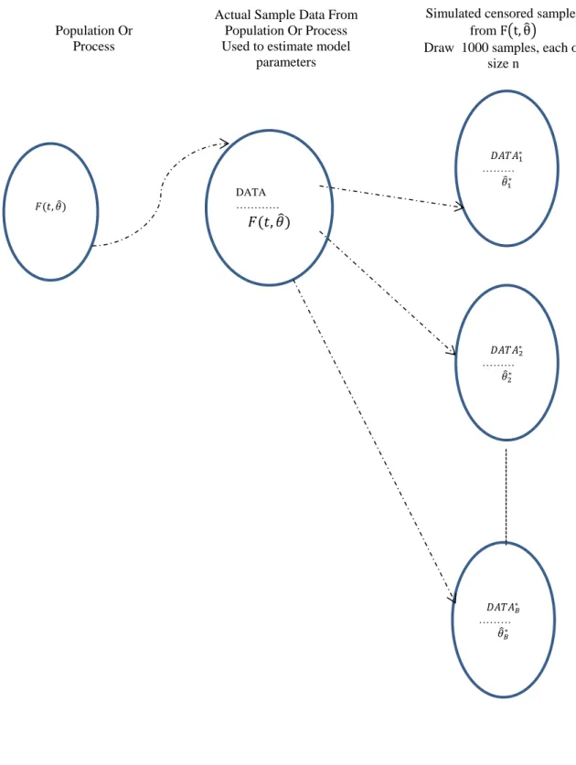
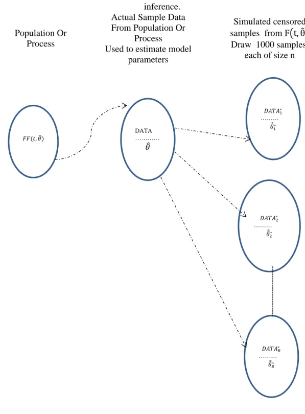
There are two different methods for generating bootstrap sample data. One is the parametric bootstrap, where once the parameters of the underlying distribution are estimated, they are plugged into the assumed distribution and pseudo random numbers then drawn from this estimated distribution to produce the bootstrap sample. The non-parametric bootstrap does not assume a set underlying distribution, but resample from the sample data to produce new samples. The resampling procedure, of course, should be adopted to fit the underlying structure of the problem. For example, in a regression setting, resampling must be done on the residuals of a fitted model rather than from the original data.
In the following, we combine the bootstrap steps with the steps needed to carry out a Monte-Carlo comparison of the proposed methods of building confidence bounds and intervals. The steps for the parametric bootstrap and the non-parametric bootstrap are given separately. Note that the confidence bounds and intervals based on the asymptotic distribution can be computed at each Monte-Carlo simulation sample and does no require bootstrap resampling.
2.3.1 The Proposed Parametric Bootstrap Method and the Monte-Carlo Procedure for Studying its Performance.The Monte-Carlo procedure employed to study the performance of the parametric bootstrap method is described below. The steps
for the parametric bootstrap method for obtaining confidence bounds for α λ, , and β and lower bounds for the mean life are embedded in this procedure and are given in italics. Note that distributional parameters are varied in the study as follows:
(α =1.5,nad2,λ=1,β =1.5,and2) with𝜇𝜇= 𝜆𝜆Γ �1 + 1
𝛼𝛼�. The censoring time was set at 𝜏𝜏=1, and1.5. Note that without loss of generality, scale parameter λcan be set at 1.
(1) For fixed values of n and 𝜋𝜋, generate a random sample 𝑥𝑥𝑖𝑖,𝑖𝑖= 1,2, … ,𝑛𝑛𝜋𝜋 from the Weibull (𝛼𝛼,𝜆𝜆) distribution. This would be considered data from the normal use sample. Similarly, generate the data set𝑦𝑦𝑗𝑗,𝑗𝑗 = 1,2, … ,𝑛𝑛𝜋𝜋, representing the sample under the high stress condition, from the Weibull (𝛼𝛼,𝛽𝛽𝜆𝜆) distribution. (2) Use the ML method to estimate the parameters with the same censoring time τ
used for both samples. In this study, the nonlinear equations of the maximum likelihood estimates were solved iteratively using the Newton Raphson method.
(3) Employ the resulting estimates of the parameters and acceleration factor to construct asymptotic confidence limits with confidence level at 𝛾𝛾 = 0.95. Also, plug-in the MLEs into the Fisher Information matrix to obtain the asymptotic variance and covariance matrix of the estimators and then use them in the delta method to compute the lower bound for mean life.
(4) Replace the unknown parameters,𝛼𝛼,𝜆𝜆, in the Weibull distribution for the normal use case with their MLEs, 𝛼𝛼�,𝜆𝜆̂, and utilize the estimated distribution to generate a bootstrap sample 𝑥𝑥𝑖𝑖∗ ,𝑖𝑖 = 1,2, … ,𝑛𝑛𝜋𝜋 of size 𝑛𝑛𝜋𝜋.Censor the data based on the censoring time τ.
(5) Similarly replace the unknown parameters,𝛼𝛼,𝜆𝜆,𝛽𝛽 in the Weibull distribution for the high stress case with their MLEs, 𝛼𝛼�,𝜆𝜆̂,𝛽𝛽̂ and utilize the estimated distribution to generate a bootstrap sample 𝑦𝑦𝑗𝑗∗ ,𝑗𝑗= 1,2, … ,𝑛𝑛𝜋𝜋 of size 𝑛𝑛𝜋𝜋. Censor the data based on the censoring time τ.
(6) Re-estimate the Weibull parameters of the normal use distribution were using the combined bootstrap samples. Denote the bootstrap sample-based MLEs of
𝛼𝛼,𝜆𝜆,𝛽𝛽𝑎𝑎𝑛𝑛𝑎𝑎𝜇𝜇 obtained at bootstrap step k by 𝛼𝛼�∗(𝑘𝑘),𝜆𝜆̂∗(𝑘𝑘),𝛽𝛽̂∗(𝑘𝑘)𝑎𝑎𝑛𝑛𝑎𝑎𝜇𝜇̂∗(𝑘𝑘) respectively.
(7) Repeat Steps (4) to (6) 1,000 times. Construct the empirical distributions of the bootstrap estimates 𝛼𝛼�∗(𝑘𝑘),𝜆𝜆̂∗(𝑘𝑘),𝛽𝛽̂∗(𝑘𝑘)𝑎𝑎𝑛𝑛𝑎𝑎𝜇𝜇̂∗(𝑘𝑘), k=1, 2, …, 1,000
(8) Use the empirical distributionsobtained from bootstrap estimates to construct, confidence interval for 𝛼𝛼,𝜆𝜆,𝛽𝛽using quantiles at �1−𝛾𝛾
2 �100% and 1− � 1−𝛾𝛾
2 �100% of the
respective empirical distribution as the lower and upper bounds respectively. Use the (1− 𝛾𝛾)100% quantile of the empirical distribution of 𝜇𝜇̂∗(𝑘𝑘) , k=1, 2, …, 1,000, as the lower bound for𝜇𝜇.
(9) Repeat steps (1) through (8) 1,000 times and compute the average number of times each parameter fell within the bound(s). This would yield an estimate of the
expected coverage for each interval. For each parameter except𝜇𝜇, the widths of the two sided interval computed in Steps (3) and (8) are averaged to obtained an estimate of the expected, width.
2.3.2 The Proposed Nonparametric Bootstrap Method and the
Monte-Carlo Procedure for Studying its Performance.The Monte-Monte-Carlo procedure employed to study the performance of the nonparametric bootstrap method is described below. The steps for the parametric bootstrap method for obtaining confidence bounds for
𝜶𝜶,𝝀𝝀,𝒂𝒂𝒂𝒂𝒂𝒂𝜷𝜷 and lower binds for the mean life are imbedded in this procedure and given in italics.
(1) For fixed values of n and 𝜋𝜋, generate a random sample 𝑥𝑥𝑖𝑖,𝑖𝑖 = 1,2, … ,𝑛𝑛𝜋𝜋 from the Weibull (𝛼𝛼,𝜆𝜆) distribution. This would be considered data from the normal use sample. Similarly, generate the data set𝑦𝑦𝑗𝑗,𝑗𝑗= 1,2, … ,𝑛𝑛𝜋𝜋, representing the sample under the high stress condition, from the Weibull (𝛼𝛼,𝛽𝛽𝜆𝜆) distribution.
(2) Obtain a bootstrap resample from each of the two samples generated in Step (1) above, with each bootstrap sample of size πn (or πn) obtained by sampling with replacement from the respective sample obtained in (1).
(3) New “bootstrap estimates” 𝛼𝛼�∗,𝜆𝜆̂∗,𝑎𝑎𝑛𝑛𝑎𝑎𝛽𝛽̂∗ are computed from the combined bootstrap sample using the ML method as described in Step (2) given in Section 2.3.1. Also estimate the mean life µ under normal conditions, accounting for the censoring.
(4) Repeat the process given in Steps (2) and (3) 1,000 times and obtain the empirical distributions of 𝛼𝛼�∗,𝜆𝜆̂∗, 𝑎𝑎𝑛𝑛𝑎𝑎�𝛽𝛽∗..
(5) Using the empirical distributions of the 𝛼𝛼�∗,𝜆𝜆̂∗, 𝑎𝑎𝑛𝑛𝑎𝑎 𝛽𝛽̂∗ obtained from bootstrap estimates, construct confidence interval for 𝛼𝛼,𝜆𝜆,𝑎𝑎𝑛𝑛𝑎𝑎𝛽𝛽using respective quantiles at �1−𝛾𝛾
2 �100% and 1− � 1−𝛾𝛾
2 �100%.
(6) Using the empirical distributions of the mean 𝜇𝜇̂∗ obtained from bootstrap estimates, construct the lower confidence bound for 𝜇𝜇 is using quantile at
(1− 𝛾𝛾)100% .
(7) Coverage probabilities were computed based on 1,000 simulation runs by repeating Steps (1) – (6).
Population Or Process
Actual Sample Data From Population Or Process Used to estimate model
parameters
Simulated censored samples from F�t,�
Draw 1000 samples, each of size n
Figure 2.1.Illustrates the parametric bootstrap resampling method
𝐹𝐹(𝑡𝑡,𝜃𝜃�) 𝐷𝐷𝐷𝐷𝐷𝐷𝐷𝐷1∗ 𝜃𝜃�1∗ ……… 𝐷𝐷𝐷𝐷𝐷𝐷𝐷𝐷2∗ 𝜃𝜃�2∗ ……… 𝐷𝐷𝐷𝐷𝐷𝐷𝐷𝐷𝐵𝐵∗ 𝜃𝜃�𝐵𝐵∗ ……… 𝐹𝐹(𝑡𝑡,𝜃𝜃�) DATA …………
inference.
Population Or Process
Actual Sample Data From Population Or
Process
Used to estimate model parameters
Simulated censored samples from F�t,�
Draw 1000 samples, each of size n
Figure 2.2. Illustrates the nonparametric bootstrap resampling for parametric inference. 𝐹𝐹𝐹𝐹(𝑡𝑡,𝜃𝜃�) 𝐷𝐷𝐷𝐷𝐷𝐷𝐷𝐷1∗ 𝜃𝜃��1∗ ……… 𝐷𝐷𝐷𝐷𝐷𝐷𝐷𝐷2∗ 𝜃𝜃��2∗ ……… 𝐷𝐷𝐷𝐷𝐷𝐷𝐷𝐷∗𝐵𝐵 𝜃𝜃��𝐵𝐵∗ ……… 𝜃𝜃� DATA …………
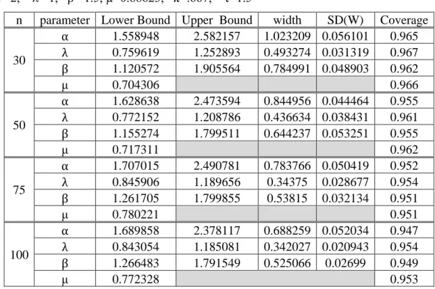
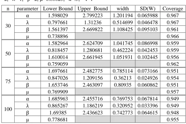
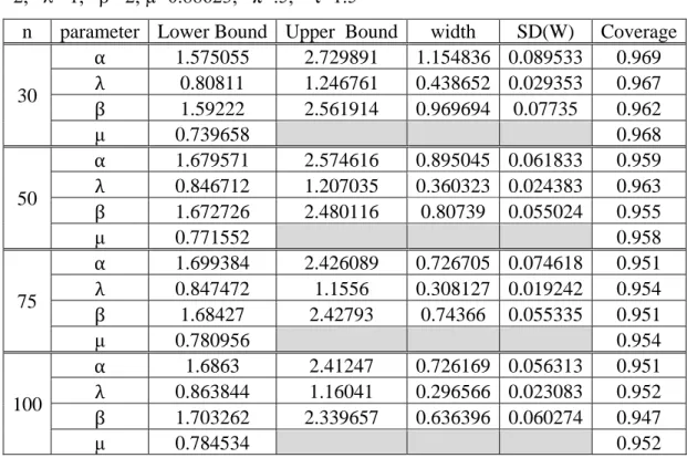
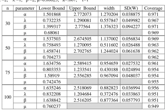
2.4 MONTE-CARLO SIMULATION RESULTS AND DISCUSSION
All simulations results reported here are for α = (1.5, and 2) and λ = 1, with the acceleration factor 𝛽𝛽 set at 1.5 and 2.0. The censoring parameter 𝜏𝜏 was set at values 1, and 1.5
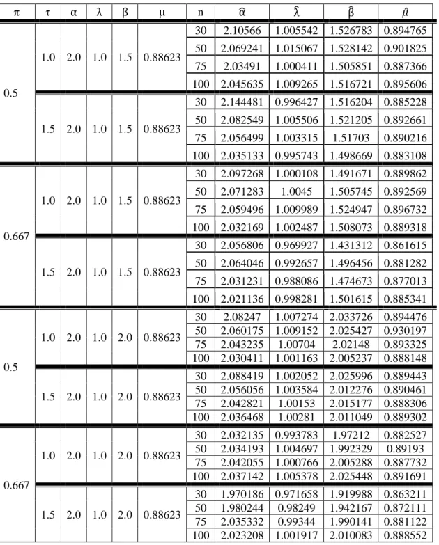
The simulation study was conducted using a computer code written in Matlab, and the simulation results are reported in Table 2.1a to Table 2.31. Tables 2.1a and 2.1b show the results of the maximum likelihood estimation of
(
α λ β, , ,andµ)
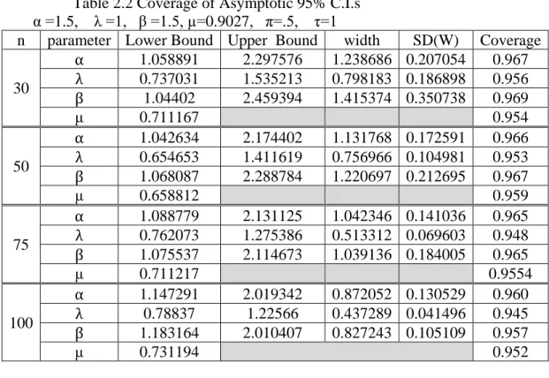
. The estimated expected values of the MLEs are reasonably close to the true values, even for n=30. There is no discernible pattern linking the means of the estimates to changes in the parameter values, at least over the range of parameter values considered in this study. Tables 2.2 to 2.31 show the performance of the asymptotic, parametric bootstrap, and nonparametric bootstrap confidence intervals for(
α λ, , andβ)
at the 95% confidence level and the performance of the Asymptotic, Parametric Bootstrap, and Nonparametric Bootstrap based 95% confidence bound of mean-life under normal conditions.Table 2.1a Weibull Parameters, Acceleration Factor, and Type I Censoring
π τ α λ β μ n α� λ� β� 𝜇𝜇̂ 0.5 1.0 1.5 1.0 1.5 0.9027 30 1.576672 1.043488 1.54321 0.949033 50 1.553463 1.014072 1.565054 0.920318 75 1.543858 0.983789 1.485776 0.891226 100 1.537005 1.015341 1.539113 0.918978 1.5 1.5 1.0 1.5 0.9027 30 1.615358 0.981995 1.516009 0.886497 50 1.564676 0.986138 1.499799 0.890782 75 1.538481 1.016195 1.531349 0.919195 100 1.518111 1.008931 1.522719 0.911857