Efficient Deep Reinforcement Learning via Planning, Generalization, and Improved Exploration

(1)

Efficient Deep Reinforcement Learning via

Planning, Generalization, and Improved

Exploration

by

Junhyuk Oh

A dissertation submitted in partial fulfillment

of the requirements for the degree of

Doctor of Philosophy

(Computer Science and Engineering)

in the University of Michigan

2018

Doctoral Committee:

Professor Satinder Singh Baveja, Co-Chair

Associate Professor Honglak Lee, Co-Chair

Assistant Professor Jia Deng

(2)

Junhyuk Oh

[email protected] ORCID iD: 0000-0003-4383-6396

(3)

ACKNOWLEDGEMENTS

First of all, I would like to thank my co-advisors Honglak Lee and Satinder Singh. It has been a great honor to have both of them as my mentors. All of the work presented in this thesis would have not been possible without their advice and valuable insights. They have been not only excellent advisors in research but also very supportive of my academic career. Working with Honglak and Satinder as a PhD student was one of the best decisions that I have ever made.

I would also like to thank Richard Lewis and Jia Deng for serving on my thesis committee and providing constructive feedback on the thesis. It was also a great pleasure to collaborate with Richard Lewis for my early work.

I am thankful for my former and current lab colleagues: Kihyuk Sohn, Scott Reed, Ruben Villigas, Xinchen Yan, Ye Liu, Yuting Zhang, Seunghoon Hong, Lajanugen Logeswaran, Kibok Lee, Sungryull Sohn, Jongwook Choi, Yijie Guo, Xiaoxiao Guo, Nan Jiang, Zeyu Zheng, Vivek Veeriah, John Holler, Qi Zhang, Shun Zhang, Janarthanan Rajendran, Ethan Brooks, Christopher Grimm, Max Smith, Aditya Modi, and Valliappa Chockalingam. It has been a wonderful experience to share joys and hardships with you.

I am thankful to David Silver for hosting me as an intern at DeepMind where I learned lots of insights from David and truly enjoyed discussions and conversations with Arthur Guez, Hado van Hasselt, Tom Schaul, André Barreto, Joseph Modayil, Thomas Degris, Matteo Hessel, Dan Horgan, Simon Osindero, Sasha Vezhnevets, Vlad Mnih, Nando de Freitas, Daan Wierstra, and Razvan Pascanu. I would like to thank Pushmeet Kohli for hosting me as an intern at Microsoft Research and making a lot of connections to other researchers. I would like to thank Pieter Abbeel, Marc Bellemare, Hugo Larochelle, and John Schulman for giving me an opportunity to present my work at their institutions; Doina Precup, Abdel-Rahman Mohamed, Kyunghyun Cho, Shane Gu, and Junyoung Chung for their advice on my academic career; Youngjae Kim and Jaeho Im for being long-term friends in Ann Arbor.

Finally, this thesis is dedicated to my parents and my wife for their love and support. Especially, I would like to thank my wife, Sona Jeong, for being always very supportive and bringing happiness to my life.

(4)

LIST OF FIGURES

Figure

3.1 Proposed encoding-transformation-decoding network architectures. . . 19

3.2 Example of predictions over 250 steps in Freeway. . . 24

3.3 Mean squared error over 100-step predictions . . . 25

3.4 Comparison between two encoding models . . . 26

3.5 Game play performance using the predictive model as an emulator . . . . 27

3.6 Comparison between two exploration methods on Ms Pacman . . . 29

3.7 Cosine similarity between every pair of action factors . . . 29

3.8 Distinguishing controlled and uncontrolled objects . . . 30

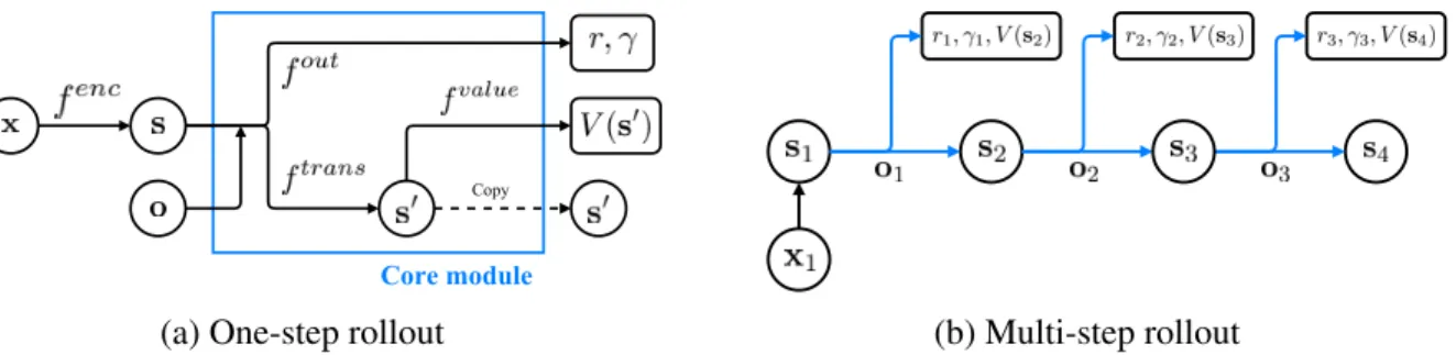
4.1 Value prediction network . . . 36

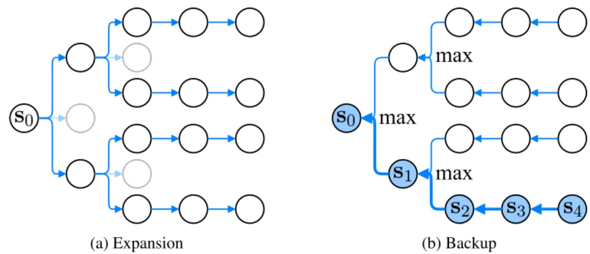
4.2 Planning with VPN . . . 38

4.3 Illustration of learning process. . . 39

4.4 Collect domain . . . 42

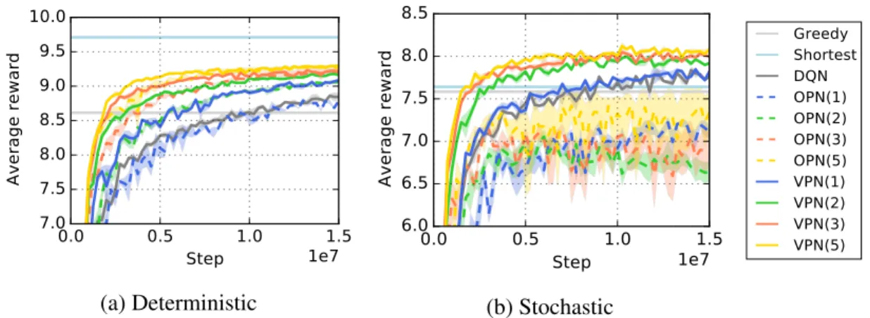
4.5 Learning curves on Collect domain . . . 43

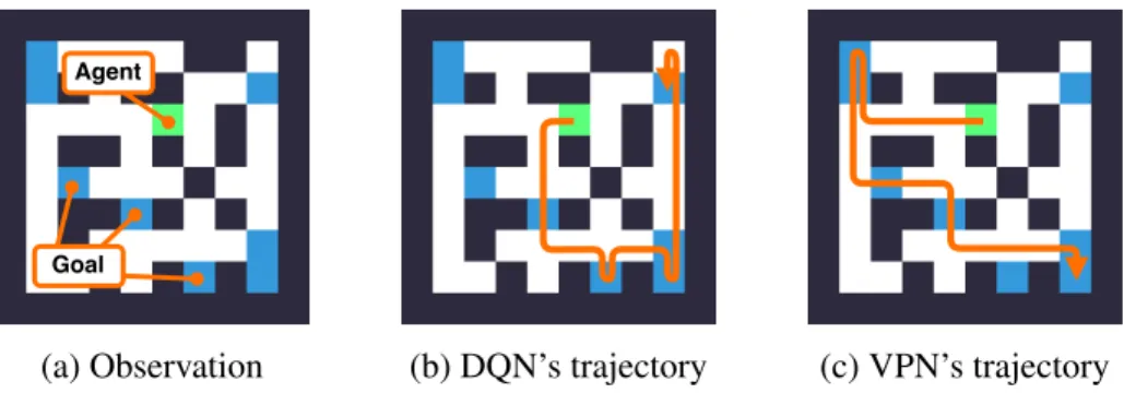
4.6 Example of VPN’s plan . . . 43

4.7 Effect of evaluation planning depth . . . 45

4.8 Learning curves on Atari games . . . 47

4.9 Examples of VPN’s value estimates . . . 47

5.1 Example task in Minecraft . . . 49

5.2 Illustration of memory operations. . . 52

5.3 Illustration of different architectures . . . 52

5.4 Unrolled illustration of FRMQN. . . 54

5.5 Examples of maps . . . 56

5.6 Learning curves for different tasks . . . 58

5.7 Visualization of FRMQN’s memory retrieval . . . 62

5.8 Precision vs. distance . . . 64

6.1 Example of 3D world and instructions . . . 68

6.2 Architecture of parameterized skill . . . 71

6.3 Overview of our hierarchical architecture. . . 76

6.4 Neural network architecture of meta controller. . . 77

6.5 Unrolled illustration of the meta controller . . . 79

6.6 Performance per number of instructions . . . 82

6.7 Analysis of the learned policy . . . 82

(8)

7.2 Key-Door-Treasure domain . . . 95 7.3 Learning curves on hard exploration Atari games . . . 95 7.4 Relative performance of A2C+SIL over A2C across 49 Atari games. . . . 98 7.5 Performance on OpenAI Gym MuJoCo tasks . . . 100 7.6 Performance on delayed-reward versions of OpenAI Gym MuJoCo tasks . 101

(9)

LIST OF TABLES

Table

3.1 Average game score of DQN over 100 plays with standard error . . . 28

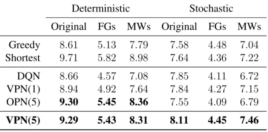
4.1 Generalization performance . . . 44

4.2 Performance on Atari games . . . 46

5.1 Performance on I-Maze . . . 57

5.2 Performance on pattern matching . . . 60

5.3 Performance on random maze . . . 63

6.1 Performance on parameterized tasks . . . 74

6.2 Performance on instruction execution . . . 81

7.1 Comparison to count-based exploration actor-critic agents on hard explo-ration Atari games . . . 97

7.2 Performance of agents on 49 Atari games after 50M steps (200M frames) of training . . . 99

(10)

LIST OF ALGORITHMS

Algorithms

1 Deep Q-Learning . . . 12

2 Synchronous Advantage Actor-Critic (A2C) . . . 15

3 Asynchronous Advantage Actor-Critic (A3C) . . . 15

4 Q-value fromd-step planning . . . 38

5 Subtask update (Soft) . . . 80

(11)

ABSTRACT

Reinforcement learning (RL) is a general-purpose machine learning framework, which considers an agent that makes sequential decisions in an environment to maximize its reward. Deep reinforcement learning (DRL) approaches use deep neural networks as non-linear function approximators that parameterize policies or value functions directly from raw observations in RL. Although DRL approaches have been shown to be successful on many challenging RL benchmarks, much of the prior work has mainly focused on learning a single task in a model-free setting, which is often sample-inefficient. On the other hand, humans have abilities to acquire knowledge by learning a model of the world in an unsupervised fashion, use such knowledge to plan ahead for decision making, transfer knowledge between many tasks, and generalize to previously unseen circumstances from the pre-learned knowledge. Developing such abilities are some of the fundamental challenges for building RL agents that can learn as efficiently as humans.

As a step towards developing the aforementioned capabilities in RL, this thesis develops new DRL techniques to address three important challenges in RL: 1) planning via prediction, 2) rapidly generalizing to new environments and tasks, and 3) efficient exploration in complex environments.

The first part of the thesis discusses how to learn a dynamics model of the environment using deep neural networks and how to use such a model for planning in complex domains where observations are high-dimensional. Specifically, we present neural network architec-tures for action-conditional video prediction and demonstrate improved exploration in RL. In addition, we present a neural network architecture that performs lookahead planning by predicting the future only in terms of rewards and values without predicting observations. We then discuss why this approach is beneficial compared to conventional model-based planning approaches.

The second part of the thesis considers generalization to unseen environments and tasks. We first introduce a set of cognitive tasks in a 3D environment and present memory-based DRL architectures that generalize better to previously unseen 3D environments compared to existing baselines. In addition, we introduce a new multi-task RL problem where the agent should learn to execute different tasks depending on given instructions and generalize to new instructions in a zero-shot fashion. We present a new hierarchical DRL architecture that

(12)

learns to generalize over previously unseen task descriptions with minimal prior knowledge. The third part of the thesis discusses how exploiting past experiences can indirectly drive deep exploration and improve sample-efficiency. In particular, we propose a new off-policy learning algorithm, called self-imitation learning, which learns a policy to reproduce past good experiences. We empirically show that self-imitation learning indirectly encourages the agent to explore reasonably good state spaces and thus significantly improves sample-efficiency on RL domains where exploration is challenging.

Overall, the main contribution of this thesis are to explore several fundamental challenges in RL in the context of DRL and develop new DRL architectures and algorithms to address such challenges. This allows us to understand how deep learning can be used to improve sample efficiency, and thus come closer to human-like learning abilities.

(13)

CHAPTER I

Introduction

Reinforcement learning (RL) is an area of machine learning that considers an agent which learns to make sequential decisions by interacting with an environment (Sutton and Barto,

1998). At each time-step, the agent chooses an action in the environment and receives a new observation and a reward. The typical goal for the agent agent is to learn a policy that maximizes cumulative reward. RL is a general-purpose learning framework which can address many important aspects of artificial intelligence (AI) and has many applications such as robot control (Kober et al.,2013), recommendation system (Li et al.,2010), and dialog system (Singh et al.,2002).

Deep learning is another area of machine learning that aims to learn hierarchical rep-resentations (i.e., abstractions) from raw data (LeCun et al.,2015;Lee,2010;Hinton and Salakhutdinov,2006). Deep learning approaches remove the necessity for hand-engineered features which require domain-specific knowledge. Due to the recent advances in hardware, large-scale datasets, optimization methods, and regularization methods, deep neural net-works have been successfully applied to many supervised learning problems such as visual recognition (Krizhevsky et al.,2012;Szegedy et al.,2015;Girshick et al.,2014), speech recognition (Hinton et al.,2012), and natural language processing (Mikolov et al.,2013;

Cho et al.,2014).

More recently, the success of deep learning has been extended to RL, which created a new research area calleddeep reinforcement learning(DRL). The main idea is to use a deep neural network as a non-linear function approximator for representing a value function or a policy directly from raw observations (e.g., pixel images). By learning from raw observations using neural networks, DRL approaches can learn state representations that are useful for control without requiring any domain knowledge. This approach has turned out to be very successful on challenging RL benchmarks (Bellemare et al.,2013). For example,Mnih et al.(2015) showed that RL agents parameterized by deep neural networks

(14)

can achieve human-level performance on challenging Atari games (Bellemare et al.,2013) without any game-specific knowledge.Silver et al.(2016,2017a) showed that a Monte-Carlo Tree Search (MCTS) (Browne et al.,2012) augmented by a deep neural network, which is learned purely from self-play, can beat the best professional Go players in the world.

Although these advances in DRL are remarkable, prior work on DRL has mainly focused on learning a single task in a model-free setting, which is often sample-inefficient. On the other hand, humans have abilities to acquire knowledge by learning a model of the world in an unsupervised fashion, use such knowledge to plan ahead for decision making, transfer knowledge between many tasks, and generalize to unseen circumstances from the pre-learned knowledge. Developing such abilities are some of the fundamental challenges for building RL agents that can learn as efficiently as humans, which has not been much discussed in the DRL area.

The main goal of this thesis is to build more efficient RL agents by developing such abilities through DRL techniques. Specifically, we consider and address three important problems in RL: 1) planning via prediction, 2) generalizing to new environments and tasks, 3) and exploring efficiently in complex environments. We discuss more details below.

Firstly, the ability to predict the future is one of the key aspects of AI, because predicting what would happen in the future amounts to learning and understanding the dynamics of the environment (e.g., physics of the world) (James,2013;Bubic et al.,2010). In the context of RL, learning a dynamics model amounts to predicting the future state conditioned on the agent’s action. This can be a very rich unsupervised learning signal by itself that encourages the agent to learn useful state representations. Besides, the agent can potentially use the learned model to improve exploration or perform planning by simulating the future. Although there has been a long history of work in this direction (Sutton,1990;Sutton et al.,

2008; Yao et al.,2009), most of the work considered relatively simple domains such as 2D grid-world where a linear function is expressive enough to represent a state-transition function. On the other hand, there has not been much work on how to build an accurate dynamics model of the environment and how to use it to improve control and planning on complex domains where the observations are high-dimensional.

In the first part of this thesis (Chapter III and Chapter IV), we present neural network architectures that learn to simulate the future in an action-conditional way and show how a learned model can be used to improve control. More specifically, we first discuss how to make reliable long-term predictions of high-dimensional observations using neural networks and show multiple ways to evaluate the quality and the usefulness of such a learned model on Atari games. In addition, this thesis develops a unified DRL framework that integrates both model-free and model-based RL approaches into a single neural network by jointly learning

(15)

to predict the future and estimate the value of the state. More importantly, the proposed approach learns a dynamics model only in terms of rewards and values without needing to predict observations. We discuss how to perform lookahead planning with such a model and demonstrate the advantage of our approach compared to conventional model-based and model-free RL methods.

In addition to prediction and planning, the ability to quickly generalize to new situations or tasks based on prior experience is also one of the important problems in RL (Taylor and Stone,2009;Lake et al.,2016). As a motivating example, humans can often easily find an exit in a new building, because we have learned a general strategy to navigate the 3D world and have knowledge about common building structures. We can also easily travel through a new city following a guidebook or use a new device (e.g., smartphone) based on prior knowledge or instructions (if available). Developing such a strong generalization ability is an important challenge for scaling up RL agents to a large number of states and tasks because the agent does not need any additional learning to handle new situations if it can generalize well. Although deep neural networks have been used to handle high-dimensional observations in RL, it remains an open question how to use deep learning to improve generalization ability in RL, which is the key motivation of using function approximation methods in RL (Sutton and Barto,1998;Sutton,1996).

The second part of the thesis (Chapter V and Chapter VI) develops several techniques to improve the generalization ability using deep neural networks. In particular, we consider partially observable environments where the agent should remember useful information from the past to solve a task. We introduce a set of cognitive tasks in a 3D environment and evaluates the agent’s generalization performance on unseen 3D environments. We also present new memory-based architectures and demonstrate that the proposed architectures generalize better to unseen 3D worlds compared to existing baselines. In addition, this thesis considers a new generalization problem where the agent should learn to execute a set of tasks described by a form of instructions during training and generalize to unseen instructions during evaluation. To solve this problem, we propose a hierarchical architecture that learns to generalize by learning the relationship between different task descriptions. We demonstrate that the proposed architecture can generalize from a small set of tasks to a much larger set of tasks on a challenging 3D domain.

Finally, the trade-off between exploration and exploitation is another fundamental challenge in RL. In complex environments, where it is infeasible for the agent to explore the entire state-action space, it is important for the agent to efficiently explore the environment in order to discover the source of reward more often and more quickly. However, even with such an advanced exploration strategy, the frequency of receiving rewards can be still

(16)

low if the reward signal is extremely delayed or sparse. In such cases, it may still take a huge amount of time for the agent to collect rewarding experiences and learn a good policy from them. Much of the prior work on exploration in RL has focused on different ways to provide exploration bonus reward to drive exploratory behavior based on curiosity or intrinsic motivation (Schmidhuber,1991;Strehl and Littman,2008;Bellemare et al.,2016). On the other hand, there has been relatively less understanding on how ‘exploiting’ good experiences can boost learning progress and how it affects future exploration.

The third part of the thesis (Chapter VII) studies how exploiting past good experiences can improve sample efficiency in complex environments. The main hypothesis is that exploiting good experiences (i.e., high-rewarding episodes) indirectly drives deep explo-ration and thus improves sample efficiency. To verify the hypothesis, we propose a new off-policy actor-critic algorithm, called self-imitation learning, which learns to reproduce past good experiences. We show that self-imitation learning allows the agent to quickly learn a good policy from a few good episodes and increases the chance of getting the next source of reward through further exploration. As a result, we demonstrate that self-imitation learning significantly reduces the sample complexity on a variety of domains including hard exploration Atari games.

To summarize, this thesis studies 1) how to build deep neural networks for learning a dynamics model of the environment for look-ahead planning, 2) how to generalize from prior experience to unseen partially observable environments and new tasks, and 3) how to exploit the agent’s past experiences to drive deep exploration in RL.

1.1 Outline and Summary of Contributions

Chapter II describes background on deep reinforcement learning. Chapter III, IV, V, VI, and VII are the main contributions of the thesis. The main ideas and results for each contribution are described below. Chapter VIII summarizes the thesis and discusses future work.

Action-Conditional Video Prediction with Neural Networks (Chapter III)

This chapter considers a high-dimensional video prediction problem conditioned on action sequences. Not only does this amount to learning a dynamics model of the environment in RL, but also predicting high-dimensional video is itself interesting and challenging problem in deep learning and generative modeling. This chapter presents novel deep architectures that integrate a control variable (i.e., action) into a video prediction model. We show several ways to evaluate the usefulness of the action-conditional video prediction model and demonstrate that our architecture can predict more than 100 steps of visually-realistic future

(17)

frames on Atari games. In addition, this chapter shows how to use such a learned model to improve exploration in RL.

Value Prediction and Planning with Neural Networks (Chapter IV)

This chapter aims to answer an open research question on whether it is possible to perform lookahead planning without explicitly simulating observations. This is based on the premise that what we truly need for lookahead planning is the expected reward and value. To answer this question, this chapter presents a novel DRL architecture that integrates both model-free and model-based RL into a single neural network. Specifically, the proposed architecture learns to predict future rewards and values without predicting observations, and a state-transition model is implicitly learned through reward and value prediction objectives. This chapter then empirically shows that the proposed architecture has several advantages over both model-free and model-based RL architectures on a stochastic 2D domain and Atari games where building an accurate observation-prediction model is hard.

Neural Memory Architecture for Partially Observable Environment (Chapter V) The ability to handle partially observable environments is a key challenge in RL because the agent is required to remember important information from the history of observations to make an optimal decision. This chapter introduces a set of challenging cognitive tasks in a 3D partially observable environment using Minecraft. The tasks require the agent to navigate in a 3D world given first-person-view observations and perform non-trivial reasoning (e.g., comparing visual patterns) to receive a positive reward. More importantly, the agent should deal with unseen and larger 3D worlds during evaluation, which requires memorizing important information for a longer time. This chapter systematically evaluates different deep architectures and shows that our proposed memory-based architectures can generalize much better to unseen and larger 3D environments than existing architectures.

Neural Hierarchical Architecture for Zero-Shot Task Generalization (Chapter VI) In order for RL agents to be useful in real-world scenarios, the agent should be able to understand and execute many different tasks. More importantly, it is desirable for the agent to handle unseen tasks in a zero-shot way (e.g., a household robot that executes a variety of human user’s natural language instructions). This chapter considers a new multi-task RL problem where the agent should execute different tasks depending on given task descriptions (i.e., instructions) and generalize to unseen and longer instructions during evaluation. To solve the problem, we present a hierarchical DRL architecture where a meta-controller passes a subtask to a low-level controller which executes it. Since it is infeasible to train

(18)

the agent on all possible combinations of instructions, we propose a new objective that allows the agent to learn all possible instructions without needing to experience them during training using metric learning techniques in deep learning.

Self-Imitation Learning (Chapter VII)

In complex environments where it is infeasible for the agent to explore the entire state-action space, achieving the balance between exploration and exploitation is crucial for learning a good policy within a reasonable amount of time. This chapter studies how exploiting past good experiences affects exploration and reduces sample complexity. More specifically, we propose self-imitation learning which exploits past good experiences by learning to reproduce them and demonstrate that self-imitation learning indirectly drives deep exploration and thus significantly improve sample efficiency on a variety of challenging RL domains such as hard exploration Atari games.

1.2 First Published Appearances of Contributions

Most of the contributions described in this thesis have been published at various venues. The following list describes the publications corresponding to each chapter:

• Chapter III: Oh, J., Guo, X., Lee, H., Lewis, R. L., and Singh, S. (2015). Action-conditional video prediction using deep networks in atari games. InAdvances in the Neural Information Processing System.

• Chapter IV: Oh, J., Singh, S., and Lee, H. (2017a). Value prediction network. In Advances in the Neural Information Processing System.

• Chapter V: Oh, J., Chockalingam, V., Singh, S., and Lee, H. (2016). Control of memory, active perception, and action in minecraft. InProceedings of the International Conference on Machine Learning.

• Chapter VI: Oh, J., Singh, S., Lee, H., and Kohli, P. (2017b). Zero-shot task generaliza-tion with multi-task deep reinforcement learning. InProceedings of the International Conference on Machine Learning.

• Chapter VII: Oh, J., Guo, Y., Singh, S., and Lee, H. (2018). Self-imitation learning. InProceedings of the International Conference on Machine Learning.

(19)

CHAPTER II

Background

2.1 Markov Decision Process

A Markov Decision Process (MDP) (Puterman,2014) describes the interaction between an agent and a stochastic environment. Throughout this thesis, we consider a finite MDP which consists of:

• _S: A finite set of states of the environment.

• _A: A finite set of actions which the agent chooses.

• P(r, s0_|s, a) :_{S × A ×}_R_{× S →}[0,1]: A transition probability that the environment gives rewardrand states0 for statesand actiona.

• γ _∈[0,1]: A discount factor that defines the present value of the future rewards. In a finite MDP,the agent observes its statest ∈ Sat each time-stept, chooses an action

at∈ A, receives a rewardr ∈R, and observes the next statest+1 ∈ S. Such a sequential

interaction between the agent and the environment results in atrajectoryas follows:

τ = (s0, a0, r0, s1, a1, r1, s2, a2, r2, ...). (2.1)

2.1.1 Policy and Value Functions

A stochastic policyπ :_{S × A →}[0,1]is a probability distribution over actions given a state, which is often represented as a conditional distributionπ(a_|s). For a fixed policyπ, avalue functionVπ :_{S →}_Rand anaction-value function(or Q-value function)Qπ :_{S × A →}_R

(20)

are defined as: Vπ(s) = _Eπ " _∞ X t=0 γtrt π, s0 =s # (2.2) Qπ(s, a) = _Eπ " _∞ X t=0 γtrt π, s0 =s, a0 =a # . (2.3)

The goal of reinforcement learning (RL) is to find a policyπwhich maximizes the discounted sum of rewards (or value) as follows:

argmax π Vπ(s0) =Eπ " _∞ X t=0 γtrt π, s0 # . (2.4)

2.1.2 Optimal Policies and Optimal Value Functions

There exists anoptimal policyπwhich maximizes bothVπ₍_s₎_and_Qπ₍_{s, a}₎_{for all}_s_{∈ S}_and

a _{∈ A}(Puterman,2014). Theoptimal value functionV∗(s)and theoptimal action-value functionQ∗(s, a)are defined as:

V∗(s) = max π V π₍_s₎_, ∀s_{∈ S} (2.5) Q∗(s, a) = max π Q π₍_{s, a}₎ ,_∀s _{∈ S},_∀a_{∈ A} (2.6) V∗(s)andQ∗(s, a)satisfyBellman optimality equationsas follows:

V∗(s) = max

a∈A Q ∗

(s, a) (2.7)

Q∗(s, a) =r(s, a) +γ_Es0[V∗(s0)] (2.8)

One can easily induce a deterministic optimal policy π∗ given the optimal action-value function as follows:

π∗(s) = argmax

a∈A

Q∗(s, a) (2.9)

2.2 Q-Learning

Q-learning (Watkins and Dayan,1992) is an off-policy temporal-difference (TD) learning algorithm, which is designed to learn the optimal action-value function from trajectories.

(21)

2.2.1 Tabular Q-Learning

Given state transitionss, a _→r, s0 fromanybehavior policy, the tabular Q-learning algo-rithm updates an action-value functionQ(s, a)as follows:

Q(s, a)_←Q(s, a) +η h r+γmax a0 Q(s 0 , a0)₋Q(s, a) i (2.10)

where η is a learning rate. It is shown that this update rule converges to the optimal action-value function with a minimal requirement that all state-action pairs continue to be updated.

2.2.2 Q-Learning with Function Approximation

Q-learning can be used withfunction approximationwhere the action-value functionQθ(s, a)

is represented by a function approximator parameterized byθ. More specifically, given state transitionss, a_→r, s0from any behavior policy, the objective function of Q-learning with function approximation is:

LQ ₌ Es,a,r,s0 1 2ky−Qθ(s, a)k 2 (2.11) y=r+γmax a0 Qθ(s 0 , a0) (2.12) ∇θLQ =Es,a,r,s0[(y−Q_θ(s, a))∇_θQ_θ(s, a)], (2.13)

whereyis calledtarget Q-value. Intuitively, we upate the parameter by taking a gradient descent usingθ _←θ₋η_∇θLQwith a learning rate ofηso thatQθ(s, a)approximates the

target Q-value. Unlike tabular Q-learning, however, Q-learning with function approximation does not guarantee convergence.

2.3 Policy Gradient

Policy gradient algorithms (Sutton et al., 1999a) directly compute the gradient of the expected sum of rewards with respect to the policy parameterθ using thescore function gradient estimator. More formally, letπθ(a|s)be a policy parameterized byθ. The gradient

(22)

kis the return from a sample trajectoryτ ∼ π(a|s). We call this

particular form of policy gradient REINFORCE (Williams,1992). Intuitively, REINFORCE increases the probability of actionatproportional to the returnRt.

2.3.1 Variance Reduction with Baseline

We can reduce the variance of the policy gradient using a state-dependentbaselineb(st):

(23)

The baselineb(st)can be any function, as long as it does not depend on actions. This is

because of the following property:

X a ∇θπθ(a|st)b(st) =b(st)∇θ X a πθ(a|st) = b(st)∇θ1 = 0. (2.24)

A natural choice for the baseline is value-estimate Vθ(st) ≈ Vπθ(st)which can be also

learned by a function approximator θ. Since REINFORCE is an on-policy Monte-Carlo method for learning policy parameters, it is also natural to use the same samples for learning a policy and a value function for the baseline. A typical form of policy gradient with state-dependent baseline can be written as (P∞

t=0is subsumed byEπθ[·]for brevity):

Lpg ₌ Eπθ Lpgpolicy+βL pg value (2.25) Lpgpolicy=−∇θlogπ(at|st)(Rt−Vθ(st)) (2.26) Lpgvalue= 1 2kVθ(st)−Rtk 2_, _(2.27)

whereβis the relative weight between the policy gradient objective and the value function objective. Intuitively, Equation 2.26 increases the probability of action atif the return is

higher than expected (Rt > Vθ(st)). Otherwise (Rt < Vθ(st)), it decreases the probability.

2.3.2 Actor-Critic

Although the baseline technique reduces the variance of the policy gradient estimator, the termRt =P

∞

k=tγ k−t_r

k can have a high variance due to the stochasticity of the policy and

the environment. The actor-criticalgorithm further reduces the variance of the gradient through bootstrapping. More specifically,n-step actor-critic uses the following objective:

Lac ₌ Eπθ Lac policy+βL pg value (2.28) Lac policy =−∇θlogπ(at|st)(Rtn−Vθ(st)) (2.29) Lac value = 1 2kVθ(st)−R n tk 2 (2.30) Rn_t = n−1 X k=0 γkrt+k+γnVθ(st+n). (2.31)

The only difference from Equation 2.25-2.27 is that we bootstrap the value at time-stept+n instead of using the full returnRt. Though actor-critic introduces a bias proprotional to the

value estimation error, it reduces the variance of the gradient, which turns out to be more sample-efficient in practice.

(24)

2.4 Deep Q-Network

2.4.1 Overview

Deep Q-network (DQN) (Mnih et al.,2015) is the first deep reinforcement learning archi-tecture which uses a deep neural network as a value function approximator trained through Q-learning (Watkins and Dayan,1992). In general, online Q-learning can be very unsta-ble with non-linear function approximation (e.g., deep neural network). Deep Q-learning alleviates the instability issue using the following ideas.

• Replay buffer: DQN stores all transitions in areplay buffer(Lin,1992) and performs Q-learning by randomly sampling a mini-batch of transitions from the replay buffer. Compared to on-policy transitions that are temporally correlated, random samples from the replay buffer are much less correlated.

• Target network: DQN uses a network with slightly outdated parameters called target network for computing target Q-value. This delays the effect of parameter updates and thus prevents rapid increment of Q-value estimates.

Algorithm 1Deep Q-Learning

1: Initialize parameterθ

2: Initialize target network parameterθ−

3: Initialize replay buffer_{B ← ∅}

4: foreach iterationdo

5: # Collect samples

6: s←Observe the current state

7: a_←Choose an action according to-greedy policy

8: s0, r_←Executeain the environment

9: B ← B ∪(s, a, r, s0)Store transitions in the replay buffer

10: # Update parameters

11: Sample a mini-batchB =_{(s, a, r, s0)_}from the replay buffer_B

12: Update the parameterθusing_∇θLQ andB (Eq 2.34)

13: # Update target network parameters

14: θ− _←θafter everyNT steps

15: end for

2.4.2 Algorithm

LetQθ(s, a) :S × A →Rbe an action-value function represented by a neural network with

(25)

by iteratively generating samples and updating the parameterθas described in Algorithm 1 and further described below.

Generating experiences with-greedy policy Given a states_{∈ S}, the agent chooses an action by following-greedy policy which samples a random actiona _{∈ A}with probability of or a greedy action a = argmax_a0Q_θ(s, a0) with probability of 1 −. Every state

transition (s, a, r, s0) is stored in the replay buffer (_B = _{(s, a, r, s0)_}), which is used for learning.

Learning DQN updates the parameters using a mini-batch of transitions randomly sam-pled from the replay buffer_Band using Q-learning objective_LQas follows:

LQ =_Es,a,r,s0_∼B(y−Q_θ(s, a))2 (2.32) wherey=r+γmax a0 Qθ −(s0, a0) (2.33) ∇θLQ =Es,a,r,s0_∼B[(y−Q_θ(s, a))∇_θQ_θ(s, a)], (2.34)

whereγ _∈_Ris a discount factor, andθ0is the parameter of the target network. The parameter of the target network (θ−) is updated to the parameter (θ) after everyNT iterations.

2.4.3 Advanced DQNs

Double DQN van Hasselt(2010) observed that Q-learning tends to overestimate values and becomes over-optimistic. To remedy this, they proposed to decouple the selection of action from the evaluation when computing target Q-value. Double DQN (van Hasselt et al.,

2016) implemented this idea by computing target Q-value as follows:

y=r+γQθ−(s0,argmax

a0

Qθ(s0, a0)). (2.35)

The only difference from DQN is that the target network (θ−) is used to only evaluate the value of the next state, and the best action is selected according to the parameterθ.

Dueling Architecture Wang et al.(2016) proposed a new network architecture for DQN. Instead of directly producingQθ(s, a)as an output,Dueling networkproduces a valueVθ(s)

and an advantage Aθ(s, a)as separate outputs. According to the definition of advantage,

Q-value can be easily constructed as follows: Qθ(s, a) =Vθ(s) +Aθ(s, a). Such a

decompo-sition without any modification to learning algorithm turns out to make optimization easier and thus improve the performance of DQN.

(26)

Prioritized Experience Replay Schaul et al.(2016) implemented the idea of prioritized sweeping (Moore and Atkeson,1993) in DQN. Instead of sampling uniformly from the replay buffer for learning,prioritized replayprioritizes samples according to the temporal-difference error (TD-error)_|y₋Qθ(s, a)|in Equation 2.32 with the assumption that samples

with high TD-errors are more informative for learning. It has been shown that prioritized sampling significantly improves DQN.

2.5 Parallel Methods for Advantage Actor-Critic

2.5.1 n

-step Advantage Actor-Critic

Advantage actor-critic is a variant of policy-gradient method which learns both a policy and a value function as discussed in Chapter 2.5. More specifically, letπθ(a|s) :S × A →[0,1]

and Vθ(s) :S →Rbe a policy a value function parameterized byθ. Given a statest, the

agent generatesn-step trajectories by sampling actions from its policya_∼πθ(a|s). Given

then-step trajectoryτ = (st, at, rt, st+1, at+1, rt+1, ..., st+n),n-step advantage actor-critic

updates the parameterθusing the following objective:

Lac =_Eτ∼πθ Lac policy+βL ac value (2.36) Lac policy =−logπ(at|st)(Rn−Vθ(st))−αH(πθ(at|st)) (2.37) Lac value =kVθ(st)−Rnk2, (2.38) whereRn ₌ Pn−1 k=0γ k_r

t+k+γnVθ(st+n)is a n-step bootstrapped return. H(π(at|st)) =

−logπ(at|st)is the entropy of the policy, which encourages the policy to be uniform and

prevents early convergence to a sub-optimal policy. The computation of actor-critic is easily parallelizable because it is on-policy algorithm which does not re-use past trajectories.

2.5.2 Parallel and Synchronous Method (A2C)

A parallel and synchronous implementation of advantage actor-critic algorithm (A2C) ( Dhari-wal et al.,2017) is described in Algorithm 2. The key idea is to useKparallel environments to execute actions in parallel. This makes the interaction between the agent and the envi-ronment very efficient because the agent can interact with many different envienvi-ronments in parallel (Line 7-9 in Algorithm 2). The rest of the algorithm including sampling actions and updating parameters is all synchronous. This means that the neural network operations (forward/backward pass) are executed in a single process which can effectively utilize

(27)

Algorithm 2Synchronous Advantage Actor-Critic (A2C)

2: InitializeK parallel environments

4: fornstepsdo

5: Collect statess=_{sk}from each environmentk

6: Sample actionsa_∼πθ(a|s)

7: foreach parallel environmentkdo (Parallel loop)

8: Execute actionakin the environment

9: end for

10: end for

11: Collect trajectoriesτ =_{τk}from each environmentk

12: Update the parameterθusing_∇θLac and trajectoriesτ (Equation 2.36)

13: end for

Algorithm 3Asynchronous Advantage Actor-Critic (A3C)

2: foreach parallel threadk do (Parallel loop)

3: Initialize thread-specific parameterθk

4: Initialize thread-specific environment

6: Synchronize parameterθk ←θ

7: Samplen-step trajectoryτ _∼πθ(a|s)

8: Update the parameterθusing_∇θkL

ac_{and trajectory}_τ _{(Equation 2.36)}

9: end for 10: end for

graphics processing unit (GPU).

2.5.3 Parallel and Asynchronous Method (A3C)

A parallel and asynchronous implementation of advantage actor-critic algorithm (A3C) (Mnih et al.,2016) is described in Algorithm 3. Unlike A2C, each thread in A3C has its own parameterθkwhich is synchronized with the global parameterθafter every iteration. Each

thread compute the gradient of advantage actor-critic objective with its own trajectory and update the global parameterθ with its local gradient_∇θkL

ac_{. This is asynchronous because}

the thread-specific parameterθkcan be slightly different fromθ. This implementation better

utilizes CPUs because each thread does not need to wait for the other threads except for parameter synchronization.

(28)

CHAPTER III

Action-Conditional Video Prediction with Neural

Networks

Motivated by vision-based reinforcement learning (RL) problems, in particular Atari games from the recent benchmark Arcade Learning Environment (ALE), this chapter considers spatio-temporal prediction problems where future image-frames depend on control variables or actions as well as previous frames. While not composed of natural scenes, frames in Atari games are high-dimensional in size, can involve tens of objects with one or more objects being controlled by the actions directly and many other objects being influenced indirectly, can involve entry and departure of objects, and can involve deep partial observability. We propose and evaluate two deep neural network architectures that consist of encoding, action-conditional transformation, and decoding layers based on convolutional neural networks and recurrent neural networks. Experimental results show that the proposed architectures are able to generate visually-realistic frames that are also useful for control over approximately 100-step action-conditional futures in some games. To the best of our knowledge, this is the first work to make and evaluate long-term predictions on high-dimensional video conditioned by control inputs.

3.1 Introduction

Over the years, deep learning approaches (see Bengio(2009); Schmidhuber (2015) for survey) have shown great success in many visual perception problems (e.g.,Krizhevsky et al.(2012);Ciresan et al.(2012);Szegedy et al.(2015);Girshick et al.(2014)). However, modeling videos (building a generative model) is still a very challenging problem because it often involves high-dimensional natural-scene data with complex temporal dynamics. Thus, recent studies have mostly focused on modeling simple video data, such as

(29)

bounc-ing balls or small patches, where the next frame is highly-predictable given the previous frames (Sutskever et al.,2009; Mittelman et al.,2014;Michalski et al.,2014). In many applications, however, future frames depend not only on previous frames but also on control or action variables. For example, the first-person-view in a vehicle is affected by wheel-steering and acceleration. The camera observation of a robot is similarly dependent on its movement and changes of its camera angle. More generally, in vision-based reinforcement learning (RL) problems, learning to predict future images conditioned on actions amounts to learning a model of the dynamics of the agent-environment interaction, an essential component of model-based approaches to RL. In this chapter, we focus on Atari games from the Arcade Learning Environment (ALE) (Bellemare et al.,2013) as a source of challenging action-conditional video modeling problems. While not composed of natural scenes, frames in Atari games are high-dimensional, can involve tens of objects with one or more objects being controlled by the actions directly and many other objects being influenced indirectly, can involve entry and departure of objects, and can involve deep partial observability. To the best of our knowledge, this is the first work to make and evaluate long-term predictions on high-dimensional images conditioned by control inputs.

This chapter proposes, evaluates, and contrasts two spatio-temporal prediction archi-tectures based on deep networks that incorporate action variables (See Figure 3.1). Our experimental results show that our architectures are able to generate realistic frames over 100-step action-conditional future frames without diverging in some Atari games. We show that the representations learned by our architectures 1) approximately capture natu-ral similarity among actions, and 2) discover which objects are directly controlled by the agent’s actions and which are only indirectly influenced or not controlled. We evaluated the usefulness of our architectures for control in two ways: 1) by replacing emulator frames with predicted frames in a previously-learned model-free controller (DQN; DeepMind’s state of the art Deep-Q-Network for Atari Games (Mnih et al.,2013)), and 2) by using the predicted frames to drive a more informed than random exploration strategy to improve a model-free controller (also DQN).

3.2 Related Work

Video Prediction using Deep Networks. The problem of video prediction has led to a variety of architectures in deep learning. A recurrent temporal restricted Boltzmann machine (RTRBM) (Sutskever et al.,2009) was proposed to learn temporal correlations from sequential data by introducing recurrent connections in RBM. A structured RTRBM (sRTRBM) (Mittelman et al.,2014) scaled up RTRBM by learning dependency structures

(30)

between observations and hidden variables from data. More recently,Michalski et al.(2014) proposed a higher-order gated autoencoder that defines multiplicative interactions between consecutive frames and mapping units, and showed that temporal prediction problem can be viewed as learning and inferring higher-order interactions between consecutive images.

Srivastava et al.(2015) applied a sequence-to-sequence learning framework (Sutskever et al.,

2014) to a video domain, and showed that long short-term memory (LSTM) (Hochreiter and Schmidhuber,1997) networks are capable of generating video of bouncing handwritten digits. In contrast to these previous studies, this chapter tackles problems where control variables affect temporal dynamics, and in addition scales up spatio-temporal prediction to larger-size images.

Combining Deep Learning and RL. Atari 2600 games provide challenging environ-ments for RL because of high-dimensional visual observations, partial observability, and delayed rewards. Approaches that combine deep learning and RL have made significant advances (Mnih et al., 2013, 2015; Guo et al., 2014). Specifically, DQN (Mnih et al.,

2013) combined Q-learning (Watkins and Dayan,1992) with a convolutional neural network (CNN) and achieved state-of-the-art performance on many Atari games.Guo et al.(2014) used the ALE-emulator for making action-conditional predictions with slow UCT (Kocsis and Szepesvári,2006), a Monte-Carlo tree search method, to generate training data for a fast-acting CNN, which outperformed DQN on several domains. Throughout this chapter we will use DQN to refer to the architecture used inMnih et al. (2013) (a more recent work (Mnih et al., 2015) used a deeper CNN with more data to produce the currently best-performing Atari game players).

Action-Conditional Predictive Model for RL. The idea of building a predictive model for vision-based RL problems was introduced bySchmidhuber and Huber(1991). They proposed a neural network that predicts the attention region given the previous frame and an attention-guidingaction. More recently, Lenz et al. (2015) proposed a recurrent neural network with multiplicative interactions that predicts the physical coordinate of a robot. Compared to this previous work, our work is evaluated on much higher-dimensional data with complex dependencies among observations. There have been a few attempts to learn from ALE data a transition-model that makes predictions of future frames. One line of work (Bellemare et al.,2013, 2014) divides game images into patches and applies a Bayesian framework to predict patch-based observations. However, this approach assumes that neighboring patches are enough to predict the center patch, which is not true in Atari games because of many complex interactions. The evaluation in this prior work is 1-step

(31)

action

encoding transformation decoding

(a) Feedforward encoding

action

encoding transformation decoding

(b) Recurrent encoding

Figure 3.1: Proposed encoding-transformation-decoding network architectures.

prediction loss; in contrast, here we make and evaluate long-term predictions both for quality of pixels generated and for usefulness to control.

3.3 Proposed Architectures and Training Method

The goal of our architectures is to learn a functionf :x1:t,at→xt+1, wherextandatare the

frame and action variables at timet, andx1:tare the frames from time1to timet. Figure 3.1

shows our two architectures that are each composed of encoding layers that extract spatio-temporal features from the input frames (§3.3.1), action-conditional transformation layers that transform the encoded features into a prediction of the next frame in high-level feature space by introducing action variables as additional input (§3.3.2) and finally decoding layers that map the predicted high-level features into pixels (§3.3.3). Our contributions are in the novel action-conditional deep convolutional architectures for high-dimensional, long-term prediction as well as in the novel use of the architectures in vision-based RL domains.

3.3.1 Feedforward Encoding and Recurrent Encoding

Feedforward encoding takes a fixed history of previous frames as an input, which is concatenated through channels (Figure 3.1a), and stacked convolution layers extract spatio-temporal features directly from the concatenated frames. The encoded feature vector

henc_t _∈_Rnat timetis:

henc_t =CNN(xt−m+1:t), (3.1)

wherext−m+1:t ∈R(m×c)×h×wdenotesmframes ofh×wpixel images withccolor channels.

CNN is a mapping from raw pixels to a high-level feature vector using multiple convolution layers and a fully-connected layer at the end, each of which is followed by a non-linearity. This encoding can be viewed asearly-fusion(Karpathy et al.,2014) (other types of fusions, e.g.,late-fusionor 3D convolution (Tran et al.,2015) can also be applied to this architecture). Recurrent encodingtakes one frame as an input for each time-step and extracts

(32)

spatio-temporal features using an RNN in which the spatio-temporal dynamics is modeled by the recurrent layer on top of the high-level feature vector extracted by convolution layers (Figure 3.1b). In this chapter, LSTM without peephole connection is used for the recurrent layer as follows:

[henc_t ,ct] =LSTM CNN(xt),henct−1,ct−1

, (3.2)

wherect ∈ Rn is a memory cell that retains information from a deep history of inputs.

Intuitively, CNN(xt)is given as input to the LSTM so that the LSTM captures temporal

correlations from high-level spatial features.

3.3.2 Multiplicative Action-Conditional Transformation

We use multiplicative interactions between the encoded feature vector and the control variables:

hdec_t,i =X

j,l

Wijlhenct,j at,l+bi, (3.3)

wherehenc

t ∈Rnis an encoded feature,hdect ∈Rnis an action-transformed feature,at∈Ra

is the action-vector at time t,W _∈ _Rn×n×a _{is 3-way tensor weight, and}_b _∈

Rn is bias.

When the actionais represented using one-hot vector, using a 3-way tensor is equivalent to using different weight matrices for each action. This enables the architecture to model different transformations for different actions. The advantages of multiplicative interactions have been explored in image and text processing (Taylor and Hinton,2009;Sutskever et al.,

2011;Memisevic,2013). In practice the 3-way tensor is not scalable because of its large number of parameters. Thus, we approximate the tensor by factorizing into three matrices as follows (Taylor and Hinton,2009):

hdec_t =Wdec(Wenchenc_t Waat) +b, (3.4)

whereWdec _∈_Rn×f,Wenc _∈_Rf×n,Wa _∈_Rf×a,b_∈_Rn, andf is the number of factors. Unlike the 3-way tensor, the above factorization shares the weights between different actions by mapping them to the size-f factors. This sharing may be desirable relative to the 3-way tensor when there are common temporal dynamics in the data across different actions (discussed further in §3.4.3).

(33)

3.3.3 Convolutional Decoding

It has been recently shown that a CNN is capable of generating an image effectively using upsampling followed by convolution with stride of 1 (Dosovitskiy et al.,2015). Similarly, we use the “inverse" operation of convolution, called deconvolution, which maps1_×1spatial region of the input tod_×dusing deconvolution kernels. The effect ofs_×supsampling can be achieved without explicitly upsampling the feature map by using stride ofs. We found that this operation is more efficient than upsampling followed by convolution because of the smaller number of convolutions with larger stride.

In the proposed architecture, the transformed feature vectorhdecis decoded into pixels as follows:

ˆ

xt+1=Deconv Reshape hdec

, (3.5)

where Reshape is a fully-connected layer where hidden units form a 3D feature map, and Deconv consists of multiple deconvolution layers, each of which is followed by a non-linearity except for the last deconvolution layer.

3.3.4 Curriculum Learning with Multi-Step Prediction

It is almost inevitable for a predictive model to make noisy predictions of high-dimensional images. When the model is trained on a 1-step prediction objective, small prediction errors can compound through time. To alleviate this effect, we use a multi-step prediction objective. More specifically, given the training data D = nx(₁i),a₁(i), ...,x(_Ti)

i,a (i) Ti oN i=1 , the model is trained to minimize the average squared error overK-step predictions as follows:

LK(θ) = 1 2K X i X t K X k=1 xˆ (i) t+k−x (i) t+k 2 , (3.6)

wherexˆ(_t₊i)_k is ak-step future prediction. Intuitively, the network is repeatedly unrolled throughKtime steps by using its prediction as an input for the next time-step.

The model is trained in multiple phases based on increasingKas suggested byMichalski et al.(2014). In other words, the model is trained to predict short-term future frames and fine-tuned to predict longer-term future frames after the previous phase converges. We found that this curriculum learning (Bengio et al.,2009) approach is necessary to stabilize the training. A stochastic gradient descent with backpropagation through time (BPTT) is used to optimize the parameters of the network.

(34)

3.4 Experiments

In the experiments that follow, we have the following goals for our two architectures. 1) To evaluate the predicted frames in two ways: qualitatively evaluating the generated video, and quantitatively evaluating the pixel-based squared error, 2) To evaluate the usefulness of predicted frames for control in two ways: by replacing the emulator’s frames with predicted frames for use by DQN, and by using the predictions to improve exploration in DQN, and 3) To analyze the representations learned by our architectures. We begin by describing the details of the data, and model architecture, and baselines.

Data and Preprocessing. We used our replication of DQN to generate game-play video datasets using an-greedy policy with= 0.3, i.e. DQN is forced to choose a random action with 30%probability. For each game, the dataset consists of about500,000training frames and50,000test frames with actions chosen by DQN. Following DQN, actions are chosen once every4frames which reduces the video from 60fps to 15fps. The number of actions available in games varies from3to18, and they are represented as one-hot vectors. We used full-resolution RGB images (210_×160) and preprocessed the images by subtracting mean pixel values and dividing each pixel value by255.

Network Architecture. Across all game domains, we use the same network architecture as follows. The encoding layers consist of4convolution layers and one fully-connected layer with 2048 hidden units. The convolution layers use 64 (8_×8), 128 (6_×6), 128 (6_×6), and 128 (4_×4) filters with stride of 2. Every layer is followed by a rectified linear function (Nair and Hinton,2010). In the recurrent encoding network, an LSTM layer with2048hidden units is added on top of the fully-connected layer. The number of factors in the transformation layer is2048. The decoding layers consists of one fully-connected layer with11264 (= 128_×11_×8)hidden units followed by4deconvolution layers. The deconvolution layers use128 (4_×4),128 (6_×6),128 (6_×6), and3 (8_×8)filters with stride of 2. For the feedforward encoding network, the last4frames are given as an input for each time-step. The recurrent encoding network takes one frame for each time-step, but it is unrolled through the last11frames to initialize the LSTM hidden units before making a prediction. Our implementation is based on Caffe toolbox (Jia et al.,2014).

Details of Training. We use the curriculum learning scheme above with three phases of increasing prediction step objectives of1,3and5steps, and learning rates of10−4_,₁₀−5_,

(35)

momentum of 0.9, (squared) gradient momentum of 0.95, and min squared gradient of

0.01. The batch size for each training phase is32,8, and8for the feedforward encoding network and4,4, and4for the recurrent encoding network, respectively. When the recurrent encoding network is trained on 1-step prediction objective, the network is unrolled through

20steps and predicts the last10frames by taking ground-truth images as input. Gradients are clipped at[₋0.1,0.1]before non-linearity of each gate of LSTM as suggested byGraves

(2013).

Two Baselines for Comparison. The first baseline is a multi-layer perceptron (MLP) that takes the last frame as input and has 4 hidden layers with 400, 2048, 2048, and 400 units. The action input is concatenated to the second hidden layer. This baseline uses approximately the same number of parameters as the recurrent encoding model. The second baseline, no-action feedforward (ornaFf), is the same as the feedforward encoding model (Figure 3.1a) except that the transformation layer consists of one fully-connected layer that does not get the action as input.

3.4.1 Evaluation of Predicted Frames

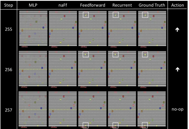
Qualitative Evaluation: Prediction video. The prediction videos of our models and base-lines are available at: https://sites.google.com/a/umich.edu/junhyuk-oh/ action-conditional-video-prediction. As seen in the videos, the proposed models make qualitatively reasonable predictions over30–500steps depending on the game. In all games, the MLP baseline quickly diverges, and the naFf baseline fails to predict the controlled object. An example of long-term predictions is illustrated in Figure 3.2. We ob-served that both of our models predict complex local translations well such as the movement of vehicles and the controlled object. They can predict interactions between objects such as collision of two objects. Since our architectures effectively extract hierarchical features using CNN, they are able to make a prediction that requires a global context. For example, in Figure 3.2, the model predicts the sudden change of the location of the controlled object (from the top to the bottom) at 257-step.

However, both of our models have difficulty in accurately predicting small objects, such as bullets in Space Invaders. The reason is that the squared error signal is small when the model fails to predict small objects during training. Another difficulty is in handling stochasticity. In Seaquest, e.g., new objects appear from the left side or right side randomly, and so are hard to predict. Although our models do generate new objects with reasonable shapes and movements (e.g., after appearing they move as in the true frames), the generated

(36)

MLP

Step naFf Feedforward Recurrent Ground Truth Action

255 256 257 é é no-op

Figure 3.2: Example of predictions over 250 steps in Freeway. The ‘Step’ and ‘Action’ columns show the number of prediction steps and the actions taken respectively. The white boxes indicate the object controlled by the agent. From prediction step 256 to 257 the controlled object crosses the top boundary and reappears at the bottom; this non-linear shift is predicted by our architectures and is not predicted by MLP and naFf. The horizontal movements of the uncontrolled objects are predicted by our architectures and naFf but not by MLP.

(37)

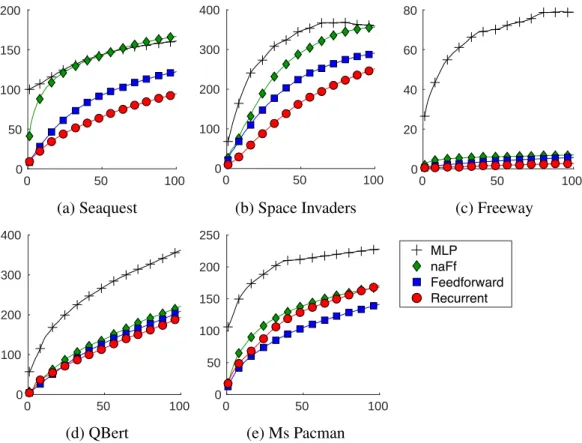
0 50 100 0 50 100 150 200 (a) Seaquest 0 50 100 0 100 200 300 400 (b) Space Invaders 0 50 100 0 20 40 60 80 (c) Freeway 0 50 100 0 100 200 300 400 (d) QBert 0 50 100 0 50 100 150 200 250 (e) Ms Pacman MLP naFf Feedforward Recurrent

Figure 3.3: Mean squared error over 100-step predictions

frames do not necessarily match the ground-truth.

Quantitative Evaluation: Squared Prediction Error. Mean squared error over 100-step predictions is reported in Figure 3.3. Our predictive models outperform the two baselines for all domains. However, the gap between our predictive models and naFf baseline is not large except for Seaquest. This is due to the fact that the object controlled by the action occupies only a small part of the image.

Qualitative Analysis of Relative Strengths and Weaknesses of Feedforward and Re-current Encoding. We hypothesize that feedforward encoding can model more precise spatial transformations because its convolutional filters can learn temporal correlations directly from pixels in the concatenated frames. In contrast, convolutional filters in recurrent encoding can learn only spatial features from the one-frame input, and the temporal context has to be captured by the recurrent layer on top of the high-level CNN features without localized information. On the other hand, recurrent encoding is potentially better for model-ing arbitrarily long-term dependencies, whereas feedforward encodmodel-ing is not suitable for long-term dependencies because it requires more memory and parameters as more frames

(38)

Feed-forward Recurrent True

(a) Ms Pacman (28×28cropped)

Feed-forward Recurrent True

(b) Space Invaders (90×90cropped)

Figure 3.4: Comparison between two encoding models (feedforward and recurrent). (a) Controlled object is moving along a horizontal corridor. As the recurrent encoding model makes a small translation error at 4th frame, the true position of the object is in the crossroad while the predicted position is still in the corridor. The (true) object then moves upward which is not possible in the predicted position and so the predicted object keeps moving right. This is less likely to happen in feedforward encoding because its position prediction is more accurate. (b) The objects move down after staying at the same location for the first five steps. The feedforward encoding model fails to predict this movement because it only gets the last four frames as input, while the recurrent model predicts this downwards movement more correctly.

are concatenated into the input.

As evidence, in Figure 3.4a we show a case where feedforward encoding is better at predicting the precise movement of the controlled object, while recurrent encoding makes a 1-2 pixel translation error. This small error leads to entirely different predicted frames after a few steps. Since the feedforward and recurrent architectures are identical except for the encoding part, we conjecture that this result is due to the failure of precise spatio-temporal encoding in recurrent encoding. On the other hand, recurrent encoding is better at predicting when the enemies move in Space Invaders (Figure 3.4b). This is due to the fact that the enemies move after 9 steps, which is hard for feedforward encoding to predict because it takes only the last four frames as input. We observed similar results showing that feedforward encoding cannot handle long-term dependencies in other games.

3.4.2 Evaluating the Usefulness of Predictions for Control

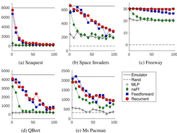
Replacing Real Frames with Predicted Frames as Input to DQN. To evaluate how useful the predictions are for playing the games, we implement an evaluation method that uses the predictive model to replace the game emulator. More specifically, a DQN controller that takes the last four frames is first pre-trained using real frames and then used to play the games based on = 0.05-greedy policy where the input frames are generated by our predictive model instead of the game emulator. To evaluate how the depth of predictions influence the quality of control, we re-initialize the predictions using the true last frames

(39)

0 50 100 0 2000 4000 6000 8000 (a) Seaquest 0 50 100 0 200 400 600 (b) Space Invaders 0 50 100 0 10 20 30 (c) Freeway 0 50 100 0 1000 2000 3000 4000 5000 (d) QBert 0 50 100 0 500 1000 1500 2000 2500 (e) Ms Pacman Emulator Rand MLP naFf Feedforward Recurrent

Figure 3.5: Game play performance using the predictive model as an emulator. ‘Emulator’ and ‘Rand’ correspond to the performance of DQN with true frames and random play respectively. The x-axis is the number of steps of prediction before re-initialization. The y-axis is the average game score measured from 30 plays.

Efficient Deep Reinforcement Learning via Planning, Generalization, and Improved Exploration