A SUMMARY OF Classification and Regression Tree WITH APPLICATION

UBT International Conference

2016 UBT International Conference

Oct 28th, 9:00 AM - Oct 30th, 5:00 PM

A SUMMARY OF Classification and Regression

Tree WITH APPLICATION

Adem Meta

Cuyahoga Community College

Follow this and additional works at:

https://knowledgecenter.ubt-uni.net/conference

Part of the

Communication Commons

, and the

Computer Sciences Commons

Recommended Citation

Meta, Adem, "A SUMMARY OF Classification and Regression Tree WITH APPLICATION" (2016).UBT International Conference. 52.

A SUMMERY OF Classification and Regression Tree

WITH APPLICATION

Adem Meta

Cuyahoga Community College, Cleveland Ohio

Abstract. Classification and regression tree (CART) is a non-parametric methodology that was introduced first by Breiman and colleagues in 1984. CART is a technique which divides populations into meaningful subgroups that allows the identification of groups of interest. CART as a classification method constructs decision trees. Depending on information that is available about the dataset, a classification tree or a regression tree can be constructed. The first part of this paper describes the fundamental principles of tree construction, pruning procedure and different splitting algorithms. The second part of the paper answers the questions why or why not the CART method should be used or not. The advantages and weaknesses of the CART method are discussed and tested in detail. Finally, CART is applied to an example with real data, using the statistical software R. In this paper some graphical and plotting tools are presented.

Keywords: Classification, Regression, Tree, Pruning, split, Goodness of fit, Algorithm.

1.

Introduction

In 1984 Breiman and colleagues introduced Classification and Regression Tress (CART). Tree methods recursively divide the data into smaller parts so as to improve the fit as best as possible. The sample space is divided into a set of small rectangles and each one is fit a model. The split of the sample space begins with two regions. Optimal splits are found over all variables at all split points. After the two regions are created then this process is repeated. The selection and stopping rules are the major components of the CART method. The stratification performed at each stage is determined by the selection rule. Then the final strata are determined by the stopping rule. The impurity of each stratum is measured after all the strata are created. Node impurity is the heterogeneity of the outcome categories within a stratum. If the outcome is categorical then Classification Trees are used. If the outcome is continuous then Regression Trees are used. Classification Trees can take different forms of categorical variables and are not limited to the analysis of categorical outcomes with two categories. The categorical variables include ordinal, indicator and non-ordinal variables. In Classification Trees there are three commonly used measures for node impurity: Gini index, misclassification error, and cross-entropy or deviance. The Gini index and cross-entropy are differentiable and easier to optimize numerically as well as being more sensitive to changes in the node probabilities. Due to this they are preferred in computer algorithms which are designed for Classification Trees and therefore used more often. In Regression Trees the measure of node impurity is least squares. Due to the lack of tests to evaluate the goodness of fit of the tree produced CARTs are not used much compared to traditional statistical methods. As well the relatively short time that CARTs have been around influences the amount of use. A statistician’s version of the popular twenty questions game is the main idea of a Classification Tree. Several questions are asked with the purpose of answering a particular research question. The trees are advantageous because of their non-parametric and non-linear nature. Using CART there do not need to be any distribution assumptions and the data generation process is treated as unknown so it does not require a functional form for the predictors. Also they

do not assume additivity of the predictors which allows them to identify complex interactions. Tree methods are one of statistical techniques that are easiest to interpret. Tree methods can be followed with little to no understanding of statistics because to a certain extent they follow the decision process humans use to make decisions. This makes them a simple to understand conceptually but yet powerful analysis tool. Nowadays in many clinical research studies there is the construction of a reliable clinical decision rule, which is used to classify new patients into clinically important categories. Examples of clinical decision rules are rules used to classify patients into groups of high or low risk categories. Clinical decision rules are used in the emergency department or out of hospital setting so that the appropriate decisions can be made regarding treatment or hospitalization.

When solving classification problems traditional statistical methods are of limited utility and hard to use. A number of reasons exist for these difficulties. First, usually there are many possible predictor variables which can make the task of variable selection difficult. Multiple comparisons cannot be effectively done with traditional statistical methods. Second, results obtained with traditional methods can be difficult to use. Third, predictor variables are commonly not well distributed. A lot of clinical variables are normally distributed with different groups of patients having different degrees of variance or variation. Fourth, the data may contain complex patterns or interactions. An example, the value of one variable (smoking or non-smoking, family history) may substantially affect the importance of another variable. Such interactions are difficult to model and become almost impossible to model when the number of interactions and variables becomes extensive.

A large data set is required for the creation of a clinical decision rule no matter which statistical methodology is being used. For every patient in the dataset the dependent variable records whether or not the patient had the condition which we hope to predict accurately in future patients. An example might be significant coronary heart disease related to the family history, age or obesity, with another possible predictor being whether or not the patient has a history of similar problems in the past. The number of possible predictor variables is quite large in most clinically important settings. The use of classification and regression tree (CART) analysis has seen an increasing interest within the last 10 years. CART analysis is a tree-building technique which is unlike traditional data analysis methods. It is best suited with the generation of clinical decision rules. CART analysis has been accepted relatively slowly because it is unlike other analysis methods. The complexity of the analysis and the difficult to use software needed for CART analysis are other important factors that have limited the general acceptability of CART.

CART analysis can be performed without a deep understanding of each of the multiple steps which are completed by the software. It is proved that CART is an effective method for creating clinical decision rules which perform as well or better than rules developed using more traditional methods. There are complex interactions between predictors which may be difficult or impossible to uncover using traditional multivariate techniques but CART often easily uncovers these complex interactions. This paper’s purpose is to provide an overview of CART methodology with an emphasis on practical uses instead of the underlying statistical theory.

CART is a robust data-analysis and data-mining tool. CART automatically searches for important relationships and patterns and quickly uncovers hidden structure even in highly complex data. The discoveries can then be used to generate accurate and reliable predictive models for applications such as targeting direct mailing, managing credit risk, profiling customers, and detecting telecommunications and credit-card fraud.

A tree explains the variation of a single response variable by splitting the data into more homogeneous groups, using combinations of explanatory variables that may be numeric and/or categorical. Each group is characterized by the number of observations in the group, the values of the explanatory variables that define it, and a typical value of the response variable. CART is accessible to both technical and nontechnical users due to it’s’ use of an intuitive Windows based interface. Behind the easy interface lies a mature theoretical foundation that distinguishes CART from other decision tree tools and methodologies.

2.

Classification Trees

One of the most used techniques in data analysis is the use of Classification Trees. They are used to predict membership of objects or cases in the classes of a categorical dependent variable from their measurements on one or more predictor variables.

Explaining or predicting responses on a categorical dependent variable is the goal of a classification tree. Due to this the techniques have much in common with the techniques used in the more traditional methods of Nonlinear Estimation and Discriminant Analysis. While the flexibility of classification tress makes them an attractive analysis option it is not recommended that they are used with the exclusion of more traditional methods. In fact, when typically, stricter theoretical and distributional assumptions of more traditional methods are men then the traditional methods may be more reliable. In such cases the traditional methods may be more reliable. However, when traditional methods fail, classification trees are an exploratory technique of last resort, which in the opinion of many researchers is more useful.

An example of a decision tree that can be helpful is the heart attack example. When a patient is admitted to a hospital with a heart attack there dozens of tests performed to obtain physiological measures such as blood pressure, heart rate, and many more. A wide array of other information such as patient’s age and medical history are also obtained. Patients can be tracked to see if they survive the heart attack for a time period, say for example at least 30 days. Advances on medical theory on heart failure and developing treatments for heart attack patients would be useful if the measurements taken directly after hospital admission can be used to identify high-risk patients, those that who may not survive at least 30 days. Breiman et al. (1984) developed a classification tree to address this problem with a simple three question decision tree. The decision tree is verbally described by the following quote, “If the patient's minimum systolic blood pressure over the initial 24-hour period is greater than 91, then if the patient's age is over 62.5 years, then if the patient displays sinus tachycardia, then and only then the patient is predicted not to survive for at least 30 days." Figure 1 below shows this decision tree.

Hierarchies of questions are asked and the final decision made depends on the answers to all the previous questions. In a similar manner, the relationship of a leaf to the tree on which it grows can be described by the hierarchy of splits of branches. This splits of branches starts from the root leading to the last branch from which the leaf hangs. One of the most basic features of a classification tree is this hierarchical nature.

A comparison to the decision making procedure employed by Discriminant Analysis illustrates the hierarchical nature of classification trees. When a traditional linear discriminant analysis is applied to the heart attack data then a set of coefficients defining the single linear combination of patient age, blood pressure, and sinus tachycardia measurements that best differentiates high risk from low risk patients are produced. Then a score for each patient on the linear discriminant function is computed as a composite of each patient’s measurements from the three predictor variables. These are then weighted by the respective discriminant function coefficients.

3.

How to split?

Splitting procedure is one of the most important concepts of the CART technique. Some information and definitions for the nodes and leaves must be provided before the splitting procedure is explained. A node is a connection point that serves as either a redistribution points or an end point for data transmissions. The node has an engineered capability to recognize, process or forward transmissions to other nodes. Starting from a root node a tree can be defined recursively as a collection of nodes along with a list of nodes known as the ‘children’. Each node in the collection is a data structure consisting of a value. There is a constraint that no node is duplicated. A definition for a tree is that it can be defined abstractly as a whole (globally) as an order tree, with a value assigned to each node. These perspectives are both useful. A tree can be mathematically analyzed as a whole. But with a tree represented as a data structure it is commonly worked with separately by each node. For example, one can analyze the parent node of a given node when looking at a tree as a whole. However, as a data structure a given node only contains the list of its children and no reference to its parent.

Though the tree all nodes can be accessed. The contents of nodes can be deleted, modified, and new elements can be created. A node tree shows the set of nodes along with the connections between them. A tree starts at the root node and then branches out to the text nodes at the lowest level of the tree. There exists a hierarchical relationship between the nodes in the node tree. The terms parent, child, and siblings are used to describe the relationships. Parent nodes have children and children nodes on the same level are called siblings (or brothers or sisters).

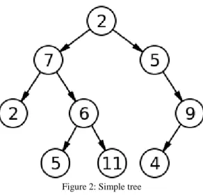
The top node is called the root node. All nodes, except the root, has exactly one parent node. A node can have any number of children. A node with no children is called a leaf.

Figure 2: Simple tree

In figure 2 above, node number 7 has two children labeled as nodes 2 and 6. Node 7 also has one parent node which in this figure is also labeled as 2 (the top). The root node (the top labeled 2) has no parent. In order to split a node into two children nodes, CART asks questions that have a ‘yes’ or ‘no’ answer. An example question would be “is coronary heart disease related with family history?”

4.

Splitting Rule and Goodness-of-Fit:

Tree construction involves making choices about three major issues. The first choice is about how splits are to be made. Which explanatory variables are to be used and where a split is to be imposed. Splitting rules define these. The second choice involves using a pruning process to determine the appropriate tree size. The third choice is to decide how to incorporate application specific costs. This can involve decisions accounting for the cost of model complexity and/or assigning varying misclassification costs.

The fitting of classification and regression trees is done through binary recursive partitioning. However, the criteria maximizing node homogeneity or minimizing node impurity is different for each of the two methods.

4.1 Gini splitting rule

The Gini index, also known as the Gini splitting rule, is the most broadly used rule. It uses the following impurity function:







t

l

p

t

k

p

t

i

(

)

(

/

)

(

/

)

















P

p

k

t

P

p

k

t

t

k

p

t

i

)

/

(

)

/

(

)

/

(

)

(

algorithm will solve the following problem:













p

k

t

P

p

k

t

P

p

k

t

)

/

(

)

/

(

)

/

(

max[

arg

algorithm will search in learning sample for the largest class and isolate it from the rest of the data. The Gini algorithm works well for noisy data.

5.

For Regression Tree:

Every regression technique contains a single response (output) variable and one or more predictor (input) variables. Output variables are reported numerically. Usual regression tree building procedure allows input variables to be a mixture of categorical and continuous variables. When each decision node in the tree contains a test on some input variable’s value a decision tree is generated. The predicted output variable values are contained by the terminal nodes of the tree. A variant of a decision tree is a regression tree. A regression tree is designed to approximate real valued functions instead of being used for classification methods. Using a process called binary recursive partitioning a regression tree is built. Binary recursive partitioning is an iterative process that splits the data into partitions or branches, and then continues to split each partition into smaller groups as the method moves up each branch. Using every binary split on every field then the algorithm begins allocating the data into the first two partitions or branches.

The split that minimizes the sum of squared deviations from the mean in the two separate partitions is selected by the algorithm. Then this splitting rule is applied to each of the new branches. The process is continued until each node reaches a user specified minimum node size and becomes a terminal node. The node is considered a terminal node even if it has not reached a minimum size if the sum of squared deviations from the mean in a node is zero.

6.

CART Advantages:

An advantage of CART is that it deals effectively with any type of data. Once the ultimate tree is obtained CART is easy to understand. CART uses conditional information effectively. CART is robust to outliers and there is no need to transform the data. CART provides the misclassification rate.

7.

CART Disadvantages:

A disadvantage of CART is that it does not help when using combinations of variables. A tree can be deceptive because a variable can be deceptive if it is masked by another. A change in the sample can give different trees therefore making tree structures unstable at times. While a tree is optimal at each split there is a chance it may not be a globally optimal. A tree can be very complicated to read when variable consist of many categories. Also there are a limited number of software programs that can be used for regression and classification tree analysis.

8.

Tree models and CART

Regression trees use a continuous response variable while classification trees involve a categorical response variable. The techniques are similar and together make up Classification and Regression Trees – CART.

Regression trees can incorporate more than one type of variable, continuous, categorical, or ordered discrete and are nonlinear predictive models. The tree model is made up of two parts. First, it is made up of recursive partition. Second, it is made up of a simple model for each cell of the partition. Each terminal node, leaf, of the tree represents a partition cell. Each cell has a simple model that only applies to that cell. By starting at the root node and asking a sequence of questions one can find which cell a unit belongs to. Each branch between nodes is the answer to a yes or no question which is imposed at each interior node. When some of the data is missing then following the tree may not lead to a leaf, however a prediction can be made by averaging all the leaves in the reached sub-tree. An example with the Boston data frame that has 506 observations and 14 variables is described below.

9.

An APPLICATION of Regression Trees for Boston Housing

Prices

Goal: Predict the price of a house in Boston, the dependent variable here, with a regression tree. Follow the directions below and enter the red commands into R.

1. Install and load the MASS library and the rpart libraries. Note: rpart uses a measure of statistical inequality called the Gini coefficient.

2. The dataset Boston is included in the rpart package, so there is no need to import data. Look at the variable names in Boston.

names(Boston)

3. Fit a regression tree model to the Boston data and get a summary of the model. In the rpart formula, "anova" indicates a regression tree.

Complexity Table

Fro m the output belo w, we can see th at at the root l evel (N ode nu mb er 1), befor e an y split s, ther e are 506 obser vations. Also, the Mean Square Error i s 84.42 and the overall d ata mean is 22. 53.

The largest tree with 39 terminal nodes has the smallest cross-validated error rate. However, this tree is too large to make predictions. The first primary split is based on the average number of rooms. If a house has less than 7 rooms, the observation goes left, otherwise it goes to the right side of the tree. The second primary split is the lower status of the population. If the number of rooms is unknown, the lower population status could be used with splitting value 9.725.

10.

Pruning

Returning to the complexity table above, the lowest error rate is a tree with 27 nodes, but because the tree with 12 terminal nodes is within one standard error of the minimum, the smaller tree with 12 terminal nodes is sufficient. Pruning the tree can be done by selecting a complexity value that is greater than that produced for the optimal tree (tree 12) but less than the complexity value for the tree above it (tree 11). Here, we need a tree with complexity parameter within 0.0048 and 0.0061.

Prune the tree with the code below:

boston.prune=prune(boston.rp,cp=0.005) plot(boston.prune,main=main="Pruned Model") text(boston.prune)

Figure 3 shows the primary split at the number of rooms per house (rm < 6.941). The second split on the left lstat seems important in terms of the models ability to partition the data to reduce the residual sums of squares. The expensive houses tend to have a higher average number of rooms. Cheaper houses have less rooms (< 7 on average) and a low status in the population with a high crime rate.

Figure 3: Tree A -- Pruning tree based on the one SE rule

10.1.

Interactive Pruning

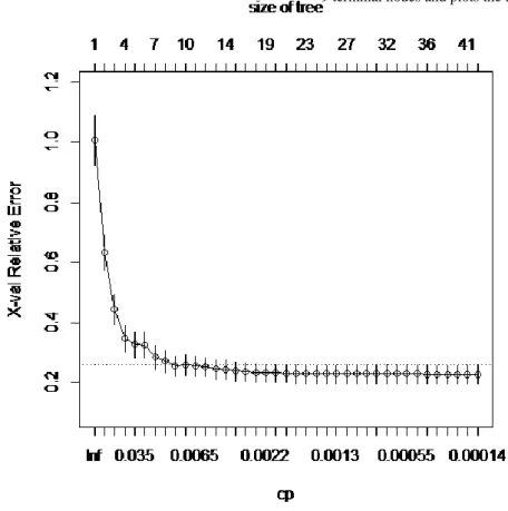
A complexity plot can aid in determining the size of the pruned tree, here, in relation to the number of terminal nodes.

plotcp(boston.rp, minline=TRUE, lty=3, col=1, upper="size")

Figure 4 shows that cross-validation suggests an optimal tree of size with between seven and fourteen terminal nodes. I chose a tree with nine terminal nodes, so we can fit this model.

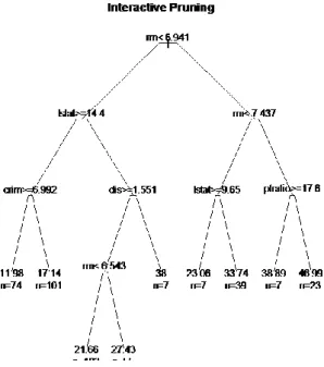
A tree can be interactively pruned in several ways. The code below prunes the tree to have only 9 terminal nodes and plots the tree.

Figure 4: Complexity plot for pruning cross-validation boston.prune.int=snip.rpart(boston.prune,toss=c(8,9,20))

plot(boston.prune.int,uniform=T,branch=0.1,main= "Interactive Pruning") text(boston.prune.int,pretty=1,use.n=T)

Notice that the interactive pruned tree below uses the variables rm, lstat, crim, dis, and ptratio for determining the splits.

Figure 5: Tree B – Results of Interactive Pruning meanvar(boston.prune.int)

11.

Predictions

Examine the predictions from both tree models using the predict function. Model 1: for Tree A

boston.pred1=predict(boston.prune) Model 2: for Tree B

boston.pred2=predict(boston.prune.int)

Compute the correlation matrix of predictions with the actual response. boston.mat.pred=cbind(Boston$medv,boston.pred1,boston.pred2) boston.mat.pred=data.frame(boston.mat.pred)

names(boston.mat.pred)=c("medv","pred.m1","pred.m2") cor(boston.mat.pred)

medv pred.m1 pred.m2 medv 1.0000000 0.9144071 0.9032262 pred.m1 0.9144071 1.0000000 0.9877725

pred.m2 0.9032262 0.9877725 1.0000000

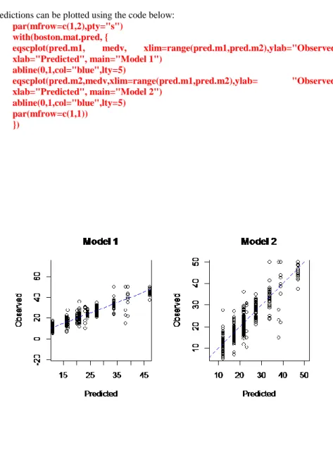
The correlation matrix above indicates that the predictions between models 1 and 2 are highly correlated with the response. Model 1 predictions are a little better than model 2 predictions. The predictions can be plotted using the code below:

par(mfrow=c(1,2),pty="s") with(boston.mat.pred, {

eqscplot(pred.m1, medv, xlim=range(pred.m1,pred.m2),ylab="Observed", xlab="Predicted", main="Model 1") abline(0,1,col="blue",lty=5) eqscplot(pred.m2,medv,xlim=range(pred.m1,pred.m2),ylab= "Observed", xlab="Predicted", main="Model 2") abline(0,1,col="blue",lty=5) par(mfrow=c(1,1)) })

The plots in Figure 6 indicate that both models are pretty good for predicting the median value of house prices in Boston. Notice that model 1 is slightly better than model 2.

What if the dataset is missing the rm variable, but we still want to predict the house price? We can create a regression tree with the average number of rooms (rm) variable removed.

boston.rp.omitRM=update(boston.rp,~.-rm) summary(boston.rp.omitRM)

…

Examine the first node.

Node number 1: 506 observations, complexity param=0.442365 mean=22.53281, MSE=84.41956

left son=2 (294 obs) right son=3 (212 obs) Primary splits:

lstat < 9.725 to the right, improve=0.4423650, (0 missing) indus < 6.66 to the right, improve=0.2594613, (0 missing) ptratio < 19.9 to the right, improve=0.2443727, (0 missing) nox < 0.6695 to the right, improve=0.2232456, (0 missing) tax < 416.5 to the right, improve=0.2017517, (0 missing) Surrogate splits:

indus < 7.625 to the right, agree=0.822, adj=0.575, (0 split) nox < 0.519 to the right, agree=0.802, adj=0.528, (0 split)

The primary split is now on lstat and the surrogate splits are indus and nox. When rm is omitted, the new model uses the competing split of the original model to make the first split.

11.1.

Examining Performance through a Test/Training Set

To get a realistic estimate of model performance, randomly divide the data into a training and test set, and then use the training set to fit the model and the test set to validate the model.

set.seed(1234) n=nrow(Boston)

Sample 80% of the data and let that be the training set and the remaining 20% is the test set. boston.samp=sample(n,round(n*.8))

bostonTrain=Boston[boston.samp,] bostonTest=Boston[-boston.samp,]

Below is a function that will produce the MSE for the previous model (re-substitution rate). testPred=function(fit, data=bostonTest){

#MSE for performance of predictor on test data testVals=data[,"medv"]

predVals=predict(fit,data[,])

sqrt(sum((testVals - predVals)^2)/nrow(data))} The MSE for the previous (pruned) model is 3.719.

[1] 3.719268

We compute the MSE for the previous model, where the original Boston dataset was used to fit the model and validate it. The MSE estimate is 3.719268, which is a resubstituting error rate. Fitting the model again to the training dataset and examining the complexity table reveals that the best model based on the one standard error rule is a tree with seven terminal nodes. The red line across the figure below represents the 1 SE rule.

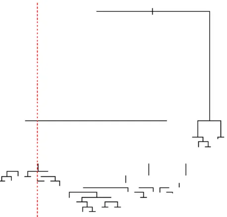
bostonTrain.rp=rpart(medv~.,data=bostonTrain,method="anova",cp=0.0001) plot(bostonTrain.rp)

abline(v=7,lty=2,col="red")

Figure 7: Regression tree with the 1 SE Rule Now we can prune and plot the training tree.

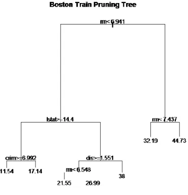
bostonTrain.prune=prune(bostonTrain.rp, cp=0.01)

plot(bostonTrain.prune, main= "Boston Train Pruning Tree") text(bostonTrain.prune)

Figure 8: Pruned Regression Tree for the Boston Training set

The computed Mean Square Error rate for the training dataset is 4.06 and the value of the MSE for the test dataset is 4.78. Clearly, these MSE values are similar, but not equal.

testPred(bostonTrain.prune, bostonTrain)

[1] 4.059407

testPred(bostonTrain.prune, bostonTest)

[1] 4.782395

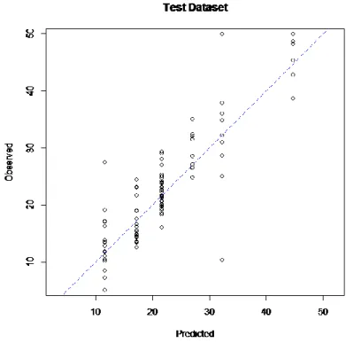
The prediction performance of the models can be examined through plots of the observed vs. predicted values.

bostonTest.pred=predict(bostonTrain.prune, bostonTest) with(bostonTest,{

cr=range(bostonTest.pred, medv)

eqscplot(bostonTest.pred, medv, xlim=cr, ylim=cr, ylab="Observed", xlab="Predicted", main="Test Dataset")

Figure 9: Scatterplot of Observed vs. Predicted prices

Figure 9 above shows that the prediction performance of the models seems to be a good indicator of the price of houses in Boston, since the data points lie close to the line.

REFERENCES

Breiman, Leo. Classification And Regression Trees. Belmont, Calif.: Wadsworth International Group, 1984. Print.

Kuhnert, P. and Venables, B. (2012). Tree-based Models II. CSIRO Mathematical and Information Sciences. [online] Available at: http://www.scribd.com/doc/18226026/An-Introduction-to-RSoftware-for-Statistical-Modelling-and-Computing-Course-Not [Accessed 27 Mar. 2016].

FINCH, H. AND SCHNEIDER, M. K.Classification Accuracy of Neural Networks vs. Discriminant Analysis, Logistic Regression, and Classification and Regression Trees Holmes and Mercedes K. Schneider. "Classification Accuracy Of Neural Networks Vs. Discriminant Analysis, Logistic Regression, And Classification And Regression Trees". Methodology 3.2 (2007): 47-57. Web.

Stine, R. (2012). Lecture 8: Classification & Regression Trees. University of Pennsylvania Data Mining Web. [online] Available at: http://www-stat.wharton.upenn.edu/~stine/mich/ DM08.pdf.

Yeh, Chyon-Hwa. "Classification And Regression Trees (CART)". Chemometrics and Intelligent Laboratory Systems 12.1 (1991): 95-96. Web.

Thernau, T., Atkinson, B. and Ripley, B. (2015). Package 'rpart'. [online] Available at: https://cran.r-project.org/web/packages/rpart/rpart.pdf [Accessed 27 May 2016].

Lesson 10: Classification/Decision Trees. (2012). Penn State STAT 557 Data Mining. The Pennsylvania State University. [online] Available at:

<https://onlinecourses.science.psu.edu/stat557/book/export/html/83>.

Regression Trees: An Overview. (2016). 1st ed. [ebook] New Zealand Digital Library: food and nutrition: University of Waikato Department of Computer Science. Available at: http://www.greenstone.org/greenstone3/nzdl?a=d&d=HASH01b184c9bb619e754e65efdc.8. pp&c=fnl2.2&sib=1&dt=&ec=&et=&p.a=b&p.s=ClassifierBrowse&p.sa= [Accessed 27 Apr. 2016].

Loh, Wei-Yin. "Fifty Years Of Classification And Regression Trees". International Statistical Review 82.3 (2014): 329-348. Web.

Lee, Seong Keon. "On Classification And Regression Trees For Multiple Responses And Its Application". Journal of Classification 23.1 (2006): 123-141. Web.

Yeh, Chyon-Hwa. "Classification And Regression Trees (CART)". Chemometrics and Intelligent Laboratory Systems 12.1 (1991): 95-96. Web.

Johnson, R. A. and D. W. Wichern. "Applied Multivariate Statistical Analysis.". Biometrics54.3 (1998): 1203. Web.