University of Kentucky University of Kentucky
UKnowledge
UKnowledge
Theses and Dissertations--Statistics Statistics
2017
Improving the Computational Efficiency in Bayesian Fitting of
Improving the Computational Efficiency in Bayesian Fitting of
Cormack-Jolly-Seber Models with Individual, Continuous,
Cormack-Jolly-Seber Models with Individual, Continuous,
Time-Varying Covariates
Varying Covariates
Woodrow BurchettUniversity of Kentucky, [email protected]
Digital Object Identifier: https://doi.org/10.13023/ETD.2017.250
Right click to open a feedback form in a new tab to let us know how this document benefits you. Right click to open a feedback form in a new tab to let us know how this document benefits you.
Recommended Citation Recommended Citation
Burchett, Woodrow, "Improving the Computational Efficiency in Bayesian Fitting of Cormack-Jolly-Seber Models with Individual, Continuous, Time-Varying Covariates" (2017). Theses and Dissertations--Statistics. 27.
https://uknowledge.uky.edu/statistics_etds/27
This Doctoral Dissertation is brought to you for free and open access by the Statistics at UKnowledge. It has been accepted for inclusion in Theses and Dissertations--Statistics by an authorized administrator of UKnowledge. For more information, please contact [email protected].
STUDENT AGREEMENT: STUDENT AGREEMENT:
I represent that my thesis or dissertation and abstract are my original work. Proper attribution has been given to all outside sources. I understand that I am solely responsible for obtaining any needed copyright permissions. I have obtained needed written permission statement(s) from the owner(s) of each third-party copyrighted matter to be included in my work, allowing electronic distribution (if such use is not permitted by the fair use doctrine) which will be submitted to UKnowledge as Additional File.
I hereby grant to The University of Kentucky and its agents the irrevocable, non-exclusive, and royalty-free license to archive and make accessible my work in whole or in part in all forms of media, now or hereafter known. I agree that the document mentioned above may be made available immediately for worldwide access unless an embargo applies.
I retain all other ownership rights to the copyright of my work. I also retain the right to use in future works (such as articles or books) all or part of my work. I understand that I am free to register the copyright to my work.
REVIEW, APPROVAL AND ACCEPTANCE REVIEW, APPROVAL AND ACCEPTANCE
The document mentioned above has been reviewed and accepted by the student’s advisor, on behalf of the advisory committee, and by the Director of Graduate Studies (DGS), on behalf of the program; we verify that this is the final, approved version of the student’s thesis including all changes required by the advisory committee. The undersigned agree to abide by the statements above.
Woodrow Burchett, Student Dr. Simon Bonner, Major Professor Dr. Constance Wood, Director of Graduate Studies
Improving the Computational Efficiency in Bayesian Fitting of Cormack-Jolly-Seber Models with Individual, Continuous, Time-Varying Covariates
DISSERTATION
A dissertation submitted in partial fulfillment of the requirements for the degree of Doctor of Philosophy in the College of Arts and Sciences
at the University of Kentucky By
Woodrow Burchett Lexington, Kentucky
Co-Directors: Dr. Simon Bonner, PhD, Professor of Statistics and Dr. Arnold Stromberg, PhD, Professor of Statistics
Lexington, Kentucky 2017
ABSTRACT OF DISSERTATION
Improving the Computational Efficiency in Bayesian Fitting of Cormack-Jolly-Seber Models with Individual, Continuous, Time-Varying Covariates
The extension of the CJS model to include individual, continuous, time-varying co-variates relies on the estimation of covariate values on occasions on which individuals were not captured. Fitting this model in a Bayesian framework typically involves the implementation of a Markov chain Monte Carlo (MCMC) algorithm, such as a Gibbs sampler, to sample from the posterior distribution. For large data sets with many missing covariate values that must be estimated, this creates a computational issue, as each iteration of the MCMC algorithm requires sampling from the full con-ditional distributions of each missing covariate value. This dissertation examines two solutions to address this problem. First, I explore variational Bayesian algorithms, which derive inference from an approximation to the posterior distribution that can be fit quickly in many complex problems. Second, I consider an alternative approx-imation to the posterior distribution derived by truncating the individual capture histories in order to reduce the number of missing covariates that must be updated during the MCMC sampling algorithm. In both cases, the increased computational efficiency comes at the cost of producing approximate inferences. The variational Bayesian algorithms generally do not estimate the posterior variance very accurately and do not directly address the issues with estimating many missing covariate val-ues. Meanwhile, the truncated CJS model provides a more significant improvement in computational efficiency while inflating the posterior variance as a result of discarding some of the data. Both approaches are evaluated via simulation studies and a large mark-recapture data set consisting of cliff swallow weights and capture histories. KEYWORDS: Mark-recapture; Bayesian Inference; Variational Bayes; Individual
Author’s signature: Woodrow Burchett
Improving the Computational Efficiency in Bayesian Fitting of Cormack-Jolly-Seber Models with Individual, Continuous, Time-Varying Covariates
By
Woodrow Burchett
Co-Director of Dissertation: Simon Bonner, PhD
Co-Director of Dissertation: Arnold Stromberg, PhD
Director of Graduate Studies: Constance Wood, PhD
ACKNOWLEDGMENTS
This dissertation would not have been possible without the leadership, guidance and constant support of my advisor, Dr. Simon Bonner. Dr. Bonner’s patience and enthusiasm are seemingly without limit and I cannot possibly thank him enough for his assistance.
I would like to express gratitude to Dr. Arnold Stromberg, Dr. Katherine Thomp-son, Dr. William Griffith, and Dr. David Westneat for serving on my committee and offering valuable suggestions and insights during this process. Thanks also to Dr. Kwok-Wai Ng for serving as the outside examiner.
I would also like to express my thanks to Dr. Matthew Schofield for initiating this project. Dr. Schofield’s enthusiasm, advice and direction were integral to the development of this dissertation.
Lastly, I would like to thank my friends and family for their support and encour-agement throughout this endeavor.
TABLE OF CONTENTS Acknowledgments . . . iii Table of Contents . . . iv List of Figures . . . vi List of Tables . . . ix Chapter 1 Introduction . . . 1 1.1 Overview . . . 1
1.2 Mark Recapture Methods . . . 6
1.3 Cormack-Jolly-Seber Model . . . 8
1.4 Continuous Covariates . . . 10
1.5 Cliff Swallows Data . . . 13
Chapter 2 Variational Bayes . . . 15
2.1 Introduction to Variational Bayesian Methods . . . 15
2.2 Application of the Mean Field Approach to the CJS Model with Con-tinuous Covariates . . . 19
Chapter 3 Improvements to the Variational Bayesian Algorithm . . . 37
3.1 Mixed Effects Model . . . 37
3.2 Modified Mean Field Approach to the CJS Model with Continuous Covariates . . . 44
3.3 Hybrid Algorithm . . . 54
3.4 Application to Cliff Swallows . . . 60
3.5 Discussion . . . 63
Chapter 4 Truncated CJS . . . 66
4.1 Introduction to Truncated CJS Model . . . 66
4.2 Truncated CJS Likelihood . . . 68
4.3 Accuracy and Precision of the Truncated CJS Model . . . 69
4.4 Simulation Study . . . 73
4.5 Application to Cliff Swallows . . . 79
Chapter 5 Conclusion . . . 88
Chapter A Appendices . . . 92
A.1 Proof of Mean Field Maximization Result . . . 92
A.2 Expected Values for MFVB Algorithm . . . 95
A.3 Derivation of Optimal Variational Densities for the MFVB Method Applied to the Mixed Effects Model . . . 97
A.4 Temporary Emigration . . . 99
Bibliography . . . 113
LIST OF FIGURES
2.1 Iterations Required for Convergence: MFVB vs MCMC . . . 29 2.2 MFVB and MCMC Parameter Estimates in Low Capture Scenario . . . 31 2.3 Simulation Results Comparing MFVB and MCMC in Low Capture Scenario 32 2.4 MFVB and MCMC Parameter Estimates in High Capture Scenario . . . 34 2.5 Simulation Results Comparing MFVB and MCMC in High Capture Scenario 35 3.1 Ormerod and Wand’s Algorithm and MCMC Parameter Estimates from
Orthodont Data . . . 39 3.2 Ormerod and Wand’s Algorithm and MCMC Parameter Estimates from
Simulated Data . . . 40 3.3 New Algorithm, Ormerod and Wand’s Algorithm, and MCMC Parameter
Estimates from Orthodont Data . . . 43 3.4 New Algorithm, Ormerod and Wand’s Algorithm, and MCMC Parameter
Estimates from Simulated Data . . . 44 3.5 Iterations Required for Convergence: MFVB vs Corrected MFVB vs MCMC 49 3.6 MFVB, Corrected MFVB, and MCMC Parameter Estimates in Low
Cap-ture Scenario . . . 51 3.7 Simulation Results Comparing MFVB, Corrected MFVB, and MCMC in
Low Capture Scenario . . . 52 3.8 MFVB, Corrected MFVB, and MCMC Parameter Estimates in High
Cap-ture Scenario . . . 53 3.9 Simulation Results Comparing MFVB, Corrected MFVB, and MCMC in
High Capture Scenario . . . 54 3.10 MFVB, Corrected MFVB, Hybrid MFVB, and MCMC Parameter
Esti-mates in Low Capture Scenario . . . 56 3.11 MFVB, Corrected MFVB, Hybrid MFVB, and MCMC Parameter
Esti-mates in High Capture Scenario . . . 57 3.12 Simulation Results Comparing MFVB, Corrected MFVB, Hybrid MFVB,
and MCMC in Low Capture Scenario . . . 58 3.13 Simulation Results Comparing MFVB, Corrected MFVB, Hybrid MFVB,
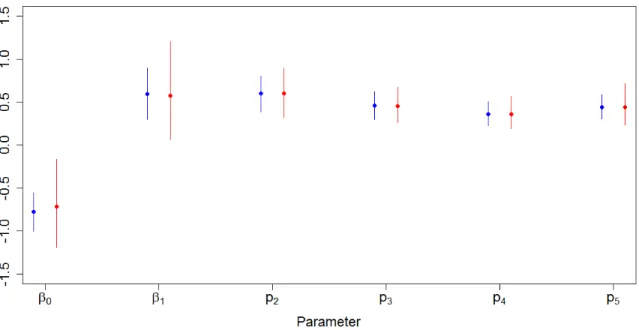
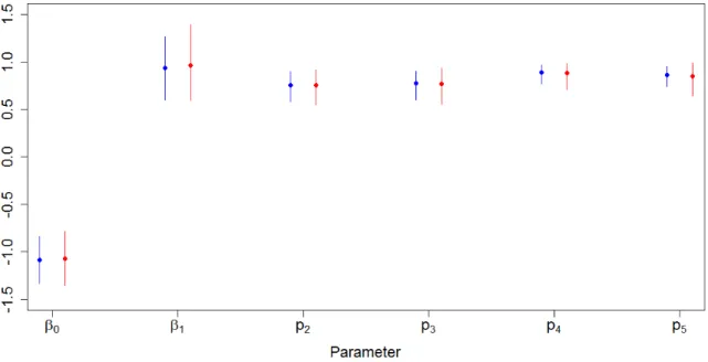
and MCMC in High Capture Scenario . . . 59 3.14 Comparison of Parameter Estimates for a Subset of Cliff Swallows Data . 61 3.15 Comparison of Parameter Estimates for Cliff Swallows Data . . . 62
4.1 KL Distances between MLEs at Different Values of k and p. . . 72 4.2 KL Distances between MLEs at Different Values of k and φ . . . 73 4.3 Parameter Estimates from the Truncated CJS Model at Different Values
of k for Simulated Data with T = 15 . . . 77 4.4 Parameter Estimates from the Truncated CJS Model at Different Values
of k for Simulated Data with T = 20 . . . 79 4.5 Estimates of Capture Parameters from the Truncated CJS Model for 8
Years of Cliff Swallows Data . . . 81 4.6 Estimates of Survival Parameters from the Truncated CJS Model for 8
Years of Cliff Swallows Data . . . 82 4.7 Estimates of Capture Parameters from the Truncated CJS Model for Cliff
Swallows Data . . . 83 4.8 Estimates of Survival Parameters from the Truncated CJS Model for Cliff
Swallows Data . . . 84 A.1 Estimates of Capture Parameters from the Truncated CJS Model for a
Single Simulated Data Set with No Temporary Emigration . . . 100 A.2 Estimates of Survival Parameters from the Truncated CJS Model for a
Single Simulated Data Set with No Temporary Emigration . . . 101 A.3 Estimates of Capture Parameters from the Truncated CJS Model for a
Single Simulated Data Set with Severe Temporary Emigration . . . 102 A.4 Estimates of Survival Parameters from the Truncated CJS Model for a
Single Simulated Data Set with Severe Temporary Emigration . . . 103 A.5 Estimates of Capture Parameters from the Truncated CJS Model for a
Single Simulated Data Set with Moderate Temporary Emigration . . . . 104 A.6 Estimates of Survival Parameters from the Truncated CJS Model for a
Single Simulated Data Set with Moderate Temporary Emigration . . . . 105 A.7 Average Estimates of Capture Parameters from the Truncated CJS Model
across 100 Simulated Data Sets with No Temporary Emigration . . . 106 A.8 Average Estimates of Survival Parameters from the Truncated CJS Model
across 100 Simulated Data Sets with No Temporary Emigration . . . 107 A.9 Average Estimates of Capture Parameters from the Truncated CJS Model
across 100 Simulated Data Sets with Severe Temporary Emigration . . . 108 A.10 Average Estimates of Survival Parameters from the Truncated CJS Model
A.11 Average Estimates of Capture Parameters from the Truncated CJS Model across 100 Simulated Data Sets with Moderate Temporary Emigration . 110 A.12 Average Estimates of Survival Parameters from the Truncated CJS Model
LIST OF TABLES
1.1 Possible probabilities assigned to an individual’s capture history . . . 10 3.1 Differences between the original MFVB algorithm and the correlation
cor-rected MFVB algorithm . . . 48 4.1 Possible probabilities assigned to individual i’s capture history . . . 68 4.2 Run times, estimated % bias, average relative standard errors, and
ef-fective samples per second when fitting the truncated CJS model (at 4 different values of k) to a data set with n = 600 and T = 15 capture occasions. . . 76 4.3 Run times, estimated % bias, average relative standard errors, and
ef-fective samples per second when fitting the truncated CJS model (at 4 different values of k) to a data set with n = 600 and T = 20 capture occasions. . . 78 4.4 Run times and effective samples per second when fitting the truncated CJS
model (at 4 different values of k) to the first 8 years of the cliff swallow data. . . 82
Chapter 1 Introduction
1.1 Overview
Mark-recapture studies have been performed by ecological researchers for over a cen-tury, beginning with Danish biologist C.G. Johannes Petersen’s study of the European plaice population in 1896 (Petersen, 1896). Since then, researchers have studied many different animal populations via mark-recapture methods, from wild Soay sheep living on an isolated Scottish island (Clutton-Brock and Pemberton, 2004) to cliff swallows nesting under bridges in the Western United States (Brown and Brown, 1996). These mark-recapture studies, which consist of capturing the animals, assigning them unique marks, and releasing them back into the population over multiple discrete capture occasions, can produce estimates of a variety of different parameters that describe the population of interest, including population size, birth rates, and survival rates. The development of methods to analyze data generated from these studies is an active area of research, incorporating many modern statistical and computational techniques such as Markov Chain Monte Carlo (Bonner and Schwarz, 2006), multiple imputa-tion (Worthington et al., 2015), Bayesian model selecimputa-tion (King et al., 2008), and the expectation-maximization (EM) algorithm (Xi et al., 2009).
Many experiments are designed to estimate the survival of individuals in a popula-tion and to identify the characteristics of the animals or environment which might im-pact an individual’s survival. Most models for studying survival from mark-recapture data are based on the Cormack-Jolly-Seber (CJS) model (Cormack, 1964; Jolly, 1965; Seber, 1965). The CJS model assigns probabilities to the individual capture histories as a function of two sets of parameters: the capture probabilities (the probability that an individual alive on a particular capture occasion is caught on that occasion) and the survival probabilities (the probability that an individual alive on a particular cap-ture occasion will also be alive on the next capcap-ture occasion). In the original model, these probabilities are allowed to vary over time, but not between individuals in the population. Additionally, the CJS model assumes that each capture occasion occurs instantaneously, marks are not mistakenly identified or lost, death or emigration is permanent, and individuals in the population behave independently of one another (Seber, 2002, page 196).
The desire for researchers to study the effects of different factors on survival and to account for possible differences in capture susceptibility led to extensions of
the CJS model being developed (Pollock, 2002). These extensions initially included models to allow for the effects of individual and environmental continuous covariates on survival and/or capture via a link function (Lebreton et al., 1992), and later those incorporating dichotomous and categorical individual covariates that change over time by way of the multi-state model (Brownie et al., 1993; Schwarz et al., 1993). The multi-state model was developed because individual, time-varying covariates are missing on capture occasions where individuals are not observed, and these missing covariate values are necessary to define the survival and/or capture probabilities. This missing data problem is solved by assuming that the covariate values follow the Markov property, which allows for the summation over all possible covariate values in the likelihood. Applying the multi-state approach to model the effect of an individual, time-varying, continuous covariate, however, would require integrating, rather that summing, over all possible missing covariate values, which results in an intractable likelihood function.
One solution to the problem of missing individual, time-varying, continuous co-variates is to discretize any such variables into discrete bins and analyze the data via the multi-state model (Nichols et al., 1992). Simple imputation techniques, such as carrying the last observation forward or taking the mean of an individual’s observed values, can also be implemented to address the issue of missing covariates. How-ever, the parameter estimates can be very biased if the imputation algorithm does not closely match the true underlying process and these imputation methods do not account for the uncertainty in covariate estimation, which will lead to artificially low standard errors (Bonner et al., 2010).
Bonner and Schwarz (2006) solved this problem by explicitly modeling the miss-ing covariates to construct a complete data likelihood. The fittmiss-ing then occurs via a Bayesian framework in which Markov Chain Monte Carlo (MCMC) algorithms are applied to generate samples from the joint posterior distribution of both the model parameters and missing covariate values. This avoids the analytically intractable integration over all possible covariate values that a maximum likelihood approach would necessitate. The specific covariate model introduced in Bonner and Schwarz (2006) assumes that the differences in covariate values from one capture occasion to the next are normally distributed, with a constant precision across all capture occasions and individuals, and that the average change between subsequent capture occasions is constant for all individuals. This is a Markov process, as was the covari-ate model assumed in the multi-stcovari-ate model. King et al. (2008) applied this technique to analyze Soay sheep data, slightly modifying the Bonner and Schwarz (2006)
co-variate model and conducting Bayesian model selection via reversible jump MCMC to probabilistically evaluate the appropriateness of different modeling assumptions. This demonstrates that the Bayesian approach to the estimation of missing contin-uous covariates is both flexible, allowing the model for the missing covariates to be easily modified to fit different real world problems, and that the assumptions made in the modeling process can be rigorously examined via Bayesian model selection techniques.
The main assumptions underlying the model for the missing covariates presented by Bonner and Schwarz (2006) are that the change in an individual’s covariate value on consecutive capture occasions is normally distributed, that the mean change be-tween subsequent capture occasions is constant across all individuals in the pop-ulation, that the variance or precision of this process is constant across sampling occasions and individuals, and that the changes are independent across sampling occasions and between individuals.
This approach, however, has limitations when it comes to analyzing very large data sets. Markov Chain Monte Carlo methods that rely on sampling repeatedly from full conditional distributions until convergence is reached often scale very poorly as the sample size increases, especially when every missing covariate value must be gener-ated on each iteration of the algorithm. This repegener-ated sampling of a potentially large number of missing covariates can make the traditional MCMC approach unfeasible, especially when the experiment was conducted over many capture occasions and indi-viduals are short lived and/or capture rates are low so that there are many occasions where individuals are not captured.
Langrock et al. (2013) attempted to address these issues by returning to the maximum likelihood framework. In particular, they finely discretized the continuous covariates to facilitate numerically integrating over the range of possible values, ex-tending the coarse binning approach found in Nichols et al. (1992). The resulting likelihood is equivalent to that of a hidden Markov model, which allowed the authors to take advantage of an efficient, recursion-based evaluation of the likelihood function. This increased efficiency in evaluating the likelihood makes maximum likelihood esti-mation feasible. Additionally, although the discretization of the continuous covariate results in the maximization of an approximate likelihood, this approximation can be made arbitrarily more accurate by more finely discretizing the covariate at the cost of computational efficiency. Langrock et al. (2013) mentioned that in the presence of two continuous, time-varying individual covariates, however, the Bayesian approach introduced by Bonner and Schwarz (2006) may be preferable, as the computational
burden for their maximum likelihood method quickly becomes untenable. Addition-ally, although Langrock et al. (2013) specifically considered mark-recapture-recovery data, the technique they introduce also applies to mark-recapture data. Note that a mark-recapture-recovery experiment is simply a mark-recapture study in which de-ceased individuals may be recovered. Also note that although the model proposed by Bonner and Schwarz (2006) was originally fit to mark-recapture data, it could just as easily be applied to mark-recapture-recovery data.
Worthington et al. (2015) approached the problem by applying the technique of multiple imputation to facilitate maximum likelihood estimation. This method begins by first modeling only the continuous covariates and then generating multiple complete sets of covariates from the fitted model. Maximum likelihood estimates can then be obtained very quickly by fitting the CJS model to each of the generated data sets with complete covariate information. This set of estimates can then be aggregated via non-parametric bootstrap techniques in order to appropriately account for the uncertainty in the estimation of the covariates. In addition to being significantly faster than the Bayesian approach introduced by Bonner and Schwarz (2006), it also avoids the computational issues present in Langrock et al. (2013) when incorporating multiple continuous covariates. The downside to the multiple imputation approach is that it relies on the assumption that the covariates are missing at random (i.e. the information contained in the capture histories is ignored when imputing the missing covariates). The authors admit that this is an unrealistic assumption, and while this method performs extremely well in the simulation results presented in Worthington et al. (2015), the simulation study only considered a covariate effect on survival. If there was a covariate effect on the capture probabilities, then the missing at random assumption would be more severely violated and I believe that substantial bias in the parameter estimates could occur.
Another approach to estimate the effects of continuous covariates on survival prob-abilities estimated from mark-recapture-recovery data was introduced by Catchpole et al. (2008). This method produces parameter estimates without the need to impute or model any missing covariates and is known as the trinomial model. The trinomial model only considers events on the occasions directly following capture occasions on which an individual was captured and the covariate measured. The likelihood, con-taining only information from those capture occasions, is then maximized to obtain parameter estimates without the need to estimate or impute any missing covariates or assume any model associated with the covariates, as all of the survival probabilities included in the likelihood will have an associated observed covariate. One drawback
of this method is the increased variance of the parameter estimates, as potentially useful information contained in individual capture histories is discarded when there is no available covariate information. This model also relies heavily on the recovery of deceased individuals present in mark-recapture-recovery data and has difficulties when covariates are associated with capture probabilities. Bonner et al. (2010) pro-vided a thorough comparison of the Bayesian missing covariate estimation and the trinomial model introduced by Catchpole et al. (2008) and found that the trinomial method can produce biased results when capture probabilities and/or sample sizes are low.
Bonner (2003) explored the implementation of an EM algorithm to address the missing data challenge when fitting the CJS model with individual, continuous, time-varying covariates. Unfortunately, the expectation step of the algorithm requires the evaluation of multi-dimensional integrals with no analytic solutions. Bonner (2003) attempted to solve this issue by approximating the expected values numeri-cally through Monte Carlo integration. However, the variability associated with the parameter estimates needed to be bootstrapped. This made the method extremely computationally demanding, as Monte Carlo integration needed to occur on every iteration of the EM algorithm which itself needed to be run multiple times to gen-erate bootstrapped variability estimates and confidence intervals. Additionally, the Monte Carlo EM approach did not perform as well as a Bayesian MCMC algorithm in simulation studies. Xi et al. (2009), while not directly addressing this problem, did successfully implement an EM algorithm to solve a missing data problem in the case of a closed population model (i.e. individuals cannot die or leave the population throughout the duration of the study) where the covariates are not time-varying.
In this dissertation, I attempt to solve the missing, individual, time-varying, con-tinuous covariate problem by exploring two very different approaches. The first in-volves abandoning the MCMC methodology for sampling from the posterior distri-bution in favor of analytical approximation (specifically, variational Bayesian tech-niques). Variational Bayesian methods provide an alternative to MCMC algorithms and have been widely applied in the field of computer science (Jordan et al., 1999; Jaakkola and Jordan, 2000; Minka, 2001; Mandt and Blei, 2014; Polatkan et al., 2015). These techniques are significantly faster and deterministic, but rely on mak-ing some assumptions about the posterior distributions to simplify the estimation process (Jordan et al., 1999; Ormerod and Wand, 2010). The idea behind variational Bayesian methodology is to replace the potentially time consuming and resource in-tensive sampling that occurs in an MCMC algorithm with an optimization problem
that is rendered tractable by making some assumptions about the underlying poste-rior distribution. The increase in speed comes at the cost of deriving inference from an approximate posterior distribution (rather than sampling from the true posterior distribution, as MCMC does) restricted by the aforementioned assumptions. Addi-tionally, this approximate posterior distribution usually underestimates the variability of the true posterior distribution (Ormerod and Wand, 2010).
My second approach relies on a different approximation to the posterior distri-bution obtained by altering the CJS likelihood to allow the truncation of capture histories, the same basic idea underlying the method described in Catchpole et al. (2008). This will reduce the number of missing covariates that must be imputed by fo-cusing on the missing data that has the most influence over the parameter estimates. To accomplish this, I truncate individual capture histories after each recapture ac-cording to a tuning parameterk. I call this approach the truncated CJS model. This method does discard some data and, as a result, produces posterior samples with higher variance than that of the true posterior distribution. As I will show, however, the posterior estimates produced when fitting this model are still unbiased and care-fully choosing the value ofk can result in an MCMC algorithm capable of generating samples from a posterior distribution that are almost indistinguishable from samples of the true posterior distribution in a fraction of the time.
The manuscript begins with an introduction to mark-recapture methods in Section 1.2, followed by the definition of the original CJS model in Section 1.3, the extension to time-varying, individual, continuous covariates in Section 1.4, and a description of the large mark-recapture data set I will analyze as an example when evaluating both of my new methods in Section 1.5. I then apply a standard variational Bayesian approach to the CJS model with individual, time-varying, continuous covariates in Chapter 2 and describe some of issues with the approximation. In Chapter 3 I produce a better variational Bayesian approximation at the cost of a large computational burden and introduce a method that combines this more accurate approximation with the faster algorithm from Chapter 2. In Chapter 4 I take a different approach and introduce the truncated CJS model, which I fit using MCMC algorithms. Finally, I conclude with some discussion about my findings in Chapter 5.
1.2 Mark Recapture Methods
Before any discussion of models or fitting algorithms can begin, I must first define the structure of data collected during mark-recapture studies. I begin by providing
a list of notation. Then, I describe how data is collected and recorded during a mark-recapture study.
Notation
The following list describes the data and parameters necessary to define the CJS model:
• Study Parameters
T = number of capture occasions
• Observed Data
n= number of individuals marked during the T capture occasions
ωi,t =
1, if individual i is captured at occasion t
0, otherwise
ωi = (ωi,1, ωi,2, . . . , ωi,T) = capture history for individual i
Ω =n by T matrix where the ith row is ωi
ai = first capture occasion on which individual iwas captured
• Model Parameters
pt= probability that an individual is captured on
sampling occasion t, given that the individual is alive
φt= probability that an individual survives to occasion
t+ 1, given that the individual is alive at occasiont
χt= probability that an individual is not observed after occasion t,
given that the individual was captured alive on occasion t Mark Recapture Data
A mark-recapture study proceeds by sampling individuals from a population over T
distinct capture occasions. This process begins on the first capture occasion, when individuals are captured, given unique marks, and released back into the population.
On subsequent capture occasions, both marked and unmarked individuals are cap-tured. On these subsequent capture occasions, the presence of previously marked individuals is noted and unmarked individuals are given a unique mark. Both previ-ously marked and unmarked individuals are then released back into the population.
At the conclusion of a mark-recapture study, n unique individuals have been recorded acrossT capture occasions. The capture histories of these individuals, after being recorded on each capture occasion, are stored in annbyT matrixΩ. Thei, t-th entry in this matrix, ωi,t is an indicator variable that takes the value 1 if individual
i was captured on occasion t and 0 if not. The ith row of Ω, ωi = (ωi,1, . . . , ωi,T),
is defined as the capture history for individual i. For example, suppose that I have data from a mark-recapture study withT = 3 capture occasions and that individuali
was first captured on the 1st capture occasion and later captured on the 3rd capture occasion. That individual’s capture history would beωi = (101).
In addition, it is common for covariates of interest to be recorded when individuals are captured. These covariates may be static, such as gender, and need only be recorded on an individual’s initial capture while others may be time varying, such as size or weight, and must be recorded on each occasion on which an individual is captured. Furthermore, these covariates can often be environmental and not related to individuals at all, such as temperature or rainfall. In the next section, I describe the original formulation of the CJS model, which does not allow for the effect of covariates. Later in Section 1.4, however, I describe the extension of the CJS model to include covariates.
1.3 Cormack-Jolly-Seber Model
Fitting a model to the mark recapture data described in the previous section allows researchers to estimate parameters of interest about the population from which the in-dividuals are sampled. The basis for most models of open population mark-recapture studies is the CJS model (Cormack, 1964; Jolly, 1965; Seber, 1965) which, in its orig-inal form, assigns probabilities to the individual capture histories as a function of two sets of parameters: capture probabilities (the probability that an individual alive on a particular capture occasion is caught on that occasion) and survival probabilities (the probability that an individual alive on a particular capture occasion will also be alive on the next capture occasion). The CJS model assigns these probabilities to capture histories conditional on each individual’s first release and assumes that individuals behave independently, sampling occasions are instantaneous, marks are
not lost or overlooked, and all death or emigration from the population is permanent. See Seber (2002, page 196) for more details on the assumptions associated with the CJS model.
To define the likelihood associated with the CJS model, I must first define some notation. Let pt represent the probability that an individual will be captured on
sampling occasion t (given that the individual is alive on occasion t), φt represent
the probability that an individual will survive until occasion t+ 1 (given that the individual is alive on occasion t), andχt represent the probability that an individual
is not observed after occasiont(given that the individual is captured alive on occasion
t). Note that χt is a function of p and φ, where p = (p1, p2, . . . , pt) and φ =
(φ1, φ2, . . . , φt), and can be defined recursively as:
χt= (1−φt) +φt(1−pt+1)χt+1, t = 1, ..., T −1
and χT = 1.
Probabilities which are functions of p, φ, and the derived quantity χ may then be assigned to each capture history.
As an example, consider the hypothetical individual mentioned in the previous section with a capture history ofω = (101). This individual’s capture history would be assigned the probability φ1(1−p2)φ2p3. The survival parameters φ1 and φ2 are
included because I know that this individual survived from capture occasion 1 to capture occasion 3. Additionally, since I know this individual was alive on capture occasions 2 and 3, I can include (1−p2) for the capture occasion on which this
indi-vidual was not captured andp3 for the capture occasion on which this individual was
captured. Note thatp1 is not included, as the probability assigned to this individual’s
capture history is conditional on the first capture.
Table 1.1 provides a complete list of all individual capture histories and the as-signed probabilities for a study with T = 3 capture occasions. The capture histories
ωi = 001 and ωi = 000 are not included in the table because they do not contribute
any information to the likelihood function due to the fact that probabilities assigned to capture histories under the CJS model condition on an individual’s first capture.
Once probabilities are assigned to every possible capture history, the likelihood for the CJS model can be written as
L(p,φ|Ω) =
n
Y
i=1
P r(ωi|ai) (1.1)
where ai denotes the occasion on which individual i was first captured. From here,
fitting can also be made extremely efficient by modeling the data in terms of sufficient statistics contained in the m-array (Burnham, 1987). The m-array summarizes the data by reporting how many individuals were captured and released at each occasion, in addition to how many of these individuals were recaptured at each of the subse-quent occasions. This information (a vector of size T −1 containing the amounts of released individuals and aT −1 byT −1 upper triangular matrix of first subsequent recaptures) is all that is required to fit the original CJS model. However, the m-array is insufficient for including individual covariates, and I will therefore consider the likelihood associated with individual capture histories for the remainder of this manuscript.
Table 1.1: Possible probabilities assigned to an individual’s capture history
Capture History Probability 111 φ1p2φ2p3 110 φ1p2χ2 101 φ1(1−p2)φ2p3 100 χ1 011 φ2p3 010 χ2 1.4 Continuous Covariates
Researchers are often interested in the effects of covariates on the parameters associ-ated with members of a population. Consider, for example, the effect of weight on the survivability of wild Soay sheep living on the Scottish island of Hirta (Clutton-Brock and Pemberton, 2004; King et al., 2008; Bonner et al., 2010). The original form of the CJS model described in Section 1.2 only allows capture and survival probabilities to vary by capture occasion, which facilitates the modeling of temporal changes in these parameters but cannot incorporate the effects of covariates. Fortunately, this model was later extended to incorporate survival and capture probabilities that are functions of covariates. Originally, these covariates were either static, such as an in-dividual’s gender, or common to all individuals, like the amount of rainfall observed before each capture occasion (Lebreton et al., 1992). Later, this model was extended to allow individual, categorical covariates via the multi-state model (Brownie et al., 1993; Schwarz et al., 1993). Bonner and Schwarz (2006) described a further exten-sion of the CJS model in which capture and survival probabilities may be functions of
continuous, time-varying, individual covariates. Fitting this model does present some challenges not present in models that include static or common covariates, however, as the values of such covariates cannot be observed on occasions on which individuals are not captured.
To solve this problem, Bonner and Schwarz (2006) modeled the distribution of the missing covariates to construct a complete data likelihood. Let zi,t represent the
covariate for individual i at time t (missing if ωi,t = 0). Bonner and Schwarz (2006)
considered this specific model for the continuous covariates: [zi,t|zi,t−1,∆t, τ]∼ N zi,t−1+ ∆t, 1 τ (1.2) where ∆t represents the average change in the covariate from capture occasion t−1
to t and τ represents the precision of the change in an individual’s covariate value between consecutive capture occasions. The main assumptions underlying this model for the missing covariates are that the change in an individual’s covariate value on consecutive capture occasions is normally distributed, that the mean change between subsequent capture occasions is constant across all individuals in the population, that the variance or precision of this process is constant across sampling occasions and individuals, and that all individual’s in the population are independent of each other.
Once the model for the covariate is defined, a link function, usually the logit, relates the covariate information to the capture or survival probabilities. For example, if I wanted to model the effect of a continuous, individual time-varying covariate on survival, then I would define the survival probabilities as:
logit(φi,t) =β0+β1zi,t
where φi,t now represents the probability that individual i survives from capture
occasionttot+ 1, given that individual iwas alive on capture occasiont. Likewise, if the capture probabilities were dependent on an individual, time-varying covariate, the probability that individual i is captured on capture occasion t, given that individual
i is alive on capture occasion t, would be denoted by pi,t. Additionally, if either the
capture or survival probabilities are modeled with respect to an individual, time-varying covariate, the probability that individual i is not observed after occasion t
will be denoted χi,t. The capture histories are then assigned probabilities which are
nearly identical to those presented in Table 1.1 (for a study with 3 capture occasions), with the only difference being the additional subscript to denote individual specific
p,φ, and χterms. The complete data likelihood can then be written as L(β,∆, τ|Ω,Z) = n Y i=1 P r(ωi|zi, ai)× T Y t=ai+1 P r(zi,t|zi,t−1) ! .
Note that the first term inside the parentheses denotes the probability associated with individuali’s capture history while the second term represents the covariate model.
Due to the presence of missing covariate data, this model is typically fit in a Bayesian framework via a Gibbs sampler, an MCMC technique, although maximum likelihood approaches have also been proposed. Two of these methods were briefly introduced in Section 1.1. The first, proposed by Langrock et al. (2013) relies on approximating the integral over all possible missing covariate values by discretizing the range of covariates, similar to the method from Nichols et al. (1992). The key difference, however, is that the range of covariate values is much more finely dis-cretized, and the likelihood is re-formulated as a hidden Markov model to make the estimation much more efficient. The other technique comes from Worthington et al. (2015) and relies on multiple imputation. First, a model is fit to the observed co-variates, ignoring any capture history data. Many complete sets of covariates are then generated by sampling missing covariate values from the fitted covariate model. Lastly, the CJS model extended to include continuous covariates is fit separately to each complete set of covariates and the parameter estimates are then aggregated us-ing a non-parametric bootstrap to properly account for uncertainty in the missus-ing covariate values (Buckland, 1984; Buckland and Garthwaite, 1991; Little and Rubin, 2014).
One of the primary reasons these maximum likelihood approaches were developed is that this particular extension of the CJS model can be computationally intensive to fit with MCMC, as missing covariate values must be imputed for every individual at every capture occasion after an individual’s first capture on which they are not captured. For extremely large data sets, this can make fitting this model via a Gibbs sampler computationally unfeasible. For example, if I were analyzing a data set in which there were 5,000 instances where individuals were not recaptured after their first capture, fitting this model via a Gibbs sampler would require sampling from 5,000 different full conditional distributions of missing covariates on each iteration of the Gibbs sampler. If I want my Gibbs sampler to generate 3 Markov chains of length 10,000, this would require sampling from the full conditional distributions of the missing covariates 150 million times. Additionally, the full conditional distribu-tions of the missing covariates are rarely in closed form, so the Gibbs sampler will
need to be generalized into a Metropolis-Hastings or other rejection sampling algo-rithm to facilitate sampling from the unknown distributions, making those 150 million sampling procedures even more computationally demanding. The new methods I de-scribe in this manuscript present new ways to reduce this computational burden by first implementing an alternative approach to MCMC, and secondly by defining a new model where fewer missing covariates need to be imputed.
1.5 Cliff Swallows Data
The ability of the two new methods I will present to improve the efficiency of the model fitting algorithms will be evaluated both via simulation studies and the analysis of an actual, large, mark-recapture data set that gives existing methods computational problems. This large mark-recapture data set comes from a 35 year study of cliff swallows led by Dr. Charles R. Brown (Brown and Brown, 1996).
To assess the performance of my two new methods, I will analyze T = 29 years of data (each year acting as a capture occasion) collected from 1984 to 2012. A total of 223,092 unique birds were marked during this period. However, we wish to incor-porate a weight covariate into our analysis, so captures that did not have a weight covariate associated with them were ignored. Note that if the individual covariates missing on capture occasions where the associated individual was captured are not missing at random, this could produce biased parameter estimates. In addition, to simplify the modeling process, only birds that were banded and observed as adults were included in the analysis. If adolescent birds were included in the analysis, we would likely need to modify the covariate model and treat survival as age category dependent. Removing adolescent birds and captures without associated weight co-variates brings the total number of birds in the data set down to n= 164,621.
Modeling the effect of an individual, time-varying covariate (weight, in this case) on capture and/or survival probabilities using the approach outlined in Bonner and Schwarz (2006) requires an MCMC algorithm to generate samples from the posterior distribution. Unfortunately, fitting this model to the cliff swallows data set requires the imputation of 1,968,151 missing covariates on each iteration of the algorithm. Gibbs sampling software packages such as JAGS (Plummer, 2003) or BUGS (Lunn et al., 2000) will therefore require substantial amounts of time and computational resources to generate samples that have converged to the posterior distribution. Later in this manuscript, I fit the CJS model with weight included as a covariate to a small
subset of this data (27,973 individuals with 56,742 missing covariate values) via JAGS, and the MCMC algorithm required 18.6 hours to reach convergence. Assuming that the run time scales linearly with the number of missing covariates, I would estimate that fitting the same model to the full cliff swallows data set would require nearly four weeks to reach convergence. Note that this estimate is quite conservative, as the additional missing covariates and capture occasions present in the complete data set would likely result in the algorithm requiring more iterations than the smaller subset to reach convergence. My goal is to reduce this computational burden by first using an alternative to MCMC algorithms that will generate estimates of the posterior distribution more quickly. Then, I will modify the likelihood so that I do not need to impute so many covariate values on each iteration of an MCMC algorithm.
Chapter 2 Variational Bayes
2.1 Introduction to Variational Bayesian Methods
Variational Bayesian methods are an alternative to MCMC for approximating pos-terior distributions and are often faster while sacrificing some accuracy. Variational Bayesian methods are widespread in computer science, particularly in machine learn-ing applications (Jordan et al., 1999; Jaakkola and Jordan, 2000; Minka, 2001; Mandt and Blei, 2014; Polatkan et al., 2015). However, this approach is starting to gain trac-tion in the statistics literature (Ormerod and Wand, 2010; Kucukelbir et al., 2015). This approach is especially helpful when large data sets render MCMC impractical, as is the situation with the CJS model extended to include individual, time-varying covariates.
Given data (y), parameters (θ), a model (p(y|θ)), and prior distributions on the parameters (p(θ)), the goal of variational Bayesian inference is to approximate the posterior distribution, p(θ|y) = p(yp|θ(y)p)(θ), with a distribution, q(θ), coming from some restricted class of distributions. The optimal variational distributionq∗(θ) is the member of the restricted class that minimizes the Kullback-Leibler distance between itself and the true posterior. The restricted class of distributions should be chosen such that finding the optimal variational distribution is tractable and the restrictions placed on the variational distributions do not depart too radically from properties of the true posterior distribution.
The critical step in finding the optimal variational distribution is the minimization of the Kullback-Leibler (K-L) distance between p(θ|y) and q(θ). The K-L distance is defined as: KL(q(θ), p(θ|y)) =Eq(θ) log q(θ) p(θ|y) = Z log q(θ) p(θ|y) q(θ)dθ.
Minimizing the K-L distance between the true posterior distribution and mem-bers of a restricted class of distributions requires algebraic manipulation such that optimizing the K-L distance forq(θ) will not require knowledge of the true posterior distribution. This is a critical step that nearly all variational Bayesian algorithms depend on. Consider that:
KL(q(θ), p(θ|y)) = Z log q(θ) p(θ|y) q(θ)dθ = Z log q(θ) p(y|θ)p(θ) q(θ)dθ+ log(p(y)) Z q(θ)dθ =−Eq(θ) log p(y|θ)p(θ) q(θ) + log(p(y)).
Note that log(p(y)) does not depend onq(θ), so minimizing the K-L distance between
q(θ) and the true posterior distribution is equivalent to maximizing
Eq(θ)
h
logp(yq|θ(θ)p)(θ)i, an expression which only depends on the the likelihood and prior distribution ofθ. This expression is often denoted byF[q] and can be interpreted as the lower bound on the marginal likelihood (Ormerod and Wand, 2010). Making the maximization of this quantity tractable is the primary concern when selecting a class of variational distributions.
Ormerod and Wand (2010) and McGrory et al. (2009) described several advan-tages of the variational Bayes methodology relative to MCMC. These advanadvan-tages include speed (particularly with regards to large data sets), results that are deter-ministic, and approximate posterior distributions in closed form. Disadvantages of these methods include the fact that they rely on distributional assumptions placed on the variational distribution, q(θ), to make the minimization of the K-L distance tractable. These distributional assumptions can be difficult or impossible to check. Additionally, the variances of the optimal variational distribution typically underes-timate the true posterior variance, sometimes radically so, depending on the assump-tions made when restricting the family of variational distribuassump-tions (Grimmer, 2010). These methods are also not nearly as general as MCMC approaches, often requiring quite a bit of analytical work, and while the MCMC algorithm will eventually sample from the true posterior distribution if run for enough iterations, variational Bayesian algorithms produce an approximation of the true posterior distribution.
Mean Field Variational Bayes
One of the most common variational approximations is the mean field variational Bayesian method (MFVB) (Ormerod and Wand, 2010). The key assumption of MFVB is that the joint variational density factorizes such that
q(θ) =
M
Y
i=1 qi(θi)
where (θ1,θ2, ...,θM) ia a partition of θ. Note that this class of variational
distri-butions can be thought of as nonparametric, as the product factorization is the only assumption made on q(θ).
The primary reason for this method’s popularity is that the mean field method’s product restriction results in tractable minimization of the Kullback-Leibler distance. A variational calculus result shows that the optimal variational distribution, denoted
q∗(θ), that achieves the minimum Kullback-Leibler distance is
q∗(θi)∝exp(E−θilogp(y,θ)), for eachi such that 1≤i≤M (2.1)
where E−θi denotes the expectation operator with respect to q−i(θ) =
Q
j6=iqj(θj).
It follows that E−θilogp(y,θ) is a function of expected values of functions of θj
(j 6=i) and parameters from the prior distributions. A detailed proof of this result is presented in Appendix A.1. Note that if a parameter or vector of parameter’s full con-ditional distribution is of known form, then that parameter or vector of parameter’s optimal variational density will also be of known form and expectations with respect to that parameter can usually be easily evaluated. The resulting optimal densities,
q∗, introduce circular dependencies which can be resolved in an iterative coordinate ascent algorithm in which the variational parameters are repeatedly, sequentially updated until convergence is reached (Ormerod and Wand, 2010). Moreover, condi-tionally conjugate priors will, by definition, lead to full conditional distributions of known form, leading to a variational Bayesian algorithm with nice analytical prop-erties (Winn and Bishop, 2005) and, coincidentally, will also lead to nice analytical properties for a Gibbs sampler (Gelman et al., 2014, pg. 280).
For illustrative purposes, I present an example of applying the mean field varia-tional Bayesian approach to a very simplistic model presented by Ormerod and Wand (2010): fitting a normal distribution to data with constant mean and variance. Sup-pose that Y1, . . . , Yn are independent normal random variables with common meanµ
and precisionτ. To ensure that the prior distributions are conditionally conjugate,µ
is assigned a normal prior with meanµ0 and precisionτ0 whileτ is assigned a gamma
prior with shape parameter α0 and rate parameter β0. Setting q(µ, τ) = q(µ)q(τ)
as the product restriction results in closed form optimal variational densities. The optimal variational density of µderived via result 2.1 is:
q∗µ(µ)∝exp(Eτ[logp(y|µ, τ) + logp(µ) + logp(τ)])
∝exp n X i=1 −(yi−µ) 2E τ[τ] 2 − (µ−µ0)2τ0 2 ! .
Completing the square shows that q∗µ(µ) is proportional to the kernel of a normal distribution: q∗µ(µ) is N nEτ[τ]¯y+τ0µ0 nEτ[τ] +τ0 ,(nEτ[τ] +τ0) −1 .
Similar derivations show that qτ∗(τ) is proportional to the kernel of a gamma distri-bution: qτ∗(τ) is G α0+ n 2, β0 + 1 2 n X i=1 Eµ[(yi−µ)2] ! .
Note that the definition of these densities are circular because the optimal variational density forµdepends on the expected value ofτ which in turn depends on an expected value with respect toµ. This interdependency is resolved with an iterative algorithm. Let µq∗(µ) represent the mean of the normally distributed variational density for µ, τq∗(µ)represent the precision of the normally distributed variational density forµ, and βq∗(τ) represent the rate parameter of the gamma distributed variational density for τ. The shape parameter of the gamma distributed variational density for τ isαq∗(τ)
= α0+ n2 and does not need to be included in the iterative algorithm as it does not
depend on the variational density ofµ. The other three variational parameters need to be included in the iterative algorithm, which I begin by initializing βq∗(τ). Note
that µq∗(µ) and τq∗(µ) could also have been initialized first. After initialization, the
algorithm can proceed:
τq∗(µ)=n α0+n2 βq∗(τ) +τ0 µq∗(µ)= n α 0+ n2 βq∗(τ) ¯ y+τ0µ0 τq−∗1(µ) βq∗(τ)=β0+ 1 2 n X i=1 (yi−µq∗(µ))2+ n τq∗(µ) ! .
Cycling through these steps leads to rapid convergence.
In this example, the resulting variational densities will be identical to the true marginal posterior distributions due to the fact that the MFVB restriction requiring independence between the variational distributions ofτ andµhappens to occur in the true posterior distribution. This is rarely the case in more complex models (Wang and Blei, 2013) and in fact the MFVB algorithm may perform quite poorly if parameters assumed to have independent variational distributions are highly correlated in the true posterior distribution, as I will demonstrate in section 3.1. This can be accounted
for by partitioning the variational densities so that highly dependent parameters are grouped together and therefore independence between them is not assumed. However, this will often make it more difficult to derive an efficient algorithm, due to the absence of closed form full conditional distributions, and also requires knowledge of which parameters will be correlated prior to fitting the model.
In Section 2.2, I apply the MFVB method to the CJS model extended to include individual, time-varying covariates, presented in Section 1.4, in an attempt to alleviate the computational burden associated with the traditional MCMC implementation of the model.
Note that there are other variational Bayesian approaches that I considered, such as nonparametric variational inference (Gershman et al., 2012) (which uses a Gaus-sian mixture to model approximate the posterior distribution) and more parametric approaches that involve specifying parametric distributions for the variational densi-ties and finding a tractable way to maximize the K-L distance. Ultimately, however, these alternative methods did not lead to an algorithm as fast, accurate, or analyti-cally convenient as the mean field approach.
2.2 Application of the Mean Field Approach to the CJS Model with Continuous Covariates
Alteration to the CJS Model with Continuous Covariates
Parameter estimates for the traditional CJS model (without covariates) can be esti-mated analytically, and for that reason, I immediately apply the variational Bayesian approach to the CJS model extended to allow for continuous, time-varying individual covariates, as described in Section 1.4. When continuous covariates are incorporated into the model, there are no closed form analytical solutions to parameter estimation and Bayesian approaches are implemented (Bonner and Schwarz, 2006). Unfortu-nately, MCMC algorithms can be computationally unfeasible for large samples and/or many capture occasions. In this section I develop a variational Bayesian algorithm to address this issue.
I use the notation described in Section 1.4 to represent the data and parameters associated with the CJS model extended to include continuous covariates. However, I define a complete data likelihood, adding a latent variable, to make deriving the vari-ational Bayesian algorithm more tractable. Recall that in Section 1.4,χi,trepresented
the probability that individual i was not observed after occasion t (given that the individual was alive on occasion t). Here, rather than summing over all possibilities
after an individual’s last capture withχ, I consider the time of an individual’s death. Letdi represent the sampling occasion on which individualiwas last alive. I can now
define a complete data likelihood that does not include anyχterms, but instead relies on the unobserved latent variable di to encapsulate the information about an
indi-vidual after it is last observed. To simplify it’s definition, I can factor the complete data likelihood contribution from each individual into two separate components: the first modeling the capture process and the second modeling survival. The capture component of the likelihood for a single individual,i, is defined as:
[ωi|di,p, fi]∝ T Y t=fi+1 (pt×1[t≤di]) ωi,t(1−p t×1[t≤di]) 1−ωi,t
where fi denotes the capture occasion on which individual iwas first captured. The
indicator function 1[t≤di] is 1 if the individual is alive at time t and 0 otherwise. I
then model di as a categorical random variable with support 1 through T:
[di|φi]∼Categorical 1−φi,1, φi,1(1−φi,2), ...,(1−φi,T−1) T−2 Y t=1 φi,t, T−1 Y t=1 φi,t
where each term in the above distribution, separated by commas, is a cell probability representing the probability that an individual dies on a particular capture occasion. The relationship between continuous covariates, such as weight or length, and survival is often of primary interest to researchers. To derive an algorithm that is easy to follow, I focus on models including a single covariate associated with survival and allow capture probabilities to vary across capture occasions. The algorithm below could be extended to include more covariates and covariates associated with capture probabilities relatively easily following the derivation of the MFVB algorithm below as a guide. I employ a logit link function to model the effect of a single, individual, time-varying covariate on survival:
logit(φi,t) = β0+β1zi,t.
Additionally, the missing covariates are modeled as in Bonner and Schwarz (2006), discussed in more detail in Section 1.4:
[zi,t|zi,t−1,∆t, τ]∼ N zi,t−1+ ∆t, 1 τ .
To complete the specification of the posterior distribution, I assign β0 and β1
inde-pendent normal priors with means µβ0 and µβ1 and precisions τβ0 and τβ1, each ∆t
priors with shape parametersαp and βp, andτ a gamma prior with shape parameter
ατ and rate parameter βτ. The hyperparameters that define the prior distributions
can be chosen such that the priors are weakly informative, which is the approach I take in the simulations and analysis to follow.
Mean Field Variational Bayesian Algorithm
I define the class of variational distributions by assuming that the posterior distri-bution of each parameter is independent of the posterior distridistri-butions of the other parameters, following the mean field variational Bayes approach introduced in Section 2.1. The only exception is that we modelq(β0, β1), allowing the twoβ parameters to
be correlated. This restriction to the class of variational distributions, combined with the new CJS likelihood presented in Section 2.2, yields a product restriction that can be written mathematically as:
q(β0, β1,p,d,∆, τ,Z) = q(β0, β1)q(τ) T Y t=1 q(pt)q(∆t) n Y i=1 q(di) Y
i,t|zi,t∈Zmis q(zi,t)
where Zmis denotes the set of all missing covariates (i.e. only the missing covariates
have variational densities). Recall that in a Bayesian framework, latent variables and missing data have posterior distributions along with the parameters in the model.
The optimal variational distributions ofd,p,∆, andτ derived by applying Equa-tion 2.1 are:
1. Variational Distribution of di
Categorical with probabilities:
q∗(di)∝
exp(Eβ0,β1,zi,li[log(1−φi,li)]), if di =li.
exp(Pdi−1
t=li Eβ0,β1,zi,t[log(φi,t)]
+Pdi
t=li+1Ep[log(1−pt)]
+Eβ0,β1,zi,di[log(1−φi,di)]), if di =li+ 1, ..., T −1.
exp(PT−1
t=li Eβ0,β1,zi,t[log(φi,t)]
+PT
t=li+1Ep[log(1−pt)]), if di =T .
0, otherwise.
2. Variational Distribution of pt
Beta with parameters:
αq∗(p t)=αp+ N X i=1 xi,t1[fi<t] ! βq∗(p t)=βp+ N X i=1 (1−xi,t)1[fi<t]P(t ≤di) !
3. Variational Distribution for ∆t
Normal with parameters:
µq∗(∆ t) = Eτ[τ]Pi|t>fi(Ez[zi,t]−Ez[zi,t−1]) +τ∆µ∆ Eτ[τ]( P i|t>fi1) +τ∆ τq∗(∆ t) = Eτ[τ] X i|t>fi 1 +τ∆
4. Variational Distribution of τ
Gamma with parameters:
αq∗(τ)=ατ + N X i=1 T X t=fi+1 1 2 βq∗(τ)=βτ + PN i=1 PT t=fi+1E∆,Z[(zi,t−zi,t−1−∆t) 2] 2
The joint variational distribution of β0 and β1 is:
q∗(β0, β1)∝exp N X i=1 T X t=fi
P(t < di)Ezi,t[log(φi,t)] + P(t=di)Ezi,t[log(1−φi,t)]
−τβ0 (β0−µβ0) 2 2 −τβ1 (β1−µβ1) 2 2
This variational distribution does not have a recognizable kernel and therefore must be approximated in some way. To resolve this issue, I have applied a Laplace ap-proximation to construct an approximate multivariate normal density for q∗(β0, β1).
Laplace approximations have been implemented previously in variational Bayesian contexts if some of the distributions are not conditionally conjugate (see Wang and Blei (2013)). Assigning logq∗(β0, β1) as the objective function in a second order
Laplace approximation results in an approximate bivariate normal distribution for
q∗(β0, β1) with variational parameters
µq∗(β 0,β1) = β0∗ β1∗ ! , Σq∗(β 0,β1) =− ∂2 ∂β2 0 logq∗(β0∗, β1∗) ∂β∂2 0∂β1 logq ∗(β∗ 0, β ∗ 1) ∂2 ∂β0∂β1 logq ∗(β∗ 0, β ∗ 1) ∂2 ∂β2 1 logq∗(β0∗, β1∗) !−1
where β0∗ and β1∗ are the values that maximize logq∗(β0, β1) and ∂2 ∂β2 0 f(β0, β1) = N X i=1 T X t=fi
−P(t≤di)Ezi,t[expit(β0+β1zi,t)×
(1−expit(β0+β1zi,t))] −τβ0 ∂2 ∂β0∂β1 f(β0, β1) = N X i=1 T X t=fi
−P(t≤di)Ezi,t[zi,texpit(β0+β1zi,t)×
(1−expit(β0+β1zi,t))] ∂2 ∂β2 1 f(β0, β1) = N X i=1 T X t=fi −P(t≤di)Ezi,t[z 2
i,texpit(β0+β1zi,t)×
(1−expit(β0+β1zi,t))]
−τβ1
and expit(x) = (1 +e−x)−1, the inverse logit or logistic function.
Similar problems also arise in deriving the variation distributions of the missing covariates. The variational distribution of any missing zi,T (i.e. an individual’s
co-variate value on the last capture occasion of the study) is a normal distribution with variational parameters
µq∗(z
i,T)= Ez[zi,T−1] + E∆[∆T] τq∗(z
i,T)= Eτ[τ]
Unfortunately, the variational distribution of a missing covariate,zi,t, witht < T has
an unrecognizable kernel:
q∗(zi,t)∝exp
−Eτ[τ] (zi,tmis)
2
+zi,tmis(E∆[∆t+1]−Ez[zi,t+1]−Ez[zi,t−1]−E∆[∆t])
+ P(t < di)Eβ0,β1[log(expit(β0 +β1zi,t))]
+ P(t=di)Eβ0,β1[log(1−expit(β0+β1zi,t))]
, t < T.
I again utilize a Laplace approximation, this time separately on each missingzi,t with
t < T. The resulting approximate variational distribution for each missing covariate,
zi,t where t < T, then follows a normal distribution with variational parameters
µq∗(z i,t) =z ∗ i,t σq2∗(z i,t) = 2Eτ[τ] + P(t≤di)Eβ0,β1[β 2 1φi,t(1−φi,t)] −1
where z∗i,t is the value that maximizes log(q∗(zi,t)).
The optimal variational densities derived above have circular dependencies with one another manifested in the expected value terms. Most of these expected val-ues are straightforward to compute. However, there are a few that do not have closed form solutions. In particular, the expected value of any function of φi,t =
(eβ0+β1zi,t)/(1 +eβ0+β1zi,t) with respect to β
0, β1, and/or a missing covariate cannot
be computed analytically. I approximate these expected values with 1st order Taylor series expansions. As with the simple normal model presented in Section 2.1, the circular dependencies can then be resolved iteratively via Algorithm 1. The expected values necessary to compute the updates in Algorithm 1 can be found in Appendix A.2.
Algorithm 1 Variational Bayesian Algorithm for the Analyses of CJS Models with Individual, Continuous, Time-Varying Covariates
1: Initialize the variational parameters ofq∗(pj),q∗(β0, β1),q∗(τ),q∗(∆j), andq∗(zi,j)
for any missing covariates.
2: whileChange in the variational parameters’ joint Euclidean norm is greater than the tolerance do
3: for i in 1 :n do
4: Update cell probabilities for q∗(di).
5: for j in 2 :T do
6: Update parameters of q∗(pj).
7: Update Laplace approximation for q∗(β0, β1).
8: Use numerical optimization to find the mean vector of the Laplace ap-proximation.
9: Use the mean vector to compute the variance-covariance matrix. 10: for i in 1 :n and do
11: for j infi :T do
12: if zi,j is missing then
13: Update the Laplace approximation for q∗(zi,j).
14: Use numerical optimization to find the mean of the Laplace
approximation.
15: Use the mean to compute the variance.
16: Update the parameters ofq∗(τ). 17: for j in 2 : T do
In practice I found that the missing covariates, updated in steps 10 through 15 of Algorithm 1, converged more slowly than the other parameters in the model due to the fact that each missing covariate’s variational density depends on both its neighbors. More precisely, the variational density of a missing covariate, zi,t, depends on both
Ez[zi,t−1] and Ez[zi,t+1] whent < T, which are functions of the variational densities of
other missing covariates. Because the variational parameters of the missing covariates are updated sequentially, missing covariate updates can potentially include parameter values from the current iteration and the previous iteration. Repeating lines 10 through 15 until the the variational parameters associated with all missing covariates converge is a technique that has proven successful in similar situations (McGrory et al., 2009) and leads to fewer total iterations of the algorithm being required to reach convergence.
Simulation Study
The two most important aspects to examine when assessing the performance of the variational Bayes algorithm are the speed of convergence and the degree of accuracy with which the optimal variational density approximates the true posterior distribu-tion. Speed of convergence is a key metric because the entire motivation behind the variational Bayesian algorithm is to present a faster alternative to the MCMC ap-proach, which struggles with large mark-recapture data sets that contain continuous, individual, time-varying covariates. The accuracy component is necessary to ensure that the resulting optimal variational density is reasonably close to the true posterior distribution.
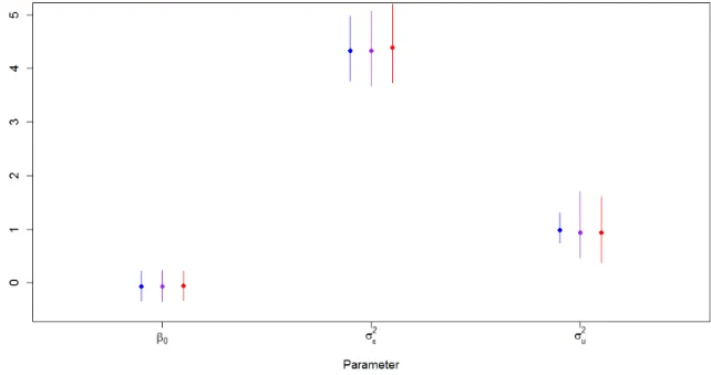
To evaluate accuracy and speed of convergence, I generated one hundred data sets with 300 individuals observed over 5 capture occasions under two sets of parameter values, one where the capture probabilities were low (0.4), and one where they were high (0.9). For the low capture scenario, I set the true parameter values as β0 =−1, β1 = 1, pt = 0.4 for all t, ∆t = 0.8 for all t, and τ = 1. I generated each individual’s
initial covariate value from a continuous uniform distribution on (−0.5,0.5), regard-less of when the individual was first captured. This set of true parameter values, in conjunction with the distribution of the initial covariate values, results in expected survival probabilities of 0.27 from fi tofi+ 1, 0.45 fromfi+ 1 tofi+ 2, 0.65fi+ 2 to
fi+ 3, and 0.80 fromfi+ 3 to fi+ 4 wherefi denotes the capture occasion on which
individuali was first captured.
Both the MCMC algorithm and the variational Bayesian algorithm were initial-ized with the same starting values. The initial value for each ∆t was generated by