Layer-wise compressive training for convolutional neural networks

04 August 2020

Repository ISTITUZIONALE

Layer-wise compressive training for convolutional neural networks / Grimaldi, Matteo; Tenace, Valerio; Calimera, Andrea. - In: FUTURE INTERNET. - ISSN 1999-5903. - 11:1(2019).

Original

Layer-wise compressive training for convolutional neural networks

Publisher: Published DOI:10.3390/fi11010007 Terms of use: openAccess Publisher copyright

(Article begins on next page)

This article is made available under terms and conditions as specified in the corresponding bibliographic description in the repository

Availability:

This version is available at: 11583/2750578 since: 2019-09-09T10:05:40Z

Article

Layer-Wise Compressive Training for Convolutional

Neural Networks

Matteo Grimaldi *, Valerio Tenace * and Andrea Calimera *

Department of Control and Computer Engineering, Politecnico di Torino, Turin 10129, Italy * Correspondence: [email protected] (M.G.); [email protected] (V.T.);

[email protected] (A.C.)

Received: 30 November 2018; Accepted: 22 December 2018; Published: 28 December 2018

Abstract:Convolutional Neural Networks (CNNs) are brain-inspired computational models designed to recognize patterns. Recent advances demonstrate that CNNs are able to achieve, and often exceed, human capabilities in many application domains. Made of several millions of parameters, even the simplest CNN shows large model size. This characteristic is a serious concern for the deployment on resource-constrained embedded-systems, where compression stages are needed to meet the stringent hardware constraints. In this paper, we introduce a novel accuracy-driven compressive training algorithm. It consists of a two-stage flow: first, layers are sorted by means of heuristic rules according to their significance; second, a modified stochastic gradient descent optimization is applied on less significant layers such that their representation is collapsed into a constrained subspace. Experimental results demonstrate that our approach achieves remarkable compression rates with low accuracy loss (<1%).

Keywords:deep learning; machine learning; neural networks on-chip; optimization

1. Introduction

Convolutional Neural Networks (CNNs) represent a class of machine learning algorithms that are able to extrapolate complex data representations from unstructured data, e.g., images, text, and audio. Starting from the astounding results obtained by Krizhevsky et al. [1] during the 2012 ImageNet competition, CNN models have been improved substantially, achieving classification accuracies that go beyond those of a human being. Today’s CNNs are considered the state-of-the-art in several application domains, such as medical diagnosis [2–4], personal home assistants [5], surveillance systems [6], and self-driving vehicles [7]. The most important factor behind the rise of CNNs, and deep learning in general, is the availability of efficient computing platforms able to speed-up the training stages, e.g., GPUs. Nonetheless, the adoption of CNNs in pervasive applications, such as those of the Internet-of-Things, is still far from being achieved. The reason is simple: the requirements of storage capacity and computational resources do not fit into low-power embedded architectures. To better grasp these concepts, let us consider the internal structure of a CNN. Figure1depicts the feature maps of the well-known VGG-16 model. It consists of several layers, each with a proper function: (i) theinput layer(red box), which produces a first transformation of the input image to be fed to the next convolutional layers; (ii) theoutput layers(gray boxes), which are perceptron-based artificial neural networks in charge of producing the final answer on the classification task; and (iii) thehidden layers, where the features extraction takes place. Figure1also shows the dimension of each layer; by summing up the contributions of all the layers, it results that even a small CNN model like the VGG-16 requires 138 MB of memory storage, and that is for weights alone. One should consider the feed-forward phase of a CNN asks for additional memory to store the partial results produced by each

layer. It is therefore clear that CNNs have to be squeezed in order to fit into architectures with few MB of memory available.

Figure 1.Topology of the VGG-16 model.

Several strategies have been proposed to shrink pre-trained CNN models. Knowledge distillation [8,9] and low rank approximation [10,11] are representative examples of non-destructive techniques. The original model serves as a reference point to generate a child model with a smaller structure and unchanged accuracy, or to generate linear-separable kernels that can be represented with a concise mathematical representation. By contrast,destructivemethods do apply a direct modification of the original CNN structure. Under this category, weights pruning [12–14] and weights quantization [15,16] are the most widely studied techniques. Inspired by the mechanisms that control and modify neural synapses in the human brain, the pruning approach is based on the idea of removing unimportant neural connections by setting their weights to zero. Quantization, instead, is used to reduce the number of bits per weight, hence the memory footprint, and thus the precision of each weight representation. Extreme quantization techniques include the possibility to quantize weights to binary [17,18] or ternary [19,20] numbers, and thus to further reduce the complexity of multiply-and-accumulate operations (replaced with simple shift operations). However, binary and ternary networks are proved to lead to huge accuracy degradations when evaluated on large datasets [21]. This is because most solutions apply a blind quantization, without taking into account how weights evolve during the training stages. In order to fill this gap, Ref. [22] introduced an efficient −σ compressive training

algorithm that accounts for weights represented in the constrained space (−σ, 0,σ). Differently from

other state-of-the-art strategies, the compressive training searches for optimalσ’s such that accuracy

degradation is minimized. However, since the accuracy loss is unconstrained, some CNN may experience large accuracy degradation.

This work improves over the original algorithm of [22] introducing a knob to control accuracy. The rationale is to apply theσ-constrained compression only on a specific sub-set of layers. An optimal

layer selection is implemented through a dedicated heuristic that quantifies thesignificanceof each layer, i.e., how the layer affects the classification performance. The resulting CNN is a hybrid model where less significant layers (those that contribute less to the inference process) are reduced with the compressive algorithm proposed in [22], whereas the most significant layers remain untouched. Experimental results demonstrate that such solution is very effective and it outperforms previous techniques achieving a better compression-accuracy trade-off.

2. Background

2.1. Overview of Training Algorithms

The termtrainingrefers to the process used to find (sub-)optimal values for all weights and biases in a neural network. The most popular training procedures make use of iterative methods that follow the derivatives of a loss function to reach a minimum cost. The loss function, here denoted with L, is the error between the output of the network and the expected one. Given~ωas the tensor that

represents all the weights in a CNN model,Lis defined as in Equation (1), with~xthe input of the CNN:

z=L(~ω,~x). (1)

Let us consider thek-th component in the input space~xk. The associated loss functionzkis the difference between~ζk, i.e., the predicted class associated to~xk, and the correct result~δk, as reported in Equation (2):

L(~ω,~x) =k~δk−~ζkk2. (2) In other words, the loss function can be seen as a measure of similarity between the outputs~ζk and~δk.

The same formulation can be extended to a batch of input tensorsB by defining the loss as the sum of all the single errors on the elements of the batch itself; this is true as errors are always positive. Hence, minimizing the sum implies minimizing each contribution. To prevent this summation to diverge, the loss function is averaged by the number of elements in the batchN as reported in Equation (3):

L(~ω) = 1

N

∑

2_{. (3)}

The stochastic gradient descent (SGD) is an iterative optimization method that can serve to minimize a loss function. It may reach the optimality of the solution when the objective function is convex and it does not stop in asaddle point, namely a point where derivatives are zero. However, when applied to non-convex functions, SGD allows reaching a local minimum. In the context of deep learning models, local minima represent a reasonable solution and a good compromise: CNNs are too complex to be handled with more sophisticated methods, whereas SGD is simple and effective. As the name suggests, the SGD implements a stochastic exploration of the solution space which is aimed to reach the optimal~ω. The search evolves following the negative slope of the objective function.

More specifically, the SGD exploits the definition of gradient, that is the vector of the first-order derivatives of the objective function as described by Equation (4). When calculated in a generic point P(v1,v2, . . . ,vN)of the optimization space, the direction of∇~PLsuggest where to move fromPto maximize the functionL. The complement−~_{∇PLheads towards lower values:}

~ ∇L= (∂L ∂w1, ∂L ∂w2, . . . , ∂L ∂wN ). (4)

Clearly, derivatives are significant in the close neighborhood ofP. Therefore, for a givenL(~ω),

the generic point~ωtshould be updated to~ωt+1accounting for a small perturbation∆ω~ as reported in

Equation (5):

~

ωt+1=ω~t+∆ω~. (5)

As∆ω~ follows−~∇PL, the loss functionLgets smaller:L(~ωt+1)<L(~ωt). It is possible to express the update as reported in Equation (6), where~ωtpoints toward the same direction as−η~∇L(~ωt), ηbeing the learning rate:

~

ωt+1=~ωt−η~∇L(~ωt). (6) According to Equation (3), the computation of∇L~ (~ωt) may result in being quite expensive depending on the cardinality of the batchB. This is reflected by Equation (7):

~

∇L(~ωt) = 1

To overcome this issue, a practical solution is to use mini-batches. Instead of computing the sum over the wholeB, each iteration just takes a sub-set ofMrandom samples as described in Equation (8), whereBMis called mini-batch. In such case, the gradient is approximated on theMcontributions:

~ ∇LM(~ωt) = 1 M_B

∑

such that the update formula becomes as in Equation (9):

~

ωt+1=~ωt−η~∇LM(~ωt). (9) Each iteration works with different mini-batches until every sample of the original batchBis visited at least once. When exhausted, the mini-batches are newly generated using different random samples fromB. This shuffling prevents any collateral biasing effect. Another property of mini-batched SGD is the ability to escape from a local minima or plateau~∇L(~ωt) =~0. Thestochasticityachieved by picking random samples can differentiate the approximated gradient~∇LM(~ωt)from~∇L(~ωt), such that these little stochastic fluctuations will possibly allow reaching a lower point.

2.2. Pruning

One of the most simple, yet effective techniques for reducing the number of weights is called pruning. It is based on the idea of removing some neural connections by setting their weights to zero. This concept is inspired by several motivations, either philosophical or empirical ones. First of all, it emulates the mechanisms that control and modify neural connections in the human brain, especially during the growth of a human being. Indeed, both artificial and biological neural networks are error-resilient: they can work if damaged, or when connections are cut off. As demonstrated in previous work, it is possible to simplify the neural network model still meeting the same original accuracy [14,23]. The second motivation is related to the redundancy of neural networks, where neurons are fully connected to all inputs, even if some connections can be useless. It may happen that a specific input does not contribute, or does not contribute in a sensible way, to a particular neuron functionality. Even worse, a connection can even alter the neuron’s functionality, for example because its weight is far from its optimal value. In this latter case, the model may stack in a local minimum where all other neurons have learned to compensate its error. In this sense, pruning can be used to jump throughout the weights space and improve the ability of the SGD method to escape from a local optimum. It also acts as an extreme form of regularization: it reduces the number of parameters in order to prevent overfitting. In this work, pruning is used as a compression strategy to reduce the model complexity.

From a practical viewpoint, each weight is a coefficient multiplying an input in a matrix-vector manner. A small weight makes a specific input quite irrelevant in the total summation; this behavior can be approximated by dropping that input. In other words, small weights can be approximated by zero-values. Generally speaking, the training algorithm sets a weighthigh(in the absolute sense) if that connection must have a strong excitatory or inhibitory effect, and hence a significant influence. Such selection can be obtained by defining a thresholdτas in the relationship in Equation (10):

ωj=

(

ωj, if|ωj| ≥τ,

0, otherwise. (10)

3. Compressive Training

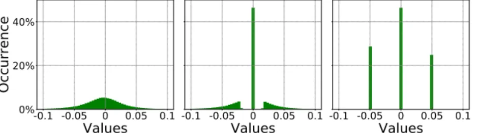
The compressive training technique is a modified version of the SGD algorithm illustrated in Section2.1. The entire procedure is based on three sequential stages. Firstly, the CNN model undergoes apreliminary training. This is accomplished through a standard training procedure during which the

weights are updated using the standard SGD algorithm. Once trained, the weights show a typical bell distribution as shown in the leftmost plot of Figure2. Secondly, an amplitude-basedweights pruning, as described in Section2.2, is applied. This stage is performed iteratively in order to gradually achieve the desired amount of sparsity, i.e., the percentage of zero-weights. Every pruning iteration is followed by a short retraining phase thus to adjust the remaining connections. The central plot in Figure2 illustrates a pruned weights distribution where almost half of the original weights are collapsed to zero. Thirdly, theσ-constrained compressionalgorithm is applied; during this phase, weights are bounded

layer-wise into the (−σ, 0,+σ) subspace; the weights distribution will then resemble the one depicted

in the rightmost plot in Figure2. It is worth noticing that each layer may have its own optimalσ.

-0.1 -0.05 0 0.05 0.1

Values

0%

20%

40%

Occurrence

-0.1 -0.05 0 0.05 0.1

Values

-0.1 -0.05 0 0.05 0.1

Values

Figure 2.Weights distribution of the second layer of AlexNet trained on CIFAR10. After the preliminary training (left), after pruning (center), after compression (right).

3.1.σ-Constrained Stochastic Gradient Descent

During the initial stage, each layerlis assigned to a preliminaryσthat is the statistical mean of the

weights distributionWl. The mean is calculated as reported in Equation (11), whereψis the number of

weights after pruning,ωiare the weights, and∆ωiis the update resulting from the back-propagation of the error function:

σ= 1 ψ ψ−1

∑

In Equation (11), positive and negative contributions can be split as shown in Equation (12):

σ= 1 ψ _ω

∑

∑

∑

∑

∑

Following the description provided in Section2.1, where∆~ω=−η∇L~ (ω~k),∆ωiis defined as in Equation (13):

∆ωi=−η∂L ∂ωi

(ω~k). (13)

At the(n+1)-th iteration, Equation (12) can be written asσ(n+1)=σn+∆σ, with∆σas reported

in Equation (14): σn= 1 ψ ψ−1

∑

∑

∑

Eachσis updated with the weighted arithmetic mean of the gradients’ components. Hence, if a

generic weight is far from its optimal value, its partial derivative would strongly affect the value ofσ.

While using the arithmetic mean for the first step represents a reasonable starting point, fine-tuningσ

The constrained space can be seen as a semi-bisector described as in Equation (15), where~sis a vector having components in the formsj=sign(ωj)and normksk=

√ ψ:

ˆ e= ~s

ksk. (15)

By expressing the non-pruned weights in their vectorized form~ω, all their possible values,

and thus the optimal solution, can be found along the tensor~ω=σn~s. However, some components of the direction could theoretically change becauseωjmight flip its sign. Therefore, the solution space is the set of all possible semi-bisectors, and the complete definition ofsj takes the form reported in Equation (16):

sj=sign(ωj+∆ωj). (16)

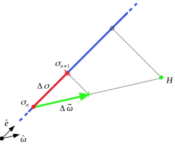
Let us assume an original 5×5 matrix pruned until only two positive weightsωx,ωyand a single negative weightωzare left. The solution space can be represented in three dimensions and becomes a semi-straight line, whose direction is~s= (1, 1,−1)T. Figure3gives a pictorial representation of the solution space. If the actual solution~ω= (ωx,ωy,ωz)T = (σn,σn,−σn)Tbelongs to the attractive valley of a minimum pointH, then−~∇L(~ω)will point towards it.

Figure 3.Visual representation of the solution space.

However,~ωcan only move along~s, i.e., ˆe. That means it is possible to find the projection of −η~∇L(~ω)on ˆeto know which is the optimal∆σas to approach as close as possible toH. This is the

ultimate sense of this algorithm: lowering or increasingσto approach the minimum point in the best

approximatedway. In fact, the scalar product Equation (17) that projects∆~ω=−η∇L~ (ω~)on ˆecan be

used to updateσn, obtaining a formulation which is similar to Equation (14):

∆σ=h~e,∆~ωi= √1 ψh~s,∆~ωi= 1 √ ψ ψ−1

∑

The difference between Equations (14) and (17) stands in the constant factor 1/√ψ, which works as a

slowing factor of the descent in the solution space. Although very effective with several deep learning models, either convolutional or recurrent, the main drawback is the lack of control on the accuracy loss. The next section introduces an accuracy-driven compressive framework which overcomes this limitation.

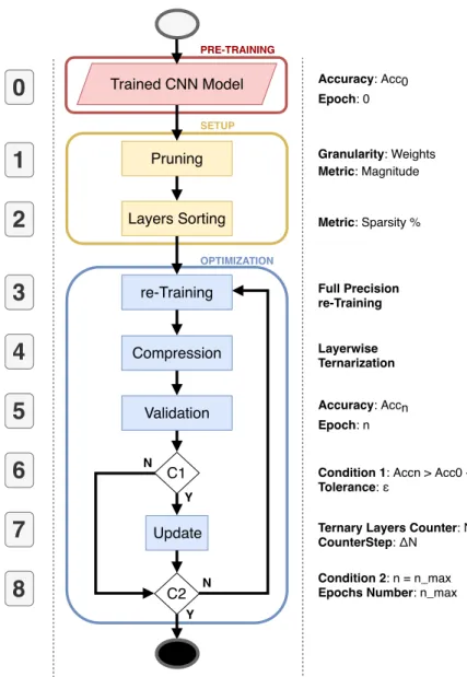
4. A Greedy Approach for Compressive Training

This section gives a step-by-step description of a new greedy strategy where layers are unevenly compressed using the compressive training algorithm. The flow is reported in Figure4. At a glance, the algorithm is composed of three main stages denoted with different colors: pre-training (light

red),setup(yellow), andoptimization(blue). The numbered boxes serve as an index for the detailed description. Trained CNN Model Pruning Layers Sorting Compression Validation C2 Update re-Training

Condition 1: Accn > Acc0 - ε Tolerance: ε

Accuracy: Acc0 Epoch: 0

Accuracy: Accn Epoch: n

Ternary Layers Counter: N += ΔN CounterStep: ΔN

C1

Condition 2: n = n_max Epochs Number: n_max Metric: Sparsity % Full Precision re-Training Layerwise Ternarization

0

1

2

3

4

5

6

7

8

Figure 4.The proposed net compression pipeline. 4.1. Pre-Training

Step 0—Trained CNN Model. The input of the proposed flow is represented by the trained model of the CNN that needs to be optimized. Our solution is designed to work on classical floating-point CNN models; however, it can be also applied to quantized CNNs. It can work equally on top of pre-trained floating-point CNN models, or onclean models, after a standard training process.

4.2. Setup

Step 1—Pruning. It consists of a standard magnitude-based pruning applied to both convolutional and fully-connected layers. The user specifies an a priori value for the desired percentage of sparsity of the net. Since such a value is unique for the entire CNN, each layer may show a different pruning percentage. This allows representing the CNN model with a non-homogeneous inter-layer sparsity. We decided to follow this direction under the assumption that each layer influences the knowledge of the CNN differently, i.e., each layer provides a specific contribution to the final prediction. For this reason, the layers do not all keep the same amount of information, but the knowledge is spread heterogeneously among the layers, and hence they keep different percentages of redundant parameters.

Step 2—Layers Sorting. It is known that some layers are more significant than others. That means the compression of less significant layers will marginally degrade the overall performance classification. The most significant layers, instead, should be preserved in their original form. As a rule of thumb, we selected theintra-layer sparsityas a measure of significance. More in detail, we argue that layers with lower intra-layer sparsity are those that play a major role in the classification process, whereas those with a higher intra-layer sparsity can be sacrificed to achieve a more compact CNN representation. In other words, we base our concept of significance on the number of activated neurons.

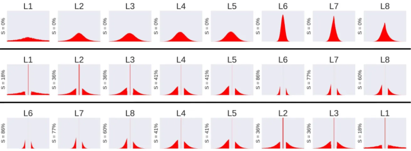
A significance-based sorted list of layers is generated at first. All layers are processed as they appear in the original model, and then pruned and sorted based on their weights distribution according to the rulehigher-sparsity first-compressed. A graphical example is reported in Figure5, where (i) the top-most pictures represent the original weight distribution of each layer (numbered L1 to L8) of the AlexNet model trained on the CIFAR10 dataset; (ii) the plots in the middle depicts the weight distribution after pruning; and (iii) the down-most plots report the layers sorted according to their significance, namely, less important layers are those with a smaller standard deviation, which is directly correlated to their sparsity.

Figure 5.AlexNet on Imagenet, layers after the sorting algorithm; the sparsity valueSis reported for each layer.

4.3. Optimization

Step 3—re-TrainingThe retraining phase is applied in order to recover the accuracy loss due to pruning. The retraining is applied after pruning at first, and then after each optimization loop.

Step 4—CompressionIt is the compressive training described in Section3. The weights are projected in a sub-dimensional space composed by just three values for each layer, i.e.,(−σ, 0,+σ),

withσdefined layer-wise.

Step 5— Validation The model is validated in order to quantify the accuracy loss due to compression, and thus to decide if it is worth continuing with further compressions. Validation is a paramount step for the greedy approach as it actually enables an accuracy-driven optimization. The accuracyAccnis evaluated and stored after each compression epochn.

Step 6—Condition 1 (C1)The accuracy recorded during then-th epoch (parameterAccn) is used to determine if the CNN model can be further compressed, as in Equation (18). The accuracy of the pre-trained model (Acc0) works as baseline, whereas the parameter erepresents the user-defined

accuracy loss tolerance:

Accn> Acc0−e. (18)

It is worth noticing that the higher the e, the higher the compression of the CNN model.

The framework takes a larger execution time for small values of e. This is due to the increased

C1 can lead to two possible branches. If Equation (18) holds true, then the algorithm goes to step 7; otherwise, the quit conditionC2 is evaluated.

Step 7—UpdateThis stage is appliedifEquation (18) is verified. The counterNindicates how many layers of the sorted list can be compressed. Each and every timeC1 is evaluated as true, andN is incremented by∆N. The latter represents another granularity knob, hence on the speed of the framework;∆Nis mainly defined by the network size: the larger the CNN model, the larger the∆N.

Step 8—Condition 2 (C2)This last condition is based on the maximum number of epochs nmax, a user-defined hyperparameter. At the n-th iteration, if more thannmax epochs are elapsed, the algorithm stops, else the flow iterates over step 3.

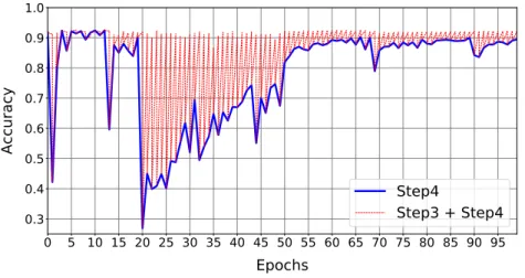
Figure6shows how accuracy evolves during the optimization loop: we report the validation’s trend during the algorithm’s epochs (blue-line), also reporting the accuracy values after both the re-Training and Compression phases (red-line). To better understand the behavior of the model during its compression, we recall that, for each loop, the algorithm first runs the retraining phase (based on a float32 back-propagation algorithm) and then a feature projection of the full precision model in the constrained solution space (this induces some accuracy drop). As the plot suggests, the performance loss is recovered within each retraining phase. The peak of loss reflects the addition of a new layer in the compressible subset list. There are layers that influence more the performance drop, but in general, after some epochs, the network reconstructs the information lost.

0 5 10 15 20 25 30 35 40 45 50 55 60 65 70 75 80 85 90 95

Epochs

0.3

0.4

0.5

0.6

0.7

0.8

0.9

1.0

Accuracy

Step4

Step3 + Step4

Figure 6.Training plot of VGG-19 architecture on CIFAR10 dataset. The plot shows the validation accuracy after the re-Training and the Compression (Step3 and Step4) with the red-line, while, with the blue-line, the validation accuracy trend on theσ-constrained solution space can be seen (after the

Compression, Step4). 5. Results

The objective of this section is to quantify the effectiveness of our compression training w.r.t. other state-of-the-art solutions. We focus on some of the most popular CNNs models and datasets.

CNN models—The adopted CNN models are trained from scratch or retrained from the Torchvisionpackage of PyTorch [24]. More specifically, we adopted the following CNNs: AlexNet [1], VGG [25], and several residual networks with increasing complexity [26].

All the models are trained and tested using PyTorch [24] (version 0.4.1). The training epochs of the compressive algorithm are fixed to 100, with a batch size of 128 and an initial learning rate of 1×10−3, which is scaled every 33 epochs by a factor of 0.1.

Datasets—CIFAR10 and CIFAR100 [27] are two large-scale image recognition benchmarks that, as their names suggest, differ for the number of available labels. Both are made up of 60,000 RGB images. The raw 32×32 data are pre-processed using a standard contrast normalization. We applied a standard data augmentation composed of a 4-pixel zero-padding with a random horizontal flip. Each dataset is equally split into 50,000 and 10,000 images for training and validation, respectively. The intersection

between training-set and validation-set is void. Tested CNNs are: AlexNet [1], VGG [25], and residual networks [26].

ImageNet (ILSVRC-2012 [28]) represents a ultra-large image dataset. Being composed of about 1.2 M images for training and over 50,000 ones for validation, it accounts for a total of 1k different classes. We followed the original data augmentation reported in [1]: the original raw images with size 256×256 are cropped into 224×224 patches with a global contrast normalization. For the training stage, the transformation is applied randomly together with a horizontal flip; during validation, a center crop manipulation is applied. AlexNet [1] and ResNet18 [26] are the two tested CNNs. 5.1. Performance

For the validation of the proposed technique, we consider the trade-off between the accuracy loss and the compression ratio. The two performance metrics are described in Equations (19) and (20). The former represents the accuracy loss and is defined as the difference in terms of accuracy percentage between the original full-precision model (ModelFP) and the compressed one (ModelC). The latter describes the compression rate defined as the ratio between the memory storage needed to save the original model’s parameters and the storage needed for saving the compressed model after the encoding. On each compressed layer, we apply the weights encoding illustrated in [22], using a 4-bit counter. In the original model, all the weights’ parameters (N0) have to be saved in 32-bit; for the compressed model, only the differentNσ_{values (one per each compressed layer) and the total number}

of weights of the full-precision layersNFPneed 32 bit precision.

AccuracyLoss [%] = Accuracy(ModelFP)−Accuracy(ModelC), (19)

CompressionRate [×] = N

0_·32 bit

NFP_·32

bit+Length(Enc)·1bit+Nσ·32bit

. (20)

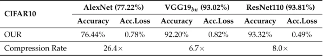
We first focus on the performance on CIFAR10 and CIFAR100 datasets withAlexNet,VGG19bn, andResNet110. Tables1and2summarize the obtained results. In both tables, the first row reports the name of the CNN model with the baseline accuracy in parentheses; the second row reports the experimental results in terms of Top-1 accuracy and accuracy loss; the last row describes the compression rate after weights encoding for each different CNN model. Obtained numbers refer to a user-defined accuracy loss of <1%. The numbers suggest not only that the accuracy constraint is successfully met, but they also indicate that very large compression rates (e.g., 26.4×for the AlexNet model) are easily achieved. This proves the adopted rationale is sound and also applicable to very complex CNN model; it allows to preserve useful information just removing redundant, or less significant, parameters on the less significant layers.

Table 1.Validation accuracy results of compressive training on CNNs trained on CIFAR10. For each CNN model, the accuracy loss (Acc.Loss) is referred to the baseline accuracy reported in parentheses.

CIFAR10 AlexNet (77.22%) VGG19bn(93.02%) ResNet110 (93.81%)

Accuracy Acc.Loss Accuracy Acc.Loss Accuracy Acc.Loss

OUR 76.44% 0.78% 92.20% 0.82% 93.32% 0.49%

Table 2.Validation accuracy results of compressive training on CNNs trained on CIFAR100. For each CNN model, the accuracy loss (Acc.Loss) is referred to the baseline accuracy reported in parentheses.

CIFAR100 AlexNet (44.01%) VGG19bn(71.95%) ResNet110 (71.14%)

Accuracy Acc.Loss Accuracy Acc.Loss Accuracy Acc.Loss

OUR 43.47% 0.54% 71.62% 0.33% 70.80% 0.34%

Compression Rate 26.4× 6.5× 7.3×

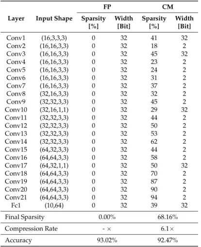
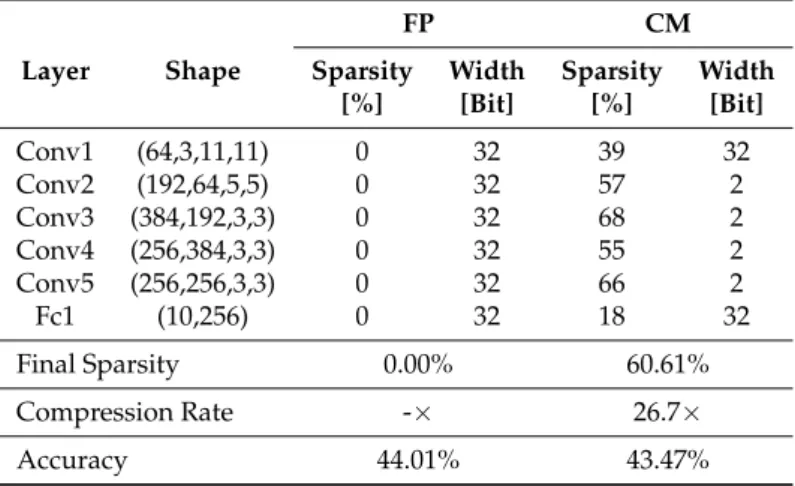
To further understand our approach, we detail two network structures before and after the greedy compressive training. Table3shows the ResNet20 architecture on CIFAR10: the two first columns show the layers ID and their input size; the next columns show the intra-layer sparsity percentage and the bit-width adopted to represent the weights, both for the full precision model (FP) and the compressed model (CM). The last rows report the sparsity of the resulting net, the compression rate w.r.t. the original model, and the final accuracy. Table4shows the same kind of metrics for AlexNet trained on CIFAR100.

Since our framework applies automatic decisions on the number of layers to compress, for each CNN and each dataset adopted, the results may change substantially, also depending on the accuracy constraint and the number of iterations run.

Table 3. Layer-wise sparsity and width before (Full Precision) and after the compressive greedy technique (Compressed Model) application on ResNet20 architecture (CIFAR10). Considering that convolutional layers have input shape(n,cin,kh,kw), and fully-connected layers have input shape (n,cin), wherekhandkware respectively the height and width of input planes in pixels, whilecin denotes the number of input channels andnthe batch size.

FP CM

Layer Input Shape Sparsity Width Sparsity Width

[%] [Bit] [%] [Bit] Conv1 (16,3,3,3) 0 32 41 32 Conv2 (16,16,3,3) 0 32 18 2 Conv3 (16,16,3,3) 0 32 45 32 Conv4 (16,16,3,3) 0 32 23 2 Conv5 (16,16,3,3) 0 32 24 2 Conv6 (16,16,3,3) 0 32 31 2 Conv7 (16,16,3,3) 0 32 37 2 Conv8 (32,16,3,3) 0 32 32 2 Conv9 (32,32,3,3) 0 32 45 2 Conv10 (32,16,1,1) 0 32 29 32 Conv11 (32,32,3,3) 0 32 44 2 Conv12 (32,32,3,3) 0 32 50 2 Conv13 (32,32,3,3) 0 32 53 2 Conv14 (32,32,3,3) 0 32 62 2 Conv15 (64,32,3,3) 0 32 44 2 Conv16 (64,64,3,3) 0 32 58 2 Conv17 (64,32,1,1) 0 32 50 32 Conv18 (64,64,3,3) 0 32 70 2 Conv19 (64,64,3,3) 0 32 87 2 Conv20 (64,64,3,3) 0 32 90 2 Conv21 (64,64,3,3) 0 32 94 2 Fc1 (10,64) 0 32 39 32 Final Sparsity 0.00% 68.16% Compression Rate -× 6.1× Accuracy 93.02% 92.47%

Table 4. Layer-wise sparsity and width before (Full Precision) and after the compressive greedy technique (Compressed Model) application on AlexNet architecture (CIFAR100). Considering that convolutional layers have input shape(n,cin,kh,kw), and fully-connected layers have input shape (n,cin), wherekhandkware, respectively, the height and width of input planes in pixels, whilecin denotes the number of input channels andnthe batch size.

FP CM

Layer Shape Sparsity Width Sparsity Width

[%] [Bit] [%] [Bit] Conv1 (64,3,11,11) 0 32 39 32 Conv2 (192,64,5,5) 0 32 57 2 Conv3 (384,192,3,3) 0 32 68 2 Conv4 (256,384,3,3) 0 32 55 2 Conv5 (256,256,3,3) 0 32 66 2 Fc1 (10,256) 0 32 18 32 Final Sparsity 0.00% 60.61% Compression Rate -× 26.7× Accuracy 44.01% 43.47%

5.2. Comparison with the State-of-the-Art

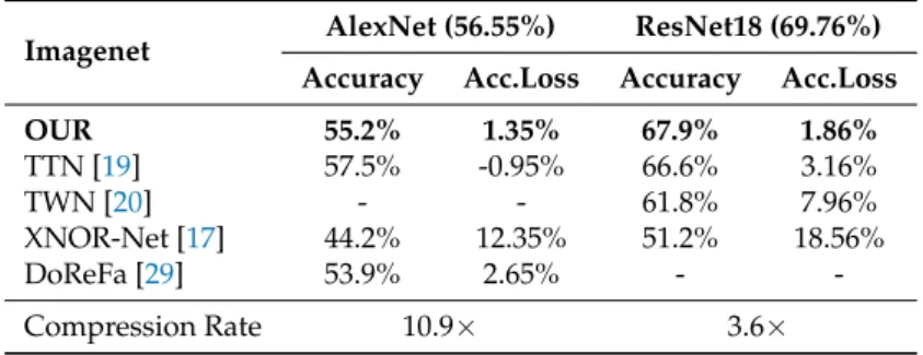
The analysis includes some of the most popular works on aggressive CNN compression: Xnor-Net[17], by Rastegari et al., where both filters and feature maps are optimized in a binary space; Ternary Weights Network(TWN) [20] where Li and Liu et al. overcame the binary solution space adding the zero value as third quantized instance;Trained Ternary Quantization(TTQ) [19], where Zhu et al. propose a new ternary quantization procedure able to use just 2-bit weights (with relative scaling factors) during CNN inference; DoReFa-Net[29], where Zhou el al. explored hybrid CNNs with different quantization widths for weights, gradients, and activations type with binary weights and 32-bit activations; we focus on the 1-32-32 DoReFa-Netin particular. For all the comparisons, the baseline is the accuracy obtained with full-precision models found in the PyTorch repository. In the following text, we use the accuracy loss as the main metric for comparison. Indeed, the results reported in the previous works do implement any encoding scheme and comparing the compressive rates might result in being quite unfair.

Let us first consider the results on the CIFAR10 dataset. The first row in Table5describes the ResNet20 and ResNet56 baseline accuracies; each column reports the obtained results. For the first CNN model, our technique is able to outperform TTN’s solution with just 0.55% of accuracy loss, whereas, for the ResNet56, the solution is closer to the baseline. However, for both networks, we set up the accuracy toleranceeat 1%, reaching a considerable compression rate (6.1×and 6.9×).

Table6reports the experimental results obtained with the Imagenet dataset. We can see that, for AlexNet, the best solution is that achieved with TTN. In fact, they claim to be able to improve over full precision model. Their solution consists of a ternary weights CNN model (with relative scaling factors), except for the first and last layers, which are kept on float32 precision. Our solution outperforms all the other solutions, e.g., a 12.35% delta w.r.t. XNOR-Net. On the other hand, with the ResNet18 architecture, our model is able to outperform all considered state-of-the-art techniques, reaching just 1.86% of accuracy loss. For this set of experiments, considering the 1k-labels dataset complexity, we fixed the accuracy toleranceeat 2%, reaching compression rates of 10.9×for AlexNet

Table 5.Validation accuracy results of compressive training on CNNs trained on CIFAR10, comparison with respect to TTN work. For each CNN model, the accuracy loss (Acc.Loss) is referred to the baseline accuracy reported in parentheses. The compression rates are considered just for our solution.

CIFAR10 ResNet20 (93.02%) ResNet56 (93.65%)

Accuracy Acc.Loss Accuracy Acc.Loss

OUR 92.47% 0.55% 93.04% 0.61%

TTN [19] 91.13% 1.89% 93.56% 0.09%

Compression Rate 6.1× 6.9×

Table 6.Validation accuracy results of compressive training on CNNs trained on Imagenet, comparison with respect to other compressive approaches. For each CNN model, the accuracy loss (Acc.Loss) is referred to the baseline accuracy reported in parentheses. The compression rates are considered just for our solution.

Imagenet AlexNet (56.55%) ResNet18 (69.76%)

Accuracy Acc.Loss Accuracy Acc.Loss

OUR 55.2% 1.35% 67.9% 1.86% TTN [19] 57.5% -0.95% 66.6% 3.16% TWN [20] - - 61.8% 7.96% XNOR-Net [17] 44.2% 12.35% 51.2% 18.56% DoReFa [29] 53.9% 2.65% - -Compression Rate 10.9× 3.6×

6. Conclusions and Future Works

In this paper, we presented a layer-wise compressive training tool that is able to significantly squeeze CNN structures with minimal accuracy drops (below 1%). Our approach leverages a heuristic that identifies the most appropriate layers to be compressed. This allows for reaching a sub-optimal combination of mixed representations that obeys user-defined accuracy constraints. Experimental results show that the proposed solution overcomes the limitation of a blind pruning, thus providing a smart optimization flow for an effective deployment of CNNs on devices with low storage capacity. Despite the remarkable achievements shown in the paper, there is much room for improvement. First, the sparsity-based empirical rule used to drive the layer-by-layer compression can be expanded with additional parameters that give a more accurate estimation of the accuracy drop. That would help to improve the accuracy-compression trade-off. Second, the execution time of the compression loop can be reduced by lowering the number of retraining epochs. There exists an optimal setting of the hyper-parameters used in the flow, e.g.,C1 andC2, which is a function of the dataset adopted and the CNN under design. Finally, the use of quantization, e.g., fixed-point weights, represents an orthogonal knob that brings additional savings in terms of both memory storage and computational resources.

Author Contributions:All the authors listed in the first page made substantial contributions to the design and implementation of the research, to the analysis of the results and to the writing of the manuscript.

Funding:This research was co-funded by Compagnia di San Paolo. Conflicts of Interest:The authors declare no conflict of interest. References

1. Krizhevsky, A.; Sutskever, I.; Hinton, G.E. Imagenet classification with deep convolutional neural networks. In Proceedings of the 25th International Conference on Neural Information Processing Systems, Lake Tahoe, Nevada, 3–6 December 2012; pp. 1097–1105.

2. Poplin, R.; Varadarajan, A.V.; Blumer, K.; Liu, Y.; McConnell, M.V.; Corrado, G.S.; Peng, L.; Webster, D.R. Predicting cardiovascular risk factors from retinal fundus photographs using deep learning. arXiv2017, arXiv:1708.09843.

3. Milletari, F.; Navab, N.; Ahmadi, S.A. V-net: Fully convolutional neural networks for volumetric medical image segmentation. In Proceedings of the 2016 Fourth International Conference on 3D Vision (3DV), Stanford, CA, USA, 25–28 October 2016; pp. 565–571.

4. Litjens, G.; Kooi, T.; Bejnordi, B.E.; Setio, A.A.A.; Ciompi, F.; Ghafoorian, M.; Van Der Laak, J.A.; Van Ginneken, B.; Sánchez, C.I. A survey on deep learning in medical image analysis.Med. Image Anal.2017, 42, 60–88. [CrossRef] [PubMed]

5. Schlüter, J.; Grill, T. Exploring Data Augmentation for Improved Singing Voice Detection with Neural Networks. In Proceedings of the 16th International Society for Music Information Retrieval Conference (ISMIR 2015), Malaga, Spain, 26–30 October 2015; pp. 121–126.

6. Wang, J.; Chen, Y.; Hao, S.; Peng, X.; Hu, L. Deep learning for sensor-based activity recognition: A survey. Pattern Recognit. Lett.2018, in press. [CrossRef]

7. Bojarski, M.; Del Testa, D.; Dworakowski, D.; Firner, B.; Flepp, B.; Goyal, P.; Jackel, L.D.; Monfort, M.; Muller, U.; Zhang, J.; et al. End to end learning for self-driving cars. arXiv2016, arXiv:1604.07316.

8. Hinton, G.; Vinyals, O.; Dean, J. Distilling the knowledge in a neural network. arXiv2015, arXiv:1503.02531. 9. Ba, J.; Caruana, R. Do deep nets really need to be deep? arXiv2014, arXiv:1312.6184.

10. Rigamonti, R.; Sironi, A.; Lepetit, V.; Fua, P. Learning separable filters. In Proceedings of the IEEE Conference on Computer Vision and Pattern Recognition, Portland, OR, USA, 23–28 June 2013; pp. 2754–2761. 11. Jaderberg, M.; Vedaldi, A.; Zisserman, A. Speeding up convolutional neural networks with low rank

expansions. arXiv2014, arXiv:1405.3866.

12. LeCun, Y.; Denker, J.S.; Solla, S.A. Optimal brain damage. InAdvances in Neural Information Processing Systems; Morgan Kaufmann Publishers Inc.: San Francisco, CA, USA, 1990; pp. 598–605.

13. Li, H.; Kadav, A.; Durdanovic, I.; Samet, H.; Graf, H.P. Pruning filters for efficient convnets. arXiv2016, arXiv:1608.08710.

14. Han, S.; Mao, H.; Dally, W.J. Deep compression: Compressing deep neural networks with pruning, trained quantization and huffman coding. arXiv2015, arXiv:1510.00149.

15. Gong, Y.; Liu, L.; Yang, M.; Bourdev, L. Compressing deep convolutional networks using vector quantization. arXiv2014, arXiv:1412.6115.

16. Wu, J.; Leng, C.; Wang, Y.; Hu, Q.; Cheng, J. Quantized convolutional neural networks for mobile devices. In Proceedings of the IEEE Conference on Computer Vision and Pattern Recognition, Las Vegas, NV, USA, 27–30 June 2016; pp. 4820–4828.

17. Rastegari, M.; Ordonez, V.; Redmon, J.; Farhadi, A. Xnor-net: Imagenet classification using binary convolutional neural networks. In Proceedings of the European Conference on Computer Vision, Amsterdam, The Netherlands, 11–14 October 2016; pp. 525–542.

18. Courbariaux, M.; Bengio, Y.; David, J.P. Binaryconnect: Training deep neural networks with binary weights during propagations. arXiv2015, arXiv:1511.00363.

19. Zhu, C.; Han, S.; Mao, H.; Dally, W.J. Trained ternary quantization. arXiv2016, arXiv:1612.01064. 20. F. Li, B. Zhang, B.L. Ternary Weight Networks. arXiv2016, arXiv:1605.04711.

21. Hashemi, S.; Anthony, N.; Tann, H.; Bahar, R.I.; Reda, S. Understanding the impact of precision quantization on the accuracy and energy of neural networks. In Proceedings of the Design, Automation & Test in Europe Conference & Exhibition (DATE), Lausanne, Switzerland, 27–31 March 2017; pp. 1474–1479.

22. Grimaldi, M.; Pugliese, F.; Tenace, V.; Calimera, A. A compression-driven training framework for embedded deep neural networks. In Proceedings of the Workshop on INTelligent Embedded Systems Architectures and Applications, Turin, Italy, 4 October 2018; pp. 45–50.

23. Han, S.; Pool, J.; Tran, J.; Dally, W. Learning both weights and connections for efficient neural network. arXiv2015, arXiv:1506.02626.

24. Paszke, A.; Gross, S.; Chintala, S.; Chanan, G.; Yang, E.; DeVito, Z.; Lin, Z.; Desmaison, A.; Antiga, L.; Lerer, A. Automatic differentiation in PyTorch. In Proceedings of the 31st Conference on Neural Information Processing Systems (NIPS 2017), Long Beach, CA, USA, 4–9 December 2017.

25. Simonyan, K.; Zisserman, A. Very deep convolutional networks for large-scale image recognition.arXiv2014, arXiv:1409.1556.

26. He, K.; Zhang, X.; Ren, S.; Sun, J. Deep residual learning for image recognition. In Proceedings of the IEEE Conference on Computer Vision and Pattern Recognition, Las Vegas, NV, USA, 27–30 June 2016; pp. 770–778. 27. Krizhevsky, A.; Hinton, G.Learning Multiple Layers of Features From Tiny Images; Technical Report; University

of Toronto: Toronto, ON, Canada, 2009.

28. Deng, J.; Dong, W.; Socher, R.; Li, L.J.; Li, K.; Fei-Fei, L. ImageNet: A Large-Scale Hierarchical Image Database. In Proceedings of the 2009 IEEE Conference on Computer Vision and Pattern Recognition, Miami, FL, USA, 20–25 June 2009.

29. Zhou, S.; Wu, Y.; Ni, Z.; Zhou, X.; Wen, H.; Zou, Y. Dorefa-net: Training low bitwidth convolutional neural networks with low bitwidth gradients.arXiv2016, arXiv:1606.06160.

c

2018 by the authors. Licensee MDPI, Basel, Switzerland. This article is an open access article distributed under the terms and conditions of the Creative Commons Attribution (CC BY) license (http://creativecommons.org/licenses/by/4.0/).