The role of physics based models for simulating runoff responses to rural land management scenarios

(1)

The role of physics based models for

simulating runoff responses to rural land

management scenarios

by

Caroline Elizabeth Ballard

A Thesis submitted for the degree of Doctor of Philosophy from

Imperial College London

2011

Department of Civil and Environmental Engineering

Imperial College London

(2)

(3)

Abstract

Recent floods in the UK have focused attention on the effects of rural land use and land management change on flood risk. Over recent decades agricultural intensification has been widespread across the uplands of the UK, with increases in stocking density, ploughing, reseeding and drainage of fields, use of heavy machinery, and the removal of trees from the landscape. A key scientific question is whether or not these changes in land use and land management in the uplands are increasing flood frequency and magnitude. Although land use and land management changes have been observed to change local surface runoff, attempts to isolate these responses at the catchment scale have failed due to limitations of data sets and modelling capability. While hydrological modelling is a well advanced field of science, a key methodological challenge that remains is how to upscale information about local scale changes.

This Thesis evaluates the role of physics based hydrological models for upscaling local scale hydrological process knowledge and data to catchment scale flood flow responses. A model upscaling procedure that aims to quantify the changes in peak flows at multiple scales related to localised land use management changes is presented. The procedure divides the catchment into a number of runoff generating elements, which are each classified based on soil types and land management. For each runoff generating element, a physics based model is developed, incorporating understanding of hydrological processes and properties. This permits the investigation of local scale impacts, but cannot be applied at the catchment scale due to excessive computational burden. Therefore, the outputs from these physics based models are used to train simpler “metamodels”, which are then incorporated into a semi-distributed catchment model. In this way, the understanding of local changes in physical properties can be incorporated into a more flexible and computationally efficient catchment scale conceptual model. This procedure has previously been tested to a limited extent on a 12km2_{experimental catchment in upland Wales,} which provided multi-scale hydrological data sets.

The applicability of the procedure is now examined for a 25km2_{upland subcatchment of the} Hodder in north-west England for an extended range of land management questions. This catchment is currently undergoing a number of land management changes, including: the blocking

(4)

include supporting multi-scale monitoring; without local data, physics based models are developed a priori using information from the literature, qualitative field observations and a proxy catchment. The significance of the uncertainties due to this lack of data and also uncertainties related to the upscaling procedure itself are explored, particularly examining the identifiability of the predicted effects at multiple scales. Based on the findings, the strengths and limitations of physics based modelling and the upscaling procedure in terms of ability to predict catchment-scale impacts of local land management interventions are assessed. The outputs from the multi scale modelling are also used to increase conceptual understanding of the hydrological processes and their relative importance under different land use and land management scenarios at the local scale, and also to quantify the impacts of land management scenarios at the catchment scale, taking into account the limitations of the modelling procedure.

(5)

Statement of own work

The work presented in this Thesis is my own except where otherwise acknowledged.

(6)

(7)

Acknowledgements

Thank you first of all to my supervisors, Dr. Neil McIntyre and Prof. Howard Wheater. I am grateful for the opportunity that they provided to conduct this research, their guidance throughout my PhD and providing me with invaluable feedback that helped me to greatly improve this Thesis.

This research was funded by the UK Flood Risk Management Research Consortium Phase 2, EPSRC Grant EP/F020511/1. I would like to thank FRMRC for not only providing financial support for this research, but for also providing an opportunity to be part of a wider research programme, which allowed me to present my work to other scientists and stakeholders throughout my PhD. This greatly assisted in my understanding of the context of my research as well as offering opportunities to receive feedback as my research progressed. Thanks to my colleague Nataliya Bulygina, who worked alongside me for the past three years and provided constructive feedback on my research. Many thanks are due to the FRMRC team from phase 1, for passing on their collective knowledge and providing the basis for much of this research: Bethanna Jackson, Miles Marshall, Zoe Frogbrook, Imogen Solloway and Brian Reynolds. Thanks also to our FRMRC2 project partners at Newcastle, Enda O’Connell, Greg O’Donnell, John Ewen and Josie Geris. Their research as part of the complimentary SCaMP programme provided a substantial data set on which to test my modelling methodology. A big thank you to Prof. Joe Holden and Dr. Zoe Wallage for providing the data from a surrogate peatland site on which to test my peatland physics based model.

Thank you also to my Colleagues in the EWRE division at Imperial College for a variety of technical assistance as well as their friendship. In particular, thanks to Dr. Simon Mathias and Dr. Andrew Ireson for many useful discussions about numerical methods and subsurface modelling. Thanks to Susana Almeida, Wouter Buytaert, Sun Chun, Jo Clark, Brad Clarke, Katie Duan, Ana Mijic, Simon Parker, Karl Smith, Lindsay Todman and Emma Ward for the tea breaks, Friday night pub visits, camaraderie and generally making the College a fun place to come to work everyday.

Thanks for the constant support from my friends outside the College, Jo, JB, Beth, Sam and Anna; you helped me to remember that there is a world beyond hydrology! I am grateful to my family (which has been growing during my PhD), Ed, Huia, Mihi and Maea; Joe, Sandie, Scarlett and Seraphine; Sue, Simon, Penny and Harry; my Grandmother Di and my parents, Pip and Russ, for always supporting me in whatever ventures I have chosen. Finally, thanks to Jeff Fraser who has coached me through the highs and lows of a PhD, edited this entire Thesis (!!), but most importantly has provided me with unconditional love and support, without which, this Thesis would not have been possible.

(8)

(9)

List of Figures

Figure 1.1: FRMRC 1 modelling approach ...30

Figure 1.2: Data scarce modelling approach ...32

Figure 3.1: Forest process conceptualisation - fluxes and internal states...60

Figure 3.2: Forest process conceptualisation - parameters ...61

Figure 3.3: Elemental control volume for 2-dimensional flow through a porous medium. ...62

Figure 3.4: Comparison of numerical simulation results and experimental results ...65

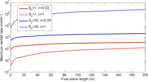
Figure 3.5: Range of rainfall rates for validity of the kinematic wave equation. ...67

Figure 3.6: Schematic representation of the interception model ...73

Figure 3.7: Schematic representation of the model coupling procedure...75

Figure 3.8: Example cumulative root distributions...78

Figure 3.9: Plant water stress function ...79

Figure 3.10: Procedure to determine surface boundary condition ...80

Figure 3.11: Time series of normalised flow response for a range of model domain sizes...83

Figure 3.12: Boundary condition conceptualisation...85

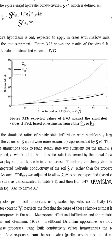
Figure 3.13: expected values of F/G against the simulated values of F/G, based on estimates from either ΩKor ΩK*_...88

Figure 3.14: Example composite hydraulic relationships...92

Figure 3.15: Times series of ensembles from scenario 1 (black lines) and scenario 3 (grey area) ...93

Figure 3.16: Scatter plots of soil structural change parameter values ...94

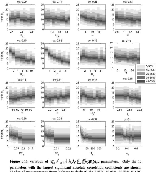
Figure 3.17: variation of qp



p(i)



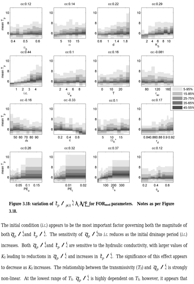
with Θ for FORmod parameters. ...99

Figure 3.18: variation of tp



p(i)



with Θ for FORmod parameters. ... 100

Figure 4.1: General peat classification diagram ... 106

Figure 4.2: Ranges of water retention curves from the literature. ... 112

Figure 4.3: Vegetation Types investigated in Holden (2008)... 114

Figure 5.1: Peatland model domain for (a) intact, (b) drained and (c) blocked drain peatlands... 123

Figure 5.2: Conceptualisation of flow paths in peatlands under different drainage management. . 125

Figure 5.3: Peatland model parameter schematic ... 125

Figure 5.4: Schematic diagram showing saturated subsurface flow over a sloping impermeable bed with the frame of reference (a) rotated, (b) gravitational. ... 129

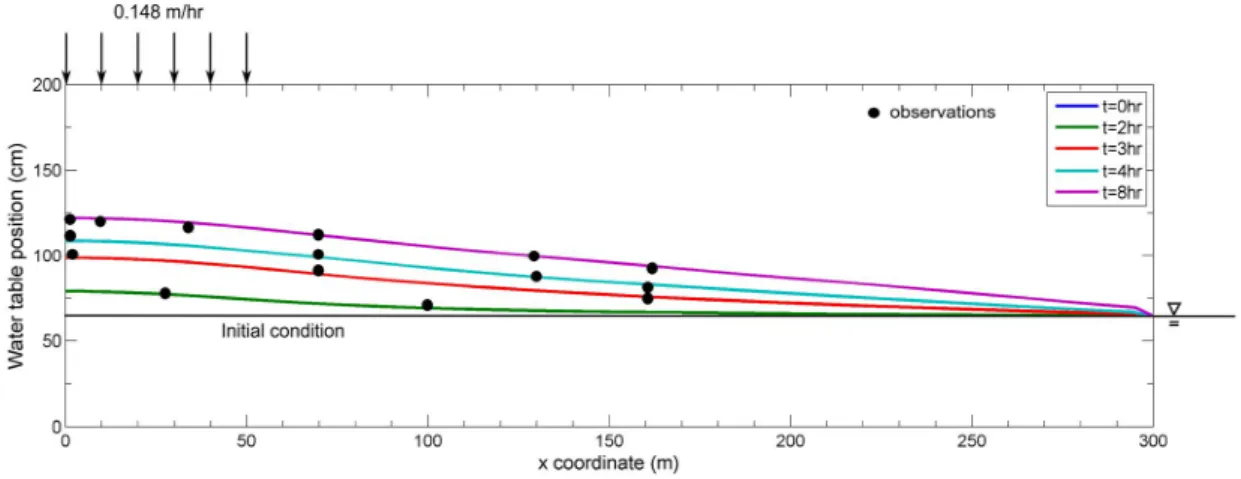
Figure 5.5: Comparison of numerical solution and analytical solution for the Boussinesq equation. ... 130

(14)

Figure 5.7: Comparison of the Holden et al. (2008) friction relationship with flow depth (solid lines)

and a simplified polynomial relationship (dashed)... 137

Figure 5.8: Comparison of friction relationships for a design storm using Holden's (2008) friction relationship (solid lines) and a simplified polynomial relationship (dashed)... 137

Figure 5.9: Comparison of KS(z) representations. KS(dc+da)=0.1 md-1... 139

Figure 5.10: Sample of time series for different KS(z) relationships. ... 140

Figure 5.11: Flow exceedance curve for different Ks(z) representations... 140

Figure 5.12: Sample of time series for different Ep representations... 142

Figure 5.13: Flow exceedance curve for different Ep representations. ... 143

Figure 5.14: Location map of Oughtershaw Beck. ... 145

Figure 5.15: (a) Schematic field site diagram, (b) Model domain and soil blocks. ... 146

Figure 5.16: Cumulative density plots of the a priori and behavioural parameter distributions for each observation point... 148

Figure 5.17: Cumulative density plots of the a priori and behavioural parameter distributions. ... 149

Figure 5.18: Four day sample from the calibration period, showing the largest peak and water table (WT) depth at boreholes A1, A2 and A3... 150

Figure 5.19: Rainfall, flow and upstream water table depth for the verification period. ... 151

Figure 5.20: Poor performance flow hydrograph and water table (WT) depths for boreholes A1, A2 and A3 from verification period. ... 152

Figure 5.21: Good performance flow hydrograph and water table (WT) depths for boreholes A1, A2 and A3 from verification period. ... 152

Figure 5.22: Variation of qp



p(i)



with Θ for the PEATmod parameters. ... 156

Figure 5.23: variation of tp



p(i)



with Θ for the PEATmod parameters... 156

Figure 6.1: River Hodder, Location Map and environment agency flow gauges... 161

Figure 6.2: Footholme flume. ... 162

Figure 6.3: Footholme topography and monitoring. ... 163

Figure 6.4: Footholme soils map (NSRI, 2011)... 164

Figure 6.5: Footholme land surface cover map. ... 165

Figure 6.6: Schematic diagram demonstrating relationships between FORmod parameter sets (Θ).174 Figure 6.7: Photograph of a soil profile exposure of the Belmont soil series within the Footholme catchment... 178

Figure 6.8: Belmont soil characteristics... 179

(15)

Figure 6.10: Peatland drain within the Footholme catchment. ... 183

Figure 6.11: Hydrographs for the largest summer and winter events for the Belmont soil series.. 187

Figure 6.12: Hydrographs for largest summer and winter events for the Wilcocks soil series... 187

Figure 6.13: Increase in peak flow due to LULM change for Belmont soil series... 189

Figure 6.14: Increase in peak flow due to LULM change for Wilcocks soil series... 189

Figure 6.15: Belmont soil series regression estimates of q

 

r versus the corresponding simulated values. ... 193

Figure 6.16: Wilcocks soil series regression estimates of q

 

r versus the corresponding simulated values. ... 194

Figure 6.17: Hydrographs for largest summer and winter events for the Winter Hill soil series. ... 197

Figure 6.18: Increase in peak flow due to drainage management change for Winter Hill soil series (peat). ... 198

Figure 6.19: Regression estimates of the mean change in peak flow (q

 

r ) versus the corresponding simulated values. ... 200

Figure 6.20: q

 

r versus d



q

 

r



following parameter perturbation ... 203

Figure 6.21: Box and whisker plot summarising the distributions of q

 

r caused by various change in LULM scenarios for the soil series present in the Footholme catchment... 207

Figure 7.1: Schematic diagram of metamodel definition... 214

Figure 7.2: Schematic representation of the metamodel structure used in this chapter. ... 217

Figure 7.3: Cumulative density functions (cdfs) of the optimal metamodel parameter sets. ... 221

Figure 7.4: Examples of metamodel hydrographs compared against the original physics based model simulations... 222

Figure 7.5: Increase in peak flow following LULM change for Belmont soil series. ... 226

Figure 7.6: Increase in peak flow following LULM change for Wilcocks soil series... 226

Figure 7.7: Increase in peak flow following LULM change for Winter Hill soil series... 226

Figure 7.8: Comparison of metamodel and physics based model plot scale predictions of q

 

r for the Belmont soil series... 227

Figure 7.9: Comparison of metamodel and physics based model plot scale predictions for the Wilcocks soils series. ... 228

Figure 7.10: Comparison of metamodel and physics based model plot scale predictions for the Winter Hill soil series... 228

Figure 7.11: Comparison of metamodel and physics based model predictions of the mean change in peak flow (q

 

r ) for the Belmont soil series... 229

(16)

Figure 7.13: Comparison of metamodel and physics based model predictions of the mean change in

peak flow (q

 

r ) for the Winter Hill soil series... 230 Figure 7.14: Comparison of improvement in identifiability in metamodel parameters ... 233 Figure 7.15: Physics based and metamodel derived hydrographs at the Footholme flow gauge. ... 237 Figure 7.16: Cumulative density functions (cdfs) of the observed flow prediction performance ... 238 Figure 7.17: Comparison of catchment scale predictions from both physics based models and

metamodel against observations of q

 

r . The red dots are the values for the observed flows. ... 238 Figure 7.18: Schematic land use maps demonstrating the seven different land use scenarios represented in this study... 241 Figure 7.19: Increase in peak flow relative to baseline following LULM change scenario for the Footholme and Bre-sap gauging points. ... 242 Figure 7.20: Comparison of mean peak flow predictions from metamodels and physics based models for all scenarios and all gauges... 243 Figure 7.21: Comparison of mean peak flow predictions from metamodels and physics based models for all scenarios and all gauges... 245 Figure 7.22: Increase in peak flow following LULM change for the Footholme and Bre-sap gauges based on 14 years of simulated flows... 250 Figure 7.23: Plots of estimated return period versus percentage change in peak flows for LULM scenarios at the Footholme and Bre-sap gauges... 252 Figure 7.24: Summary of reductions in peak flows associated with a 10% areal LULM change, derived from simulations in this chapter. ... 257

(17)

List of Tables

Table 2.1: Comparison of ratios of forest to grazed pasture hydraulic conductivity (F/G) for

different soils and tree species...42

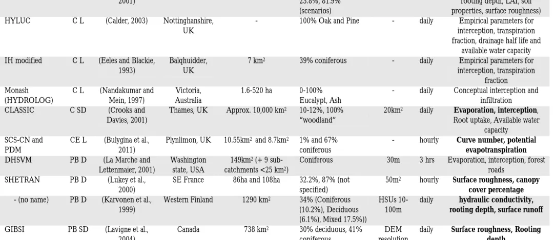
Table 2.2: Summary of models presented in the forest modelling review. ...53

Table 3.1: Summary of model domain size performance ...83

Table 3.2: Boundary condition performance: nRMSE ...85

Table 3.3: Boundary condition performance: q

 

r ...85

Table 3.4: Boundary condition performance simulation time...85

Table 3.5: Summary of scenarios for soil structural representation tests ...91

Table 3.6: Parameter ranges for macroporosity conceptualisation tests...91

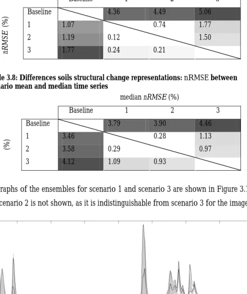
Table 3.7: Differences soils structural change representations: nRMSE between scenario maximum and minimum time series ...93

Table 3.8: Differences soils structural change representations: nRMSE between scenario mean and median time series ...93

Table 3.9: Parameter ranges for generalised sensitivity analysis...97

Table 5.1: Root mean square deviations (mm hr-1_{) between different K}_S_{(z) relationships. ... 140}

Table 5.2: Root mean square deviations (mm hr-1_{) between different E}_p_{representations. ... 143}

Table 5.3: Parameter ranges for Oughtershaw Beck Monte Carlo simulations and general sensitivity analysis... 147

Table 6.1: Footholme flow gauging information... 162

Table 6.2: Footholme climate monitoring information... 162

Table 6.3: Footholme soils HOST classification (Boorman et al., 1995). ... 165

Table 6.4: Slopes angle ranges and soil horizon properties (hydraulic conductivity and thickness) for the mineral soils within the Footholme catchment... 177

Table 6.5: van Genuchten parameter sampling ranges... 179

Table 6.6: LULM specific parameter sampling ranges. ... 182

Table 6.7: Parameter ranges for scenario Monte Carlo simulations... 184

Table 6.8: Median percentage change (decrease) in flow peaks between grazed and other LULM types for the largest summer and winter events. ... 188

Table 6.9: Regression models for values of q

 

r Belmont under different LULMs... 190

Table 6.10: Regression models for values of q

 

r Wilcocks under different LULMs... 191

(18)

m g gc

 

r

d g

q

_



... 193

Table 6.14: Regression models for the Wilcocks soil series to predict



q

_g__m

 

r

,



q

_g__c

 

r

and

 

r

d g

q

_



... 194

Table 6.15: Median percentage change in flows between drained and other drainage management scenarios for the largest summer and winter events. ... 197

Table 6.16: Regression models for intact, drained and blocked values of q

 

r ... 199

Table 6.17 Summary of calculated q

 

r for peatland drainage management change. ... 200

Table 6.18: Regression models to predict the mean change in peak flow (q_d__i

 

r and q_d__b

 

r ). ... 201

Table 6.19: Predicted direction of change of parameter values following drainage management change... 202

Table 7.1: Metamodel internal/state variables and parameter descriptions... 218

Table 7.2: Sampling ranges for the metamodel parameters... 219

Table 7.3: Summary of metamodel prediction performance of plot scale q

 

r . ... 229

Table 7.4: Summary of metamodel prediction performance of q

 

r at the plot scale. ... 231

Table 7.5: Optimised sample range for catchment routing. ... 235

Table 7.6: Comparison of catchment model simulations against observed values of q

 

r , for both predictions based on physics based models and metamodels... 240

Table 7.7: Comparison of catchment model predictions of q

 

r between physics based models and Metamodels. ... 240

Table 7.8: Summary of metamodel prediction performance of catchment scale q

 

r ... 244

Table 7.9: Summary of metamodel prediction performance of q

 

r at the catchment scale... 246

Table 7.10: Minimum, median and maximum reductions in mean catchment peak flow, q

 

r , predicted by both physics based and metamodel predictions for LULM scenarios 2-7... 248

Table 7.11: Minimum, median and maximum % reductions in peak flows for the largest events, Q  , from the 14 year simulation period. ... 254

(19)

Table 7.12: Approximated physics based minimum, median and maximum % reductions in peak

flows for the largest events, Q, from the 14 year simulation period. ... 255 Table 8.1: Summary of predicted median reductions in peak flows associated with LULM change ... 269

(20)

(21)

Chapter 1.

Introduction

1.1.

Background

Recent floods in the UK have focused attention on the effects of rural land use and land management change on flood risk (Wheater, 2006). Since the second World War agricultural intensification has been widespread across the uplands of the UK, with increases in stocking density, ploughing, reseeding and drainage of fields, use of heavy machinery, and the removal of trees from the landscape. Research concerning the effects of land use and land management (LULM) on hydrological processes for lowland arable farming is more readily available than comparable research concerning the uplands, despite their important contribution to runoff caused by high rainfall rates, and generally flashy responses (Marshall et al., 2009). Whether or not these changes in LULM in the uplands are increasing the frequency and magnitude of flooding remains a fundamental scientific question.

LULM changes have been observed to change local surface runoff (e.g. Marshall et al., 2009; O'Connell et al., 2004); however, attempts to isolate such responses at the catchment scale have failed. Several reasons have been proposed as explanations for this failure, including: climate variability, poorly constrained spatial information about the distribution of LULM types and poor historical records of LULM change (Beven et al., 2008). Despite the lack of evidence that effects of LULM changes at the local scale propagate downstream, this does not necessarily mean they do not occur (O'Connell et al., 2007).

1.1.1. The Pontbren experiment and FRMRC

Recognising that there were serious limitations in the existing evidence of the impacts of upland rural LULM change on flooding, in 2004 the Flood Risk Management Research Consortium (FRMRC) (Pender, 2011) funded a major experimental and modelling programme in the Pontbren Catchment in Wales (Wheater et al., 2008). The experiment was run over a seven year period, with monitoring across scales, from plot scale (~100m2_{) to small catchment scale (12km}2_{). The} monitoring programme was developed to provide evidence and quantification of local and small catchment scale impacts of LULM, and to support the development of multi-scale modelling tools.

(22)

At the plot scale (~100m2_{), the effects of land use change on hydrological response were} investigated directly at four sets of manipulation plots, as well as within four tree shelter belts. Data from the hillslope scale (~ 0.1 km2_{) was used to support model development and underpin the} conceptual understanding of the hydrological response of these clay-rich, relatively impermeable, catchments which have been subject to extensive land management intensification and field drainage installation. Catchment-scale (1 to 10 km2_{) monitoring took place at a number of} locations, including different land management regimes, in order to better understand the integrated effects of LULM on flow peaks at different scales of observation.

A number of important lessons were learned from the experimental programme. At the local scale, large reductions in overland flow were observed following tree planting and the exclusion of sheep from previously grazed grassland plots, in as little of one year of tree planting. Smaller, but still significant reductions were also observed from stock exclusion alone. Associated increases in infiltration were observed in the plots, which were strongly correlated to the changes in total runoff volumes. Although these changes were clear, the response for single events and between replicated experimental sites demonstrated high levels of heterogeneity, despite apparent similarity between plots. Results were also confounded by the influence of a strong drought in the pre-treatment period, demonstrating the importance of climate in controlling runoff response, and the potential for non-stationarity in soil properties.

The dominant runoff pathways from the improved grassland hillslope were the drain flow followed by overland flow. The low permeability soils remain saturated for prolonged periods throughout the year, resulting in sustained periods of drain flow (from subsurface tile drains), which dominates the response from the improved grassland hillslope. The drain flow was highly responsive to rainfall inputs, suggesting that macropores or other preferential pathways were directing water to the drains, contributing to the rapid subsurface runoff (Marshall et al., 2009). In larger rainfall events, overland flow also provides a significant contribution to the hillslope runoff. Pore water pressure readings show that overland flow is generated as a result of saturation excess. In only very wet antecedent conditions were overland flow rates observed to exceed drain flow rates. A tree shelterbelt planted across the hillslope was observed to intersect overland flow and consequently reduce downslope surface runoff. However, despite the long and detailed monitoring programme, the fate of the water under the tree shelter belt remained unresolved (Wheater et al., 2008).

The importance of tree shelterbelt siting was explored using a model conditioned to represent the experimental hillslope (see section 1.2.3 for more details about the model). The simulations considered tree shelter belts parallel to the contour at the top or bottom of the field or a shelterbelt

(23)

perpendicular to the contours (Jackson et al., 2008). Even with the only 15% of the area planted, large reductions in overland flow volumes were simulated for the tree scenarios compared to grazed pasture (up to 60%). The most effective configuration for the reduction in overland flow was to have the tree shelterbelt parallel to the contours at the bottom of the field, followed by parallel at the top of the field (Jackson et al., 2008; Wheater, 2006).

Evidence for differences in hydrology related to LULM was also observed in the nested stream flow records. The flow gauges within the catchment each represent subcatchments with different contributing areas and LULM distributions. Differences in stream flow response are observed between subcatchments with significantly different land use management. These impacts were formally identified by McIntyre and Marshall (2010). Significant differences in the response time were identified between the different flow gauges. These differences could be explained by the proportion of the subcatchment area that was under “improved grassland”, the proportion of the subcatchment covered by lakes and ponds, as well as the catchment area. The analysis is not fit for predicting magnitude of responses, but illustrates that such quantification methods are important and that signals of LULM can be observed even at the catchment scale.

The results from the experimental programme were used to support the development of a multiscale modelling methodology, which is outlined in section 1.2.3. The work presented in this thesis represents a component of the second phase of FRMRC, which aims to build upon the evidence and modelling work developed as part of the Pontbren programme to explore impacts of a wider range of LULM questions for other upland sites within the UK.

1.2.

Modelling approach

In their review of the current state of knowledge about the effects of LULM change on flood risk, O’Connell et al. (2004) concluded that new modelling techniques will need to be developed in order to predict the impacts of LULM on flood risk. The key methodological challenge is how to predict catchment scale effects of local scale LULM changes using hydrological models.

Hydrological modelling is an invaluable tool for developing an understanding of the importance of different hydrological processes and ultimately predicting hydrological responses for a range of scenarios. Numerous hydrological models have been developed; however, each model has inherent advantages and disadvantages. To select an appropriate hydrological model structure, it is essential to consider the following factors:

(24)

o What are the key responses of interest i.e. flow (peak flows, low flows), water table levels?

 Supporting data - availability and quality:

o Spatial and temporal observations.

o Measurements of hydrological properties.

o Information from literature.

 Technical requirements:

o Availability of suitable existing models.

o Computational power.

o Modeller expertise.

In this Thesis, the principal modelling objective is to examine changes in high flow responses at the catchment scale related to local scale changes in LULM. It is assumed that ‘supporting data’ will be limited, particularly in terms of identifying historic LULM change and monitoring of small scale processes, as would be the case for most potential applications. In terms of ‘technical requirements’, only standard desktop computers are employed; therefore computational power is limited by current computer processor technology.

Hydrological models can generally be classed as metric, conceptual or physics based models (Wheater et al., 1993). Metric models seek to characterise a system response through statistical relationships developed from observations. Because they are observation based, their suitability for the current LULM change problem is limited, in that the results cannot be safely extrapolated to explore future previously unobserved scenarios; therefore they are not discussed any further.

The structure of conceptual models is defined a priori, based on which processes are perceived to be important. Typically this is done through a series of conceptual stores, for which parameters are calibrated based on observations. The advantage of conceptual models is that they are computationally efficient, but still maintain explicit representations of the main process responses. However, they are not able to represent spatial heterogeneity explicitly, and the model parameters have no physical meaning and must be derived from data (Wheater et al., 1993). If sufficient data are available, it may be possible to map changes in the conceptual model parameters related to LULM, or parameter sets may be restricted based on regionalised response characteristics associated with different LULM types (e.g. Bulygina et al., 2009).

Physics based models use the fundamental equations of physics in order to determine the system response. Although in reality they are simply more complex conceptual models, as they are based

(25)

on fundamental physical equations their parameters could theoretically be measured in the field (i.e. soil thickness, porosity and hydraulic conductivity). However, in reality the scale at which the physical parameters are applied in these models (typically 100s of metres) is not comparable to the scale over which these properties are measured or over which the theoretical bases are developed (Beven, 2001b). Fully distributed physics based models are computationally expensive, and although they are theoretically capable of representing landscape heterogeneity, the associated parameterisation is generally impractical. Although physics based models are helpful in order to assist our understanding of hydrological systems, their computational burden limits their suitability for catchment scale modelling.

1.2.1. Specific challenges for LULM modelling

Numerous attempts have been made to investigate and quantify impacts of LULM change on flooding using a variety of different modelling techniques (for a comprehensive review see O'Connell et al., 2004). At present there is no consensus amongst the hydrological community as to which models are most suitable for traditional hydrological modelling purposes, let alone models that are suitable for predicting the impacts of LULM change.

Reviewing attempts at modelling impacts of LULM change at the catchment scale, O‘Connell et al. (2004, p 109) identified a number of key unresolved issues:

 “There is no generally accepted theoretical basis for the design of a model suitable to predict impacts

 It is not known which data have the most value when predicting impacts

 there are limitations in the methods available for estimating the uncertainty in predictions”

Recognising that there are serious short-comings in most existing rainfall-runoff models for assessing the impacts of LULM change, they recommend that “The modelling should be distributed and be capable of running continuous simulations. It should also be partly or wholly physically based so that the physical properties of local landscapes, soils and vegetation can be represented.” Despite this, they also note that “there are significant methodological issues with extrapolating small scale experimental observations for catchment-scale applications” (O'Connell et al., 2004, p 1)

These recommendations strike on two of the most significant challenges facing hydrologists today. The first is the utility of physics based models; the role and limitations of this class of models has been widely discussed in the literature (e.g. Beven, 1989; Beven, 2001a; Wheater et al., 1993;

(26)

Woolhiser, 1996). The dominance of hydrological processes is generally observed to be scale dependent (Archer, 2003); therefore the second challenge is how to transfer information across scales, both spatial and temporal (Wigmosta and Prasad, 2006). In fact these challenges are not independent; one of the greatest problems for the application of distributed physics based models is one of scale, where compromises in resolution are typically made as the simulation scale becomes larger.

1.2.2. A background to physics based modelling

In order to understand further the specific strengths and weaknesses of physics based models, specifically in light of the key challenges for modelling LULM change highlighted in the previous section, the following section presents a short background of the development and implementation of physics based models in hydrology.

In the late 1960’s Freeze and Harlan (1969) presented a “blue-print” for a physics based distributed hydrological model. They called for a model that coupled together three-dimensional flow of variably unsaturated-saturated flow, two-dimensional overland flow and one-dimensional channel routing. Coupling would be performed through system interdependent boundary conditions, allowing the entire model domain to be represented by one (albeit large) system of equations. Most physics based modelling applications in the literature still use this blueprint; however, computational and data limitations have generally meant that compromises are made in either the resolution (temporal and/or spatial), dimensionality, coupling and/or non-linearity of the process representations (Beven, 2001b).

The first field application of the “blue-print” was by Stephenson and Freeze (1974), for an approximately 270m long hillslope in Idaho, for which runoff is dominated by subsurface stormflow in response to spring snowmelt. Model node spacing was fixed between 1-4 feet, and input data of geology, hillslope geometry, soil hydraulic properties and estimated snowmelt were used. Calibration was through a process of trial and error, based primarily on matching water table measurements at three locations in the hillslope. They found that “no realistic combination of parameter values was found that would provide a suitable calibration unless inflow” from snowmelt was applied in the model in a way that was inconsistent with “the qualitatively observed upslope melting of the snowpack” (Stephenson and Freeze, 1974, p.292). The results were overall not very successful, and the application highlighted a number of challenges that are common to most physics based model applications: (1) simulations were sensitive to initial and boundary conditions, (2) even with complex subsurface data (geology and hydraulic properties), simulations were still poor, (3) computational power limited calibration, validation and sensitivity analysis.

(27)

Numerous physics based models have been developed and applied to various different applications (see Singh and Woolhiser, 2002 for a list of many of the common models), and in most cases have demonstrated some level of predictive success. However, as most applications involve calibration, it is very difficult to assess the validity of the different model structures (Beven, 1993). There has been significant debate about the validity of physics based models, particularly as “the theoretical advantages of physics based models remain unproven in practice” (Beven, 1989 p. 158).

Models are by nature abstractions of reality, and necessarily include approximations and simplifications to represent complex natural phenomena (Woolhiser, 1996). Many of the governing equations used in physics based models are highly non-linear and derived from small scale observations. The applicability of these laws to heterogeneous systems, discretised at a low resolution (10s to 100s of metres) is uncertain; it is thus a leap of faith to assume their validity (Beven, 1989). Many distributed model applications try to avoid this limitation by calibrating the model to replicate observations, thus deriving effective model parameters. The effective model parameters may be different from point scale property measurements and will only be applicable for the specific application minimum scale. Further, effective parameters are generally found to be incapable of replicating the responses of heterogeneous systems, as the non-linear nature of the variably saturated subsurface equations means that the response of a heterogeneous system (particularly with strong surface/subsurface interactions) is controlled by the extremes of the physical properties rather than some sort of average (Binley et al., 1989b). This then reduces the power of speculative simulations using physics based distributed models with parameter values from field based data, as the physical meaning of the parameters diverges from a supposed “reality”, and suitable methodologies to upscale physical parameters a priori are relatively limited (Wigmosta and Prasad, 2006). There are also challenges with representing processes such as macropores, for which Darcy’s law (which relies on the assumption of laminar flow and is the general basis of subsurface flow in the models) may not be applicable (Loague and VanderKwaak, 2004).

The non-linear nature of the variably saturated subsurface equations means that predictions are sensitive to both initial and boundary conditions (Beven, 2001a). Identifying and applying appropriate subsurface boundary conditions for physics based models is very challenging, as they cannot be readily observed and quantified. As such, model performance and calibrated parameters in any physics based hydrological model will be dependent on the assumed definitions of the boundaries (Ebel and Loague, 2006; Stephenson and Freeze, 1974). In order to reduce the dependence of peak predictions on user defined initial conditions, “setting up” periods can be used

(28)

to allow time for the model to equilibrate prior to an event or period of interest (for example, Binley and Beven, 1992, used a 62.5 setting up period of realistic rainfall events)

Physics based models are computationally demanding and highly parameterised. This causes serious problems with calibration, validation, uncertainty quantification and sensitivity analysis. Common calibration techniques, such as Monte Carlo methods or optimisation algorithms are generally not computationally practical. Identifying a single “best parameter set” through manual calibration fails to represent the uncertainty in the predictions and is also subjective when determined through a trial and error process. The large number of model parameters also increases the likelihood that the same model output could be produced by numerous different parameter combinations, the so called problem of “equifinality” (Beven, 1993; Ebel and Loague, 2006). Calibration is often only conducted on single events, and for a sub-set of the potential parameters – those that are perceived to be most sensitive and these simulations can be highly dependent on user defined initial conditions (Beven, 2001a). Although the number of physics based parameters is large, the fact that they are derived from physical relationships already places some constraints on the realistic ranges of the parameter values (Loague and VanderKwaak, 2004). However, simulations conducted “blind” using the distributed physically based model SHETRAN, have shown that even with the restriction that parameter ranges must be physically realistic, that a priori predictions have large uncertainty bounds (Parkin et al., 1996).

While there is a perceived danger of the overselling of the capabilities of physics based models (Beven, 1989; Woolhiser, 1996), there is generally a consensus (even with the strongest critics) that there are some classes of problem, such as the prediction of LULM change, for which physics based models may still be the best approach. With careful acknowledgement of the limitations, restrictions and assumptions used, and realistic estimations of predictive uncertainty, physics based models still have great utility in the prediction of hydrological response (Binley et al., 1991; Loague and VanderKwaak, 2004; O'Connell and Todini, 1996).

1.2.3. Upscaling physics based models to investigate impacts of LULM change

In response to the challenges of applying physics based models described in the previous section, and taking into account the recommendations of O’Connell et al. (2004) for suitable rainfall-runoff models to predict LULM impacts on peak flows, Wheater et al. (2008) recently proposed a potential solution as part of a multi-scale monitoring and modelling programme undertaken in the Pontbren catchment (described earlier in section 1.1.1). The approach aims to combine (1) detailed physics based modelling and (2) conceptual semi-distributed catchment modelling, with the objective of propagating local scale effects of LULM change to the catchment scale (Wheater et al., 2008). This

(29)

approach incorporates an understanding of how physical properties change at the local scale into a more flexible and computationally efficient catchment scale conceptual model.

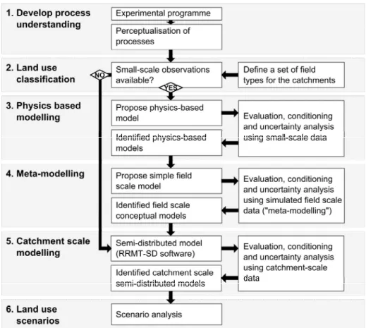
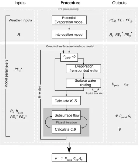
The first step is the discretisation of the catchment into a number of runoff generating elements. In the Pontbren catchment, the catchment was subdivided into field units of non-uniform sizes (which are assumed to be hydrologically independent). This discretisation was largely driven by the dominance of surface and near-surface runoff and the extensive use of edge-of-field ditches within the catchment. Each of the fields was classified by its soil type and LULM. Each combination of soil and LULM is referred to as a runoff class. Physics based models, conditioned on detailed monitoring data, were developed to represent each of the runoff classes present within the Pontbren catchment. These models were then used to condition simpler “metamodels” (conceptual models that are inherently linked to the physics based models). The metamodels were then used in a semi-distributed catchment model (Jackson et al., 2008); local runoff from each runoff generating element is approximated based on the runoff predicted by the metamodel corresponding to the field runoff class. Local runoff from the fields is then aggregated using a simple stream routing algorithm to give estimates of streamflow at the catchment outlet. In this way, local scale information is “upscaled” in a computationally efficient way, allowing sub-grid variability due to differences in LULM to be accounted for in the semi-distributed model runoff generating elements. A schematic representation of the procedure is show in Figure 1.1.

(30)

Figure 1.1: FRMRC 1 modelling approach

Using this modelling approach, catchment scale effects of local LULM interventions were quantified for the Pontbren catchment. Reductions in peak flows were observed for LULM scenarios with planting of tree shelterbelts, and increases in peak flows were observed for grazing intensification scenarios (Wheater et al., 2008). Despite the previously mentioned limitations and challenges associated with the implementation of physics based models to real complex systems, the Darcy-Richards based physics based model employed to replicate the Pontbren hillslope response showed a good performance in simultaneously predicting drain and overland flow (Jackson et al., 2008; Wheater et al., 2008). This was in spite of the major simplifications of the model, which included: (1) a homogeneous, isotropic, stationary soil, with hydraulic conductivity fixed based on field measurements, (2) no representation of complex hillslope topography, (3) no explicit representation of macropores and (4) no hysteresis in soil properties. Although good performance was noted for drain flow and overland flow predictions, poorer performance was achieved in replicating observed tensiometer records, in particular dry periods, which could be as a result of some of the process simplifications (Jackson et al., 2008). It is also noted that the experimental hillslope had relatively simple topography; hence a more complex topographic was unnecessary for this particular example.

(31)

The modelling approach demonstrated at Pontbren was considered to be successful, as the impacts of the LULM interventions were identifiable, in that the effects of LULM change could be discriminated from model and parameter uncertainty. However, this tool was developed and applied to a data-rich environment, supported by an extensive field programme; in most applications this amount of supporting data will not be available. Therefore, if this modelling approach is to be considered as a generic tool to provide strategic policy guidance, it is necessary to consider the role of physics based models and the new modelling approach in a data-scarce environment.

The lack of small scale data for a catchment causes problems for the modelling approach outlined in Figure 1.1, given the need for data to condition the physics based models. However, even in the absence of such data, physics based models may still be an effective way to upscale local changes to the catchment scale, as our understanding of the impacts of LULM changes is largely restricted to changes in small scale processes (i.e. interception and infiltration) and physical properties (i.e. hydraulic conductivity and water retention curves).

Even without hydrological measurements for a site of interest, physics based models can be developed and tested using a combination of (1) information about small scale hydrological processes and properties from the literature, (2) information from surrogate sites, and (3) qualitative information about hydrological responses through engagement with field hydrologists. By using such data to parameterise the physics based models, uncertainty in a priori parameters is likely to increase. Limited data also implies that there is a greater chance that the model structures will be poorly defined (Ebel and Loague, 2006), thereby adding additional uncertainty to the model predictions (Butts et al., 2004). The extent to which uncertainty can be constrained by such data is not clear and remains a key question for future research. It is also noted that physics based models may improve understanding of runoff processes and the dominant physical controls by providing a mechanism to test the suitability of perceptualisations against observations of real world behaviour (either qualitatively or quantitatively). Such qualitative insights may be of value when: (1) considering the effects of LULM change and (2) designing effective monitoring programmes that supply supporting data that reduce model uncertainty.

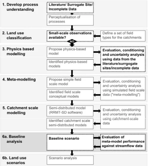
An alternative modelling approach that takes data scarcity into account is proposed and is shown in Figure 1.2. The differences in modelling approach between Figure 1.1 and Figure 1.2 are shown in bold text and dashed boxes in Figure 1.2. The primary change is that data scarcity no longer automatically leads to a bypass of the physics based modelling (stage 3.).

(32)

Figure 1.2: Data scarce modelling approach

1.3.

Working assumptions

In order to evaluate the suitability of the upscaling procedure to data scarce environments, a number of working assumptions need to be established as a starting point for the research. As far as possible, the procedure employed at the Pontbren catchment is used, with the adaptations for data scarce catchments shown in Figure 1.2.

In addition, it is assumed that the catchment discretisation into runoff generating elements can be performed using a uniform grid, rather than the irregular cell units used in the Pontbren catchment. A uniform grid was deemed to be more achievable for a catchment for which there is little detailed information, and particularly when field drainage networks are not present or not explicitly identified. In the catchment application presented in this Thesis, a 200m x 200m grid is applied. This scale was chosen to balance the desire to represent localised LULM interventions without restrictively increasing the computational burden of the semi-distributed catchment model.

(33)

With this grid discretisation assumption, it then follows that the physics based models for each runoff class should represent 200m x 200m hillslopes. The models need to be representative of all runoff class grid cells, and as such will be modelled as idealised uniformly sloping hillslopes.

Other significant assumptions made in the Pontbren application that are used as working assumptions in this research include:

1) Runoff generating elements are independent. Although this assumption has some physical grounding in the case of the Pontbren application, where fields (runoff generating

elements) are isolated from each other, the validity for a uniform grid discretisation is less clear.

2) Simplified routing is sufficient to aggregate locally generated runoff in order to make catchment scale predictions.

These working assumptions are not explicitly examined as part of this Thesis, however, they are considered in the final evaluation of the procedure performance (Chapter 8).

1.4.

Aims and Objectives

In this Thesis the procedure shown in Figure 1.2, with the working assumptions listed in section 1.3, is applied to a test catchment with scarce supporting data – the Footholme catchment (introduced in more detail in Chapter 6). The modelling application is used to assess whether identifiable impacts of LULM change at the local and catchment scales can be predicted using physics based models and their upscaled responses, despite data scarcity.

Specific objectives include:

1) Predict the effects of LULM change at multiple scales and evaluate whether these changes can be discriminated from effects of model and parameter uncertainty.

2) Assess the value of speculative simulation given data scarcity, and determine whether any further value can be gained by using information from surrogate sites.

3) Identify the principal processes and properties associated with LULM change that most greatly influence changes in peak flows, and assess their scale dependency.

4) Identify monitoring strategies to produce data that would most greatly improve the structure and predictive power of the local scale physics based models.

(34)

5) Propagate uncertainty through the upscaling procedure in order to identify the stages of the methodology that, if improved, would most greatly assist in the reduction of catchment scale prediction uncertainty.

1.5.

Thesis outline

To achieve the Thesis objectives, a case study site was selected on which to apply the methodology outlined in Figure 1.2. The Footholme catchment is a 25km2_{sub-catchment of the Hodder River.} The Footholme catchment was selected as it is currently undergoing widespread LULM change, particularly in regard to: (1) forestry management (forests are located on the mineral soils), making changes to both coniferous plantation as well as strategic planting of deciduous trees and (2) drainage management of the upper extents of the catchment that are predominantly covered in blanket peatland. Importantly, the LULM and soil type combinations present in the Footholme catchment are different from those at the Pontbren catchment, so direct application of the metamodels developed for Pontbren is not appropriate. The two different LULM categories (forestry and peatland drainage management) present two different sets of modelling challenges, in terms of the representation of change as well as availability of information from surrogate sites and literature on which to develop and test the physics based models.

Forestry LULM scenarios are implemented exclusively through model parameter changes, such as changes in evaporation, interception and soil structural properties. There is a significant pool of knowledge to draw from in the literature regarding the processes and properties related to forests and their hydrological function. However, supporting knowledge to develop and condition the local scale physics based model is limited to information from literature, as data from an appropriate surrogate site was not available for this study.

Peatland drainage is implemented through an open ditch drainage network. Drainage management scenarios considered in this Thesis are: intact, drained and blocked drains. Because of the nature of the land management, the different drainage management scenarios must be represented primarily through model structural changes. Knowledge of processes, properties and peak flow responses associated with peatland drainage management is relatively limited, particularly in contrast to the large amount of information available about forestry LULM. However, data from a surrogate drained peatland site is available to assist in the evaluation and conditioning of the local scale physics based model.

(35)

The development and testing of the physics based models to represent forestry and peatland drainage management scenarios are presented in chapters 2-5. Chapter 2 is a review of hydrological processes and responses associated with forestry, leading to the development of a conceptual model. In chapter 3 the conceptual model is developed into a forest hillslope mathematical model (FORmod). The numerical solution procedures are presented along with an analysis of the sensitivity to the conceptualisation of some of the key hydrological controls. Components of the model structure are compared against analytical solutions. Finally a general parameter sensitivity analysis is conducted.

In Chapter 4, a review of peatland hydrology is presented, focusing on the primary controls on peak flow response. Based on the conceptual understanding of peatland hydrological functioning developed in Chapter 4, a plot scale physics based hydrological model (PEATmod) is developed in Chapter 5. The model has the capability to represent intact, drained and blocked drain peatlands. Components of the model structure are compared against analytical solutions, and the complete coupled model is then tested and parameter uncertainty estimated using a dataset for a surrogate drained peatland site in the Yorkshire Dales, UK. Finally, a broad sensitivity analysis is conducted on the model in order to assess the general agreement of the model with responses quoted in the literature, and to identify those processes and properties to which the peak flow response is most sensitive.

Chapter 6 describes the Footholme catchment, and both physics based models (FORmod and PEATmod) are used to simulate potential local scale runoff responses for combinations of soil type and LULM specific to the test catchment. The sensitivity of the peak flow runoff response to the model parameters is assessed, and the identifiability of the local scale changes in runoff response related to LULM change is evaluated.

The local scale runoff response developed in Chapter 6 is then used in Chapter 7 to train metamodels. The identification of multiple optimum parameter sets (for each local response time series) for a selected metamodel structure is presented. The uncertainty introduced due to the metamodelling procedure is quantified, both for the entire time series, as well as just for the largest peak flows and their differences between LULM types. The catchment scale semi-distributed model structure is introduced and the model routing parameters are restricted based model performance against the flow observations. Additional uncertainty introduced by the metamodels at the catchment scale is evaluated by comparing simulations from the catchment scale semi-distributed model, for a range of LULM scenarios, with local runoff generation predictions directly from the physics based model outputs against predictions made using the metamodels. Longer

(36)

term simulations (14 years) are performed for a selection of possible LULM scenarios for the catchment, using the semi-distributed catchment model with local runoff predicted by the metamodels. The identifiability of the predicted effects of LULM change is evaluated taking into account the accumulated model assumptions and uncertainties.

Finally, Chapter 8 presents an evaluation of the modelling procedure and addresses the previously defined objectives, describes contributions of this work and makes suggestions for areas of future research.

(37)

Chapter 2.

Forest hydrology literature review

Forests cover approximately 30% of the earth’s land area (FAO, 2001); therefore the relationship between forests and water has the potential to have major impacts on global hydrologic cycles. Forests can regulate flows and reduce sediment production, but they also provide a number of other important services, including: habitats, wood products (such as building materials and paper), recreation and energy production. They can be natural, semi-natural, or managed plantations. The trees that constitute forests are commonly split between: softwoods/hardwoods, coniferous/broadleaved, evergreen/deciduous. For common UK species, softwood, coniferous and evergreen are synonymous, and hardwood, broadleaved and deciduous are synonymous, although globally across all species there are some exceptions.

Both water and forests are important natural resources and they are related through a large number of complex feedback mechanisms. The objective of this review is to examine these relationships, and in particular focus on those processes that may be significant in relation to flooding, in order to allow well-informed development and evaluation of a forest physics based model. Hydrological responses from the catchment scale down to the field scale will be examined, as well as properties of forests and forest soils. Methods used to model forest hydrology are compared examining differences in model structures, scales and applications. Finally a summary of the key findings of the review is presented.

2.1.

Impacts of forestry on catchment scale hydrological response

One of the earliest studies in the UK of forest hydrology was conducted during the 1950s by Law (1957a; 1957b) in the Hodder Catchment (NW England). The study examined the annual water yields of two small catchments, one forested and the other pasture. Water yields were found to be significantly lower from the afforested area in comparison to surrounding grassland. The results were controversial, as forests had (misguidedly) been generally thought to increase water yields, and as such it had been government policy to afforest catchments that fed reservoirs (McCulloch and Robinson, 1993). These results raised awareness about the lack of understanding of the impacts of forests on hydrology and led to the development of a number of experimental sites in the UK uplands to investigate the impacts of forests on the water balance, and more generally on the

(38)

hydrological and water quality regimes of upland catchments. These include the paired catchment studies at Plynlimon Wales) (Hudson et al., 1997a; Kirby et al., 1991), Llanbrynmair (mid-Wales)(Hudson et al., 1997b) and Balquhidder (central Scotland) (Johnson and Whitehead, 1993), and the single catchment study at Coalburn (NW England) (Robinson, 1986; Robinson, 1990).

The Plynlimon catchment study began in the 1960s and is still ongoing today. It is a paired catchment study in upland Wales, in the headwaters of the Severn (8.7km2_{, 70% forest) and the} Wye (10km2_{, 100% grassland). The original intent for the study was to build upon Law’s work and} examine the impacts of coniferous forestry on water yields. Analysis of long term timeseries data led to results similar to those observed by Law. Greater evaporation was observed from coniferous forests (29-32% of rainfall) in comparison to grassland (15-17% of rainfall), and most of this evaporation was from water intercepted by the trees (Kirby et al., 1991).

The Balqhuidder paired catchments are located in the highlands of Scotland. The catchments receive high rainfall, snowfall and winds and generally have low temperatures. The soils are largely thick peat deposits overlying glacial till (Johnson and Whitehead, 1993). Two catchments were selected (each approximately 7km2_{), one which contained significant areas of coniferous forest} (34.4%), and the other was moorland. After a baseline period, much of the forested catchment was felled, and tree planting began in the moorland catchment. The experiment is not typical of paired catchment studies, where usually one catchment is left as a baseline and the other manipulated; this may have been why the impacts of the LULM changes were generally not found to be detectable in the daily flow record (Calder, 1993; Jakeman et al., 1993). However, the impacts of the baseline forestry were visible in the catchment water balance, with differences in total evaporation greater by 30% in the forested catchment (Hall and Harding, 1993), which is in agreement with the observations at Plynlimon.

While the evidence for decreased annual water yield associated with forests is strong at both Plynlimon, Balquhidder and other sites around the world (Bosch and Hewlett, 1982), impacts of forests on r