T A R T U
U N I V E R S I T Y
FACULTY OF MATHEMATICS AND COMPUTER SCIENCE
Institute of Mathematical Statistics
Frazier Carsten
Overdispersed Models for Claim
Count Distribution
Master’s Thesis
Supervisor: Meelis K¨
a¨
arik, Ph.D
Contents
1 Introduction 3
2 Classical Collective Risk Model 4
2.1 Properties . . . 4 2.2 Compound Poisson Model . . . 8
3 Compound Poisson Model with Different Insurance Periods 11
4 Overdispersed Models 14
4.1 Introduction . . . 14 4.2 Causes of Overdispersion . . . 15 4.3 Overdispersion in the Natural Exponential Family . . . 17
5 Handling Overdispersion in a More General Framework 22
5.1 Mixed Poisson Model . . . 23 5.2 Negative Binomial Model . . . 24
6 Practical Applications of the Overdispersed Poisson Model 28
Kokkuv˜ote (eesti keeles) 38
References 40
Appendices 41
A Proofs 41
1
Introduction
Constructing models to predict future loss events is a fundamental duty of actu-aries. However, large amounts of information are needed to derive such a model. When considering many similar data points (e.g., similar insurance policies or in-dividual claims), it is reasonable to create a collective risk model, which deals with all of these policies/claims together, rather than treating each one separately. By forming a collective risk model, it is possible to assess the expected activity of each individual policy. This information can then be used to calculate premiums (see, e.g., Gray & Pitts, 2012).
There are several classical models that are commonly used to model the number of claims in a given time period. This thesis is primarily concerned with the Poisson model, but will also consider the Negative Binomial model and, to a lesser extent, the Binomial model. We will derive properties for each of these models, both in the case when all insurance policies cover the same time period, and when they cover different time periods.
The primary focus of this thesis is overdispersion, which occurs when the observed variance of the data in a model is greater than would be expected, given the model parameters. We consider several possible treatments for overdispersion, particularly those that apply to the Poisson model. First, we attempt to generalize the Poisson model by adding an overdispersion parameter (see, e.g., K¨a¨arik & Kaasik, 2012). Next, we search for ways to convert an overdispersed Poisson model to a Negative Binomial model. We will derive some basic properties (such as expectation, variance, and additivity properties) for all of the models mentioned above.
Finally, results of this thesis are explored in a practical sense, by attempting to fit computer-generated data into an overdispersed Poisson framework.
2
Classical Collective Risk Model
2.1
Properties
The Classical Collective Risk Model is a method of modeling insurance claims using grouped claims. In other words, a group of similar claims are all clustered together, rather than each being considered separately. This can be very useful when dealing with large amounts of similar data, such as claim sizes for car crashes or property damage.
Consider an insurance portfolio composed of some number of insurance policies, with each policy having a given distribution of loss sizes. Let N be the number of claims for this portfolio in a given time period (for example, one year). Let
Zj be the individual claim amounts, j = 1,2, ..., N. For the moment, assume
that individual claims are independent from one another, and that they are also independent ofN. (Later, we will see what can happen when certain independence requirements are violated.) Then, the total claim amountSof the portfolio is (see, e.g., Gray & Pitts, 2012):
S =
N
X
j=1 Zj
In general, the procedure for premium calculation using the collective risk model is as follows:
1. Group the policies of the portfolio into homogenous groups, or subportfo-lios. A subportfolio is homogenous when all of its policies have independent, identically distributed (i.i.d.) risk severities and frequencies.
2. Estimate the frequency (number of claims) and severity (average claim size) for each subportfolio.
3. For each subportfolio, estimate the total claim amount using the collective risk model. Proportionally divide the total expected claim amount between policies in the subportfolio.
portfolio into subportfolios) is outside of the scope of this thesis, so we will not discuss it. For our purposes, we need only to assume that a suitable algorithm exists, and that the portfolio is clustered accordingly.
For any given subportfolio, let S∗ be the total claim amount and N∗ the total
number of claims. Let n be the number of policies in the subportfolio, and let Ni
and Yi, respectively, be the frequency (number of claims) and total claim amount
for the ith policy (i = 1, ..., n). Let Zij be the jth claim from the ith policy
(j = 1, ..., Ni). If certain indices are irrelevant to the current discussion, they may
be omitted: N, Y may be written instead of Ni, Yi, respectively, and Zi or Z
instead of Zij. If all of the above is assumed, then just like the portfolio as a
whole, S∗ = PN∗
j=1Zj. Furthermore,
ES =EN∗·EZ, (1)
V arS =EN∗·V arZ+ (EZ)2·V arN∗. (2)
Where EX and V arX are, respectively, the expected value and variance of X. These properties of the collective risk model are well-known, but their proof is included in Appendix A.
These computations also hold for the individual policy level, so we see that:
EYi =ENiEZ, (3)
V arYi =ENiV arZ+ (EZ)2V arNi. (4)
Furthermore, we wish to find relations between the expectations and variances of
N∗ and N. We see that N∗ =
n P i=1 Ni, so: EN∗ =E n X i=1 Ni ! = n X i=1 E(Ni) = n X i=1 EN =n·EN.
Since all Ni are independent and identically distributed, we see that: V arN∗ =V ar n X i=1 Ni ! = n X i=1 V ar(Ni) = n·V arN.
If we assume that a portfolio can be divided into homogenous subportfolios, and that the total claim amount can be estimated for each subportfolio, then the pure premium for any given policy is the total pure premium of the subportfolio divided by the number of policies.
Note: We have been acting on the assumption that all of the policies have the same time duration. This is quite unlikely, so later in this paper, we will need to find a way to consider policies of different durations.
It is necessary to choose a distribution of claim frequency. The three classical distributions, which are the most commonly used and quoted, are the Poisson, Binomial, and Negative Binomial distributions (see K¨a¨arik & Kaasik, 2012). Consider a random variable N.
• N follows the Poisson distribution (N ∼P o(λ)) if its probability mass func-tion is given as:
f(k) = P(N =k) = λ
k
k!e
−λ,
Where λ >0 is a given parameter (also called theintensity), and k is some nonnegative integer. Then, f(k) gives the probability of k events occurring (in a specified time period depending on the model). For the Poisson distri-bution, EN =V arN =λ, so the Poisson distribution works well when the mean and variance are approximately equal.
Intuitively, we may interpret the Poisson distribution as giving the proba-bility thatk independent, identically distributed, randomly-occurring events will take place in one unit of time, given that the expected (average) rate
to see why the Poisson distribution is so commonly used for insurance: it is a very simple way of forecasting random, independent loss events (car acci-dents, property damage, etc.), if the average rate of these events is known beforehand.
• N follows the Binomial distribution (N ∼Bin(n, p)) if its probability mass function is given as:
f(k) = P(N =k) = n k pk(1−p)n−k,
wheren∈N andp∈[0,1] is a given probability. Note that for this
distribu-tion, k can only take values from 0 to n, all other values have probability 0. For the Binomial distribution. EN =np, V arN =np(1−p). Sincep∈[0,1], clearly EN > V arN.
Intuitively, the Binomial distribution models a process with only two possible outcomes being run multiple times. If the probability of success is p, then the Binomial distribution gives the probability of k successes out of a total ofntrials. The simplest instance of a Binomial distribution involves flipping a coin n times, and counting the number of times that heads occur.
For insurance, the Binomial distribution can be useful for modeling the num-ber of claims: if a portfolio has n i.i.d. policies, and each policy can incur at most one loss event with probability p, then clearly the number of claims will have a Binomial distribution.
• N follows the Negative Binomial distribution (N ∼ N B(r, p)) if its proba-bility mass function is given as:
f(k) = P(N =k) = k+r−1 k (1−p)rpk,
wherer∈N andp∈[0,1] is a given probability, as before. For the Negative
Binomial distribution,EN = 1pr−p, V arN = (1−prp)2. Therefore, EN < V arN.
inter-preted as modeling a process with only two outcomes that is run multiple times. If the probability of failure is 1−p, and the process is repeated until
rfailures occur (and then stopped), then the Negative Binomial distribution gives the probability that k successes occur before the process is halted. A very simple example of the Negative Binomial distribution involves flipping a coin until it comes up tails a total of rtimes, and then counting the number of times that the coin displayed heads.
For most cases in insurance, EN ≤ V arN, so the Binomial distribution is not often used. In general, we prefer to employ the Poisson distribution, due to its ease of use and wide range of applicability; however, it tends to fail when the mean and variance are notably different.
When a model has a variance that is greater than we would expect from the distribution that we use to describe it, we say that the model is overdispersed, or that it has overdispersion. For the Poisson model, clearly, overdispersion occurs when V arN > EN. Note that overdispersion does not necessarily mean that the entire model must be discarded; however, the distribution must be modified in some way. We will discuss overdispersion and possible treatments later in this paper; for now, it will not be considered.
2.2
Compound Poisson Model
Thus far we have begun to discuss ways of modeling the number of claims, but not the distribution of claim sizes. Let N ∼ P o(λ); that is, the random variable N has a Poisson distribution with parameter λ. Furthermore, let Z1, Z2, . . . be
i.i.d. random variables with a given distribution, that are also independent of N. Consider S = PN
i=1
Zi, the sum of a ”Poisson-distributed number” of i.i.d. random
variables. Then, S is said to have a Compound Poisson distribution.
At this point, it is useful for us to move from a fixed time model to one that can be used for varying periods of time. This is, in fact, quite simple to achieve with a Poisson model. We know that EN = λ, so λ can be considered as the
week). N is homogenous; that is, λ does not change over time. Because of this, we may consider the process N(t), defined as the number of events occurring in timet, when the number of events occurring in each unit of time is an independent realization of N. N(t) is then called a counting process with intensity λ (since
EN(1) =EN =λ).
The Compound Poisson Model is extremely useful for the classical collective risk model, because it allows us to describe the number of claims in timet asN(t), the individual claim sizesZi, and the total claim size S for a given portfolio.
Let S(t) be a compound Poisson process. Let N(t) and Zi be as defined above,
i= 1, . . . , n. Then, S(t) = N(t) X i=1 Zi.
We want to derive some of the general properties of this model, starting with the mean and variance. However, to do this, we first need to demonstrate the additivity property of the Poisson distribution.
Proposition 2.1. If N1, . . . , Nn are independent Poisson random variables with
parameters λ1, . . . , λn, respectively, then their sumN =N1+· · ·+Nn is a Poisson
random variable with parameter λ=λ1+· · ·+λn.
This property is well-known, but its proof is included in Appendix A.
We will return to this additivity property several times during this paper. However, it is particularly useful for our current discussion of the counting process N(t). First, we assume that t is a positive integer. (This is a reasonable assumption for our purposes, since we generally do not want to consider periods of time smaller than one day.) IfN1, . . . , Ntare i.i.d. and each identically equal toN, thenN(t) =
N1+· · ·+Nt is still a Poisson process, with parameterλ1+· · ·+λt=tλ.
Let EZ = µ. We are finally prepared to derive the expectation and variance of
S(t).
As we showed in equation (1), the expected value ofS(t) is:
Furthermore, from equation (2), the variance of S(t) is:
V ar(S(t)) =EN ·V arZ+ (EZ)2·V arN =tλ·V arZ+EZ2tλ
=tλ(V arZ+ (EZ)2) = tλ·E(Z2).
V ar(S(t)) = tλE(Z2) (6) The Compound Poisson process is largely useful because it allows us to consider the total claim amount rather than looking at each claim separately, which is cum-bersome when dealing with a large number of claims. Of course, the model requires all of the usual restrictions placed on the Classical Collective Risk Model.
The additivity property of the Poisson distribution also carries over to the Com-pound Poisson process: Let S1(t), . . . , Sn(t) be independent Compound Poisson
processes with intensities λ1, . . . , λn. Then S(t) = S1(t) +· · ·+Sn(t) is a
Com-pound Poisson process with intensityλ =λ1+· · ·+λn.
Once again, we will use a proof by induction. For n = 1, the solution is trivial. Forn = 2, S(t) =S1(t) +S2(t) = NX1(t) i=1 Zi+ NX2(t) j=1 Zj = N1(tX)+N2(t) k=1 Zk = N(t) X k=1 Zk.
As we have proven, N(t) is a Poisson counting process with intensity λ=λ1+λ2, so S(t) is a compound Poisson process. The remainder of the inductive proof is straightforward and directly follows the proof of the additivity property for Poisson random variables.
The additive property helps us to simplify our model still further, by allowing us to group together Compound Poisson-modeled subportfolios that have the same claim size distribution.
3
Compound Poisson Model with Different
In-surance Periods
It is highly unlikely that all of the insurance policies in a portfolio will have the same time duration. Therefore, we need to extend the model to take different time periods into account.
For a given portfolio, we define ni as the number of claims in the ith policy, ti
as the corresponding insurance period (i.e., the length of time of the policy), and
nij as the number of claims of policy i in time unit j (e.g., one day or one year).
Then, we can say that ni = ti
P
j=1 nij.
Assume that we are considering a homogenous subportfolio. Then, we can say that the claim numbers (per unit time) nij are independent instances of the random
variable Nij for all i = 1, . . . , n and j = 1, . . . , ti. (We may also write N[i] if the
exact time j is irrelevant). Therefore, each ni is an independent instance of the
random variable Ni = ti
P
j=1
Nij. As we know, Ni is Poisson distributed if all Nij are
also Poisson distributed. We consider equations (4) and (5), and apply them to this model, to get estimates for the mean and variance of the claim amount for risk i, i = 1, . . . , n. Observe that ENi = tiEN[i], and since ENi = V arNi and
EN[i]=V arN[i], thenV arNi =tiV arN[i]=tiV arNij. Therefore,
EYi =tiEN[i]EZ, (7)
V arYi =tiEN[i]V arZ+ti(EZ)2V arN[i]. (8)
Consider howNi is distributed ifNijhas a Poisson, Binomial, or Negative Binomial
distribution.
• IfNij ∼P o(λ): In section 2.2, we proved that the sum ofn Poisson random
variables with parameters λ1, . . . , λn is a Poisson random variable with
pa-rameterλ=λ1+· · ·+λn. Thus, sinceNi = ti
P
j=1
Nij, we see thatNi ∼P o(tiλ).
Y ∼Bin(m, p). We will show that X+Y ∼Bin(m+n, p). Using a convolution argument, we see that:
P(X+Y =z) = z X k=0 P(X =k)P(Y =z−k) = z X k=0 n k pk(1−p)n−k m z−k pz−k(1−p)m−z+k =pz(1−p)m+n−z z X k=0 n k m z−k
Vandermonde’s Identity (Quaintance, 2010) tells us that this sum equals
m+n z
, so:
P(X+Y =z) = m+znpz(1−p)m+n−z.
Thus, X+Y ∼Bin(m+n, p). A simple inductive argument will then show that, for n Binomial random variables Xi ∼ Bin(mi, p), i = 1, . . . , n, their
sum X1+· · ·+Xn ∼Bin(m1+· · ·+mn, p).
Therefore, ifNij follows a Binomial distribution, Ni ∼Bin(tin, p).
• If Nij ∼ N Bin(r, p): Similar to the Binomial distribution, the sum of
N Bin(r1, p), . . . , N Bin(rm, p) is N Bin(r1 +· · ·+ rm, p). Once again, we
will prove this using a convolution argument. Consider X ∼ N B(r, p),
Y ∼N B(s, p). Then, P(X+Y =z) = z X k=0 P(X =k)P(Y =z−k) = z X k=0 k+r−1 k (1−p)rpk z−k+s−1 z−k (1−p)spz−k = (1−p)r+spz z X k=0 k+r−1 k z−k+s−1 z−k .
There is a combinatoric identity (Quaintance, 2010) stating that: z X k=0 a+k k b+z−k z−k = a+b+z+ 1 z
If we set a=r−1,b =s−1, then we see that: P(X+Y =z) = (1−p)r+spz z+r+s−1
z
, so X+Y ∼N B(r+s, p).
Therefore, ifNij follows a Negative Binomial distribution,Ni ∼N Bin(tir, p).
Next, we will assume that for a given portfolio (or subportfolio), the frequency per time unit, Nij, is Poisson distributed: Nij ∼ P o(λ). Then during the insurance
period for the ith policy, Ni ∼ P o(tiλ), where ti is the length of the insurance
period. In order to find the score function for λ, we first need the log-likelihood function.
Fori= 1, . . . , n, letnibe independent realizations of Poisson distributionsNi with
corresponding parameters λti. Then, the likelihood function for the Compound
Poisson distribution is:
L(λt1,· · · , λtn|n1,· · · , nn) = n Y i=1 P(ni|λti) = n Y i=1 (λti)nie−λti ni! .
Then, the corresponding log-likelihood function is: lnL(λt1,· · ·, λtn|n1,· · · , nn) = n X i=1 ln (λti)nie−λti ni! = n X i=1 (ni(ln(ti) + ln(λ))−λti−ln(ni!)).
The score function is the partial derivative of the log-likelihood function with respect to the parameter:
s(λ) = ∂ ∂λ n X i=1 (ni(ln(ti) + ln(λ))−λti−ln(ni!)) = n X i=1 (ni λ −ti) = 1 λ n X i=1 ni− n X i=1 ti
By setting s(λ) = 0 and solving for λ, we obtain the maximal value estimate for
λ: ˆ λ= n P i=1 ni n P i=1 ti . (9)
4
Overdispersed Models
4.1
Introduction
As we discussed earlier in section 2.1, the Poisson model requires that the mean and variance are equal. While this requirement is reasonable from a theoretical standpoint, it is highly restrictive in a practical sense; in general, the mean and variance of a distribution are not dependent on one another. However, a Poisson distribution is still highly desirable because of its ease of use and extendability characteristics, so we would like to find a way to apply the Poisson model when this restriction does not hold.
As we said before, if the variance of a model is greater than we expect, then it is overdispersed, or has overdispersion. In the case of the Poisson model, overdisper-sion occurs when V arN > EN.
Note: If the model has smaller variance than we expect, we say that it is underdis-persed. Underdispersion is more unusual than overdispersion, and it is also much
less problematic for our purposes: data points that are clustered tightly together are easier to deal with than data points that are very spread out. Because of this, we will not discuss underdispersion.
Let us define the parameterϕ, called the overdispersion parameter. For the Poisson distribution,ϕ is defined byV arN =ϕEN; or alternatively,ϕ = V arNEN . Note that, for the purposes of insurance, it is reasonable to assume that EN ≥ 0. So if we assume that V arN > EN as well, then clearly ϕ > 1. In this way, we can use a model similar to the classical Poisson model, but we estimate parameters using a quasi-likelihood framework. The quasi-likelihood function is similar to a log-likelihood function; however, the quasi-log-likelihood function is not based on any specific probability distribution. Other than this, we may use the same concepts that were employed for the Poisson model above.
4.2
Causes of Overdispersion
There are several possible causes of overdispersion. We will discuss a few of them here.
In a Poisson distribution (as well as many others), we assume that all events occur independently of one another. However, if events are positively correlated (i.e., one event increases the probability of further events), then this can lead to overdispersion. To begin our demonstration of this point, we will pause briefly in our discussion of the Poisson distribution, and instead consider the Binomial distribution.
Example: Consider a set ofnBernoulli random variables: B1, . . . , Bn∼Bernoulli(p)
(where 0≤p≤1). (See, e.g., Tutz, 2012.) Recall that a Bernoulli random variable takes a value of 1 (or ”success”) with probabilityp, and a value of 0 (or ”failure”) with probability 1−p. If all of these variables are independent, then clearly their sum will be a Binomial random variable: B1+· · ·+Bn=B ∼Bin(n, p).
Bi are not necessarily all independent, then: V arB =V ar n X i=1 Bi ! = n X i=1 V arBi+ X i6=j Cov(Bi, Bj),
whereCov(Bi, Bj) is the covariance of Bi and Bj. If we assume that there is some
degree of positive correlation between these variables, then P
i6=j Cov(Bi, Bj)>0, so V arB > V ar Pn i=1 Bi .
Furthermore, we can findϕ exactly in this case, as the ratio of the actual variance to the theoretical variance (ie, the case where all Bis are independent):
ϕ = n P i=1 V arBi+P i6=j Cov(Bi, Bj) n P i=1 V arBi = 1 + P i6=j Cov(Bi, Bj) np(1−p)
Our consideration of the correlation of events for the Poisson model works in a similar way. We recall that the sum of independent Poisson random variables is still a Poisson variable, with parameter equal to the sum of the component parameters. Example: If Ni ∼ P o(λ) are i.i.d. Poisson distributed random variables for i =
1, . . . , t, then N(t) = N1+· · ·+Nt is a Poisson process and N(t) ∼ P o(tλ), as
we discussed in Section 2.2. However, if we once again assume that the individual
Nis have some degree of positive correlation, then:
V arN(t) = t X i=1 V arNi+ X i6=j Cov(Ni, Nj) =tλ+X i6=j Cov(Ni, Nj)> tλ.
param-eter is: ϕ = 1 + P i6=j Cov(Ni, Nj) tλ
Practical example: If we use a Poisson model to predict the number of car crashes that occur in one week, then we must assume that the crashes all occur independently: one car crash does not increase (or decrease) the probability of fur-ther crashes. However, in practice, one car collision may directly lead to anofur-ther, and so cause a ”pileup” of multiple cars; in this case, the crashes certainly do not occur independently.
Another major cause of overdispersion is unobserved heterogeneity. Normally, when using the Poisson model (or most other models), we assume that the pa-rameter is homogenous–that is, it is constant over time. However, the papa-rameter may be subject to change. This will change the form of the distribution, and if this change is not observed and accounted for, it can skew the results and increase the variance of the model. In some cases, the parameter itself may be a random variable; we consider this possibility in more detail in section 5.
4.3
Overdispersion in the Natural Exponential Family
The natural exponential family is a particular class of probability distributions. All distributions in the natural exponential family have probability density functions (if continuous) or probability mass functions (if discrete) that can be expressed in the following form:
f(z;θ, ϕ) = exp zθ−b(θ) ϕ +C(z;ϕ) . (10)
Wherez is the test value, θ is a parameter known as the canonical parameter, ϕis the overdispersion parameter, and b(θ), C(z;ϕ) are some functions. The natural exponential family includes many different distributions, including the Poisson dis-tribution. It is very useful to consider in our treatment of overdispersion, because it allows us to consider many different distributions at the same time.
As a primer for the exponential family, let us consider the case of the Poisson distribution. If N ∼P o(λ) has probability mass function f(z), then:
f(z) = eln(f(z)) = exp(ln(λ −z z! e −λ)) = exp(ln(e−λ) + ln(λz)−ln(z!)) = exp(zln(λ)−λ−ln(z!)).
We want to chooseθ,ϕ,b,C so that this is in the form of equation (10). If we take
θ = ln(λ), then b(θ) = λ = eln(λ) = eθ. Then, our remaining term must become
C(z;ϕ) =−ln(z!). Finally, we see that ϕ = 1 (and obviously, ϕ= 1 for any such distribution if no overdispersion is present).
We want to show that the ϕ term in equation (10) is identically equal to the overdispersion parameter for the Poisson case.
LetY be an overdispersed natural exponential family random variable with canon-ical parameter θ and overdispersion parameter ϕ. We will endeavor to find the moment generating function of Y.
MY(t) = E(etY) = Z Y etyexp θy−b(θ) ϕ +C(y;ϕ) dy = Z Y exp θy+tϕy−b(θ) ϕ +C(y;ϕ) dy = Z Y exp (θ+tϕ)y−b(θ+tϕ) +b(θ+tϕ)−b(θ) ϕ +C(y;ϕ) dy = exp b(θ+tϕ)−b(θ) ϕ Z Y exp (θ+tϕ)y−b(θ+tϕ) ϕ +C(y;ϕ) dy.
We see that the integrand is equal tof(y;θ+tϕ, ϕ). Let us assume thatt is small enough so that this is a probability density (or mass) function. This is a reasonable assumption for our purposes: when calculating moments, we only need to consider
the caset = 0, in which case f(y;θ+tϕ, ϕ) reduces to f(y;θ, ϕ). Thus, the value of the integral over all possible values ofY must equal 1, so we see that:
MY(t) =e
b(θ+tϕ)−b(θ)
ϕ .
From here, straightforward calculations will show us thatEY =b′(θ), andV arY =
ϕb′′(θ). At the start of this section, we stated that V arY =ϕEY for the Poisson
distribution; now, we see a clear generalization to any distribution in the natural exponential family.
Next, we want to consider the score function for a sum of overdispersed Poisson ran-dom variables. LetY1,· · · , Yn be overdispersed Poisson variables with parameters
λ1,· · · , λn (or alternatively, canonical parameters θ1 = ln(λ1),· · · , θn = ln(λn)),
and common overdispersion parameter ϕ. Let Y = Y1+· · ·+Yn. As stated
ear-lier, we do not need an actual log-likelihood function; a quasi-likelihood function will suffice. The quasi-likelihood function will be the natural logarithm of the following: L(λ1,· · · , λn|y1,· · · , yn) = exp " n X i=1 yiln(λi)−λi ϕ +C(yi;ϕ) # .
Taking the natural log of each side, we get the quasi-likelihood function with respect to some global parameter λ:
qL(λ1,· · · , λn|y1,· · · , yn) = n X i=1 yilnλi−λi ϕ +C(yi;ϕ) .
s(λ) = ∂ ∂λ n X i=1 yilnλi−λi ϕ +C(yi;ϕ) = n X i=1 ∂λi ∂λ ∂ ∂λi yilnλi−λi ϕ = n X i=1 ∂λi ∂λ yi/λi−1 ϕ .
C(yi;ϕ) does not depend on λ, so this term vanishes from the formula. Finally,
after simplifying, we get:
s(λ) = n X i=1 ∂λi ∂λ yi−λi ϕλi . (11)
Now, we assume that λi is defined by the global parameter λand the time period
length ti as: λi =λti. In this case, ∂λi∂λ =ti. Plugging both of these assumptions
into (11) gives us:
s(λ) = n X i=1 ti yi−λti ϕλti = 1 ϕλ n X i=1 (yi−λti)
Settings(λ) = 0 and solving forλ, we find that the maximum likelihood estimate for λ is the same as in (9).
We also wish to find the maximum likelihood estimate for ϕ. By our definition,
ϕ = V arYEY ; or more specifically, ϕ = V arYiEYi . One particular expression for variance tells us that V arY = 1
n−1
n
P
i=1
(yi−EYi)2. EYi = ˆλi, which we can find using either
equation (9) or (11). We may thus say that:
ˆ ϕ= 1 n−1 n X i=1 (yi−λˆi)2 ˆ λi (12)
is known, and 1
n when the complete population is known. The data sets we will be
using should be large enough that the difference here is insignificant, but we will use this form in order to be consistent.
Many real-world applications of the Poisson model will have some degree of overdis-persion. However, determining how large overdispersion must be to require treat-ment is highly subjective. A model withϕ >2 would certainly need overdispersion treatment, but for smaller values (whenϕis close to 1), the situation becomes more nebulous.
For the overdispersed Poisson model, formulae (7) and (8) become:
EYi =λtiEZ, (13)
V arYi =λtiV arZ+λϕti(EZ)2 =λti(V arZ+ϕ(EZ)2). (14)
Now, assume that the individual frequencies in our subportfolios are Poisson dis-tributed, and use the overdispersed Poisson model. We would like to know how to model the total claim number for the sum of the subportfolios. If we assume that the severity distribution is independent of the overdispersion of the frequencies, then the following lemma shows that our findings for the closedness properties of the standard Poisson model also hold for the compound overdispersed Poisson model.
Lemma 4.1. Let N1,· · · , Nk be independent random variables that follow the
overdispersed Poisson model. That is, ENi =λi and V arNi =ϕiENi, ϕi >1, for
i= 1,· · · , k. Then the sum of these variables N∗ =
k
P
i=1
Ni also follows the
overdis-persed Poisson model with parameter λ∗ =
k
P
i=1
λi and overdispersion parameter
ϕ∗ = λ1
∗
k
P
i=1
λiϕi. If ϕi =ϕ for all i= 1,· · · , k, then ϕ∗ =ϕ.
Proof. We see that:
EN∗ =E k X i=1 Ni ! = k X i=1 ENi = k X i=1 λi =λ∗.
For the variance, we want to show that there exists someϕ∗ >1 such thatV arN∗ = ϕ∗EN∗. V arN∗ =V ar k X i=1 Ni ! = k X i=1 V arNi = n X i=1 ϕiλi,
Since all Nis are independent. Now, we search for a value for ϕ∗.
V arN∗ = λ∗ λ∗ k X i=1 ϕiλi =EN∗ 1 λ∗ k X i=1 ϕiλi.
Since ϕi >1 for all i, k P i=1 ϕiλi > k P i=1 λi. Furthermore, since k P i=1 λi =λ∗, we see that 1 λ∗ k P i=1
ϕiλi >1 always. Thus, this is an acceptable value for ϕ∗, and it is the value
given in the lemma.
Ifϕi =ϕ for all i, then ϕ∗ = λ1
∗ k P i=1 ϕλi =ϕλλ∗ ∗ =ϕ.
5
Handling Overdispersion in a More General
Framework
The overdispersion model proposed above is simple to work with and easily applied, but it is not always sufficient. A stronger or more thorough treatment may be needed, particularly when the degree of overdispersion is especially large. Thus, we want to find other ways to generalize the claim process to handle overdispersion. However, we must keep in mind that any such model should, ideally, retain some of the Poisson model’s closedness properties.
5.1
Mixed Poisson Model
Assume that the frequency Ni ∼ P o(Λi), where Λi is also a random variable,
with EΛi = λi. Λi is known as a mixing variable, and we say that Ni follows a
certain mixed Poisson distribution. (Clearly, if Λi is exactly equal to λi, then the
construction becomes the standard Poisson model.) A suitable choice of Λi can
take care of the overdispersion problem. We wish to determine whether such a model retains the additive property of the Poisson model, and if so, we want to find the conditions that are necessary for the property to hold. We can ask the same thing of the compound process.
To answer these questions, we choose a certain mixing variableQi such that Λi =
λi ·Qi, where Qi is scaled such that EQi = 1. Under this setup, the conditional
distribution ofNi becomes: (Ni|Qi =qi)∼P o(λiqi). Once again, we want to find
the expectation and variance of Ni.
The Law of Total Expectation tells us that ENi = E(E(Ni|Qi)). We see that
E(Ni|Qi =qi) = λiqi, so E(Ni|Qi) = λiQi. Therefore,
ENi =E(E(Ni|Qi)) =E(λiQi) = EλiEQi =λi. (15)
To find the variance, we consider the Law of Total Variance, which tells us that
V arNi = E(V ar(Ni|Qi)) +V ar(E(Ni|Qi)). We see that V ar(Ni|Qi = qi) = λiqi,
soV ar(Ni|Qi) =λiQi. Using this, as well as the results above, we find that:
V arNi =E(V ar(Ni|Qi))+V ar(E(Ni|Qi)) =E(λiQi)+V ar(λiQi) =λi+λ2iV ar(Qi).
(16) We see that V arNi ≥ENi. (Equality holds only for the degenerate cases λi = 0
orQi ≡1, the latter of which reduces to a simple Poisson distribution.) Thus, this
model is suitable to handle overdispersion. Once again, we can find the expectation and variance of the i-th policy by substituting the above formulae into equations (3) and (4):
V arYi =λiV arZ+ (EZ)2(λi+λ2iV arQi). (18)
Now, consider some mixed Poisson variablesNi,i= 1,· · ·, k, wherek is arbitrary.
It can be shown that their sum N = Pk
i=1
Ni is mixed Poisson-distributed if all Ni
are either mutually independent, or are dependent on one another only through their mixing variables Qi.
We should also consider compound mixed Poisson random variables. If such vari-ables all have a common mixing variableQ (but are otherwise independent), then their sum is also a compound mixed Poisson variable, with mixing variable Q. How-ever, in a more general framework, the sum of compound mixed Poisson variables is not necessarily a compound mixed Poisson variable.
It is also necessary to find a way to interpret this system. In practice, we might generate an unobserved realization of Λi, and then generate an observed realization
of some Poisson random variable, which has the above realization of Λi as its
parameter. In this way, it is reasonable to say that the parameters of the mixing distribution are found using auxiliary variables.
5.2
Negative Binomial Model
As we discussed earlier, the Negative Binomial distribution may be considered if the observed variance exceeds the expected value. It is one of the classical models used to describe claim number in a portfolio or subportfolio. We will now discuss the topic of our primary interest, which we have until now considered only for the Poisson distribution and its variants: is the sum of negative binomial variables or compound negative binomial variables also negative binomial or compound negative binomial, respectively? (See, e.g., Hilbe, 2007)
In general, the sum of negative binomial distributions N Bin(ri, pi), i = 1,· · · , k
(k arbitrary) is not a negative binomial distribution. If all parameterspi are equal
(ie, if pi ≡ p), then the sum will, in fact, be a negative binomial distribution, as
we showed this in section 3. However, this does not necessarily hold when the
p1 6=p2 (but r1, r2 may or may not be unequal). If X+Y ∼N B(˙), then it must have probability density function:
P(X+Y =z) = z+f(r1, r2)−1 z g(p1, p2)f(r1,r2)(1−g(p1, p2))z,
For some functions f and g. Once again, we consider the convolution of these distributions. P(X+Y =z) = z X k=0 P(X =k)P(Y =z−k) = z X k=0 k+r1−1 k pr1 1 (1−p1)k z−k+r2 −1 z−k pr2 2 (1−p2)z−k = (p1)r1(p2)r2 z X k=0 k+r1−1 k z−k+r2 −1 z−k (1−p1)k(1−p2)z−k.
Observe thatr1andr2no longer appear in the exponents in the summation. There-fore,g(p1, p2)f(r1,r2)must be in the formpr1+c1
1 p
r2+c2
2 , wherec1, c2 are constants that
do not rely on our parameters. We may rewrite this term as (p(r1+c1)/(r2+c2)
1 p2)r2+c2,
giving us our formulae for f(r1, r2) and g(p1, p2).
Note that the (1 − p1)k(1 − p2)z−k term in the summation resembles a
bino-mial expansion. Thus, its contribution to the final formula should be similar to ((1−p1) + (1−p2))z = (2−p1−p2)z, which is not in the form of our g(p1, p2).
Therefore, X+Y cannot take a Negative Binomial distribution when the prob-ability parameters are different. A simple inductive argument will show that the same holds for the sum of an arbitrary number of Negative Binomial RVs, when at least two of the probability parameters are unequal.
Next, we shall consider a compound Negative Binomial distribution. As with the compound Poisson distribution, letN ∼N B(r, p), andZ1, Z2, . . . be i.i.d. random variables with some given distribution, that are also independent of N. Then, we will say thatS =
N
P
i=1
As with the compound Poisson model, we can describe the number of claims in time t as N(t). We know that EN = 1pr−p, so EN(t) = t1pr−p. Using equations (1) and (2), we find that ES(t) =EN(t)EZ =t1pr−pλ and V arS(t) = tλE(Z2), where λ=EZ.
We also want to consider the sum of compound Negative Binomial distributions. Let S1, S2 be compound Negative Binomial distributions, having corresponding
claim number distributions N1 ∼ N B(r1, p1), N2 ∼ N B(r2, p2). Let S1, S2 have
i.i.d. claim sizes. If p1 = p2 =p, then we see that S = S1 +S2 will have a corre-sponding claim number distributionN =N1+N2 ∼N B(r1+r2, p). We can easily extend this finding inductively: if S1,· · · , Sn are compound Negative Binomial
distributions with i.i.d. individual claim sizes and claim numbers Ni ∼N B(ri, p),
i = 1,· · · , n, then S = S1 +· · ·+Sn will be a compound Negative Binomial
dis-tribution with corresponding N ∼ N B(r1+· · ·+rn, p). Of course, as we found
above, the summation does not hold if not all p parameters are equal.
Alternatively to the above, let us consider the cumulant-generating function (cgf)
ψX(t), defined as the natural log of MX(t). The cgf is useful to consider here
because of its additivity properties. IfX and Y are independent random variables with cgfs ψX(t) and ψY(t), the cgf ofX+Y is ψX+Y(t) = ψX(t) +ψY(t).
For N ∼ N B(r, p), the moment-generating function MN(t) =
(1−p)et
1−pet
r
. Let us consider N1 ∼ N B(r1, p1) and N2 ∼ N B(r2, p2). These will have cumulant-generating functions ψN1(t) = ln h (1−p1)et 1−p1et r1i and ψN2(t) = ln h (1−p2)et 1−p2et r2i , respectively. Then, their sum will be:
ψN1(t) +ψN2(t) =ψN1+N2(t) = ln (1−p1)et 1−p1et r1 (1−p2)et 1−p2et r2 .
By exponentiating, we can get the moment-generating function for N1 +N2. In general, this expression cannot be simplified into a form that is consistent with the moment generating function (MGF) for a Negative Binomial distribution. Next, we want to consider special cases.
Ifp1 =p2 =p, then this formula simplifies to: ψN1+N2(t) = ln (1−p)r1+r2et(r1+r2) (1−pet)r1+r2 = ln " (1−p)et 1−pet r1+r2# .
Thus, we clearly see that (N1+N2)∼N B(r1+r2, p). A simple inductive argument
shows that if Ni ∼N B(ri, p), then (N1+· · ·+Nn)∼N B(r1+· · ·+rn, p).
If r1 = r2 = r, then ψN1+N2(t) = ln
h
(1−p1)(1−p2)e2t
(1−p1et)(1−p2et)
ri
. Once again, we cannot simplify this into a form corresponding to an MGF for a Negative Binomial distri-bution. In general, the sum of Negative Binomial random variables is a Negative Binomial only if all pparameters are equal.
Furthermore, we will consider a compound Negative Binomial model. This model is constructed in a way similar to the compound Poisson model: let Z1,· · · , ZN
be i.i.d. random variables with a given distribution (for our purposes, these rep-resent individual claim sizes), and let N ∼ N B(r, p) (this represents the number of claims). Then, we say that S = PN
i=1
Zi has a compound Negative Binomial
distribution. We recall that the MGF of S (see formula (21) in Appendix A) is: MS(t) = MN(lnMZ(t)) = (1−p)elnMZ(t) 1−pelnMZ(t) r = (1−p)MZ(t) 1−pMZ(t) r .
We see that the form for S is the same as the form for N, except that the et
terms have been replaced with MZ(t). Therefore, it is clear that all of the
addi-tivity properties we just proved for the Negative Binomial model also hold for the compound Negative Binomial model.
We may represent the Negative Binomial distribution as a Poisson mixture with a Gamma-distributed mixing variable. Because of this, all of the properties we discussed for the mixed Poisson model apply to the Negative Binomial model. In particular, if we mix the Poisson distribution with Λi ∼ Γ(αi,αiλi) (or, written
Negative Binomial random variable Ni ∼N B(αi,αiλi+λi). Using formulae (17) and
(18), we see that this distribution has expectation and variance:
ENi =λi (19) V arNi =λi+ λ2 i αi (20)
6
Practical Applications of the Overdispersed
Pois-son Model
Testing the findings of this paper using actual insurance data is infeasible, due to the difficulty in attaining this data. However, it is also possible to use semi-random computer generated data sets to study our results. In some ways, this method is preferable, since we already know the theoretical distribution and its parameters.
Simulation 1: Parameters of the overdispersed Poisson model Assumptions
One way to simulate the overdispersed Poisson model is to use a Negative Bi-nomial model. Recall that, for an overdispersed Poisson variable N, EN = λ, and V arN = ϕEN. For a Negative Binomial variable N, EN = 1pr−p, and
V arN = (1−prp)2. Elementary algebra shows that an overdispersed Poisson model
with parameter λ and overdispersion parameter ϕ can be modeled as a Negative Binomial random variable, with parameters p= 1
ϕ, r= λp
1−p.
Test description
Using a language such as R, we may write a function to generate overdispersed Poisson random numbers for given λ,ϕ. This function is included in Appendix B. By generating a sufficiently large dataset and finding its mean and variance, we can approximate the initial parameters, and test these parameters against the actual
values. We will do this using several different values of ϕ, generating n = 10000 random numbers for each trial.
In addition, we wanted to test the effectiveness of several different models: namely, the overdispersed Poisson, Negative Binomial, and standard Poisson, using differ-ent overdispersion parameters. Note that ϕ= 1 reduces to the standard Poisson; and furthermore, it is undefined for the Negative Binomial model. Thus, we used the valuesϕ = 1.01,2,3,5,10.
Results, Interpretation, Explanation For the Overdispersed Poisson model:
ϕ 1.01 2 3 5 10
ˆ
λ 0.9860 0.9800 1.0061 1.0240 1.0294
ˆ
ϕ 0.9999012 2.0224471 3.0271020 4.9452445 10.3942157 Table 1: Estimated parameters ˆλ, ˆϕ for overdispersed Poisson model The estimates for ˆλ remain at a fairly steady level of accuracy for all cases, with a margin of error of 2−3%. The absolute size of the error of ˆϕ increases as ϕ
increases, but the relative difference stays about the same. For the standard Poisson model:
ϕ 1.01 2 3 5 10
ˆ
λ 1.0160 0.9924 1.0010 1.0171 1.0012
ˆ
ϕ 1.0085103 1.0151582 0.9799172 0.9903729 1.0020964 Table 2: Estimated parameters ˆλ, ˆϕ for standard Poisson model
Estimates of ˆλare all consistent, although they may be slightly more accurate than for the overdispersed Poisson. However, not surprisingly, this model completely fails to account for overdispersion parameters. The model appears to be reasonably close when ϕ= 1.01, but all values after that are unacceptable.
For the Negative Binomial model:
ϕ 1.01 2 3 5 10 ˆ
λ 1.0105 1.0125 0.9630 0.9769 0.9640
ˆ
ϕ 1.015430 1.914605 2.926389 4.874237 9.544631 Table 3: Estimated parameters ˆλ, ˆϕ for Negative Binomial model Assumptions
We want to test Lemma 4.1, the additivity property of the overdispersed Poisson model. We assume that λ1, . . . , λk are independent and follow the overdispersed
Poisson model, with parameter pairs (λ1, ϕ1), . . . ,(λk, ϕk).
Test description
We will test two different sets of overdispersed Poisson variables. First, we will test the variables with parameter pairs (1,2),(2,2),(3,3),(4,3). According to Lemma 4.1, the sum of these variables should haveλ = 10 and ϕ= 2.7.
Second, we will test the variables with parameters (7,7),(2,5),(8,3),(9,6). We expect that λ= 26 and ϕ= 5.2692.
For each of these tests, we will generate 10000 instances, and estimate their pa-rameters.
Results, Interpretation
For the first test, we found ˆλ = 9.9022, ˆϕ= 2.707289. ˆλis accurate to within 0.1% error, and ˆϕ is accurate to within 5% error, both of which are acceptable.
In a second test, we got ˆλ = 26.08, ˆϕ = 5.3050. ˆλ was slightly less accurate than the first test, but ˆϕ was somewhat more accurate. For sufficiently largen, it seems that we can expect the sum of variables following the overdispersed Poisson model to have the additivity properties described in Lemma 4.1.
Simulation 3: Accuracy of the parameter values in the overdispersed Poisson model
Assumptions
parameters based on that makes it difficult to calibrate the degree of accuracy of the parameter values. We would like to find a way to calculateλ and ϕ such that both the mean and variance are within an acceptable margin of error. One of the simplest ways to do this is to generate successively more values, and adjust the mean and variance estimates with each additional batch of random numbers. In this case, n is the total number of values generated. Two different codes for this goal are included in Appendix B.
Test description
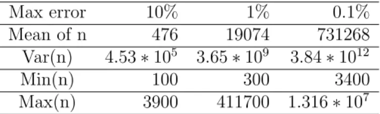
We want to see how many values need to be generated in order to get the estimated expected value and variance to within acceptable limits. We will setλ = 1,ϕ = 2, and then test how many values need to be generated for the estimates to have maximum error 10%, 1%, and 0.1%. 50 trials will be run in each case, and the mean, variance, and minimum and maximum values ofn will be recorded.
Results For podcheck1: Max error 10% 1% 0.1% Mean of n 476 19074 731268 Var(n) 4.53∗105 3.65∗109 3.84∗1012 Min(n) 100 300 3400 Max(n) 3900 411700 1.316∗107
Table 4: Descriptive statistics for number of values generated with function pod-check1 For podcheck2: Max error 10% 1% 0.1% Mean of n 416 26402 601526 Var(n) 2.07∗105 5.37∗109 1.70∗1012 Min(n) 100 900 2900 Max(n) 2900 502200 6341100
Table 5: Descriptive statistics for number of values generated with function pod-check2
Interpretation, Explanation
There does not appear to be any significant difference in the efficiency of these two codes. The most striking thing about these results is the enormous variability in
n. With acceptable error 10%, the minimum n was 100 for both functions, which is the number of values generated in each cycle, and thus the smallest possible n. For error 10%, the maximum and minimum value vary by an order of magnitude; for 1% and 0.1%, the maximum and minimum vary by at least 2−3 orders of magnitude. The minimum n for error 0.1% is comparable to the maximum n for error 10% in both cases. Until this process is better understood, it appears that this is a rather poor way of estimating necessary sample sizes, due to the extreme degree of variation.
Simulation 4: Compound overdispersed Poisson model Assumptions
Finally, we would like to test the validity of the compound overdispersed Poisson model. Using equations (13) and (14), we can predictEYi andV arYi, the expected
value and variance of the ith policy in a portfolio. We can then write a code that computes these values experimentally, using a given distribution Z of insurance claim sizes. In this way, we can see how the accuracy of the model increases with the number of policies n.
For these tests, we will not consider policies with different durations, since when
EZ and V arZ are known and λ, ϕ are fixed, then EYi and V arYi are linearly
proportional to ti. Therefore, the mean and variance will vary across policies in a
way that is strictly predictable. Test description
First, we will choose a model for insurance claim amounts. We will consider the Uniform, Lognormal, Normal, and Gamma distributions, and use two different sets of parameters for each. All parameters will be chosen so that the average claim amount EZ = 1000, in order to make comparison between models simpler.
parameters so that this possibility is sufficiently improbable as to be ignored. For each model, we will use m = 50 runs per test. We will consider ϕ = 1.01, 2, 3, and n = 100, 1000, 10000. In all cases, we will take the rate parameter λ = 1. For each test, we will find:
• The estimate of the policy mean and variance (denoted EYd, V arY\),
• The average absolute error of the expected value of the policy claim amount
1 m m P i=1 |EYd−EY| (denoted AD)
• The average absolute error of the above in the cases when EY < EYd and the number of trials for which this is the case (denotedAD−and m−
respec-tively), and the same for the cases when EY > EYd (denoted AD+ and m+,
respectively). Results Test 1: Z ∼U(500,1500) n ϕ EYd V arY\ AD AD− m− AD+ m+ 100 1.01 992.556 1079596.301 24.739 26.819 30 21.618 20 2 1006.172 2109961.582 22.920 22.036 19 23.461 31 3 1002.576 3103795.872 26.965 25.405 24 28.404 26 1000 1.01 999.177 1091868.621 6.916 7.442 26 6.347 24 2 999.566 2081527.638 6.086 6.269 26 5.888 24 3 999.604 3080988.066 6.230 5.917 28 6.629 22 10000 1.01 999.946 1093331.042 2.550 2.504 26 2.599 24 2 1000.341 2084822.417 2.278 2.105 23 2.425 27 3 1000.355 3085682.546 2.241 2.050 23 2.403 27
Table 6: Compound overdispersed Poisson model with uniformly distributed claims.
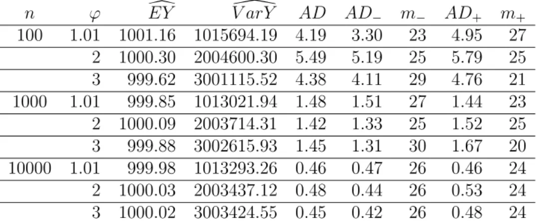
Test 2: Z ∼U(900,1100) n ϕ EYd V arY\ AD AD− m− AD+ m+ 100 1.01 1001.16 1015694.19 4.19 3.30 23 4.95 27 2 1000.30 2004600.30 5.49 5.19 25 5.79 25 3 999.62 3001115.52 4.38 4.11 29 4.76 21 1000 1.01 999.85 1013021.94 1.48 1.51 27 1.44 23 2 1000.09 2003714.31 1.42 1.33 25 1.52 25 3 999.88 3002615.93 1.45 1.31 30 1.67 20 10000 1.01 999.98 1013293.26 0.46 0.47 26 0.46 24 2 1000.03 2003437.12 0.48 0.44 26 0.53 24 3 1000.02 3003424.55 0.45 0.42 26 0.48 24
Table 7: Compound overdispersed Poisson model with uniformly distributed claims.
Test 3: Z ∼LN(1,3.43737)
For the Lognormal distribution with parameters mu, sigma, EZ =eµ+σ2
2 . Thus,
setting EZ = 1000 and choosing a value of µ, we can find the corresponding
σ. n ϕ EYd V arY\ AD AD− m− AD+ m+ 100 1.01 423.36 19183009.52 684.37 716.48 44 448.86 6 2 1466.22 3234237516.86 1640.45 667.18 44 8777.77 6 3 988.08 559588677.70 1165.54 717.96 41 3204.51 9 1000 1.01 701.86 397267858.15 495.06 521.84 38 410.26 12 2 1055.38 1189416265.59 661.09 432.65 35 1194.12 15 3 963.65 1090452568.81 748.12 530.04 37 1368.81 13 10000 1.01 833.39 1303942019.75 340.75 309.36 41 483.73 9 2 886.35 4245883236.55 400.74 313.65 41 797.48 9 3 913.72 5567767010.65 371.12 265.92 43 1017.31 7
Table 8: Compound overdispersed Poisson model with lognormally distributed claims.
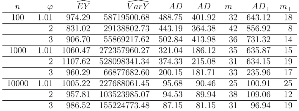
Test 4: Z ∼LN(4,2.411537) n ϕ EYd V arY\ AD AD− m− AD+ m+ 100 1.01 974.29 58719500.68 488.75 401.92 32 643.12 18 2 831.02 29138802.73 443.19 364.38 42 856.92 8 3 906.70 55869217.62 502.84 413.98 36 731.32 14 1000 1.01 1060.47 272357960.27 321.04 186.12 35 635.87 15 2 1107.62 528098341.34 374.33 215.08 31 634.15 19 3 960.29 66877682.60 200.15 181.71 33 235.96 17 10000 1.01 1005.22 227688061.45 95.68 90.46 25 100.91 25 2 957.81 103523985.07 94.53 89.94 38 109.06 12 3 986.52 155224773.48 87.15 81.15 31 96.94 19
Table 9: Compound overdispersed Poisson model with lognormally distributed claims. Test 5: Z ∼N(1000,100) n ϕ EYd V arY\ AD AD− m− AD+ m+ 100 1.01 999.06 1018183.71 7.18 7.51 27 6.78 23 2 999.15 2006699.08 8.07 7.68 29 8.60 21 3 1000.39 3012376.17 7.53 6.38 28 9.00 22 1000 1.01 1000.56 1021120.10 2.84 2.59 22 3.04 28 2 1000.19 2010835.66 2.48 2.39 24 2.57 26 3 999.86 3009189.38 2.57 2.81 24 2.34 26 10000 1.01 999.84 1019688.96 0.78 0.73 32 0.85 18 2 999.85 2009410.02 0.74 0.79 28 0.68 22 3 1000.09 3010548.16 0.92 0.86 24 0.97 26
Table 10: Compound overdispersed Poisson model with normally distributed claims.
Test 6: Z ∼N(1000,200) n ϕ EYd V arY\ AD AD− m− AD+ m+ 100 1.01 1001.81 1054584.49 15.31 13.50 25 17.13 25 2 998.46 2033977.59 15.72 15.41 28 16.12 22 3 1003.65 3063658.92 15.75 13.15 23 17.97 27 1000 1.01 1001.96 1054178.32 4.01 3.65 14 4.15 36 2 999.12 2036389.35 4.30 4.79 27 3.72 23 3 999.67 3037805.07 4.77 5.09 25 4.44 25 10000 1.01 1000.23 1050569.46 1.45 1.32 23 1.55 27 2 1000.38 2041642.57 1.62 1.18 26 2.09 24 3 1000.38 3042373.00 1.81 1.69 21 1.89 29
Table 11: Compound overdispersed Poisson model with normally distributed claims. Test 7: Z ∼Γ(20,50) n ϕ EYd V arY\ AD AD− m− AD+ m+ 100 1.01 999.55 1058903.10 14.12 16.56 22 12.21 28 2 998.96 2044765.42 14.95 15.37 26 14.50 24 3 1000.43 3053696.86 17.32 17.59 24 17.07 26 1000 1.01 1001.77 1064096.47 5.60 4.35 22 6.58 28 2 998.95 2046230.25 4.55 4.37 32 4.87 18 3 999.08 3044202.52 6.11 6.75 26 5.41 24 10000 1.01 1000.17 1060289.89 1.67 1.63 23 1.71 27 2 1000.05 2050205.38 1.67 1.68 24 1.66 26 3 1000.54 3053333.79 1.66 1.33 21 1.90 29
Table 12: Compound overdispersed Poisson model with Gamma distributed claims.
Test 8: Z ∼Γ(40,25) n ϕ EYd V arY\ AD AD− m− AD+ m+ 100 1.01 998.61 1032810.55 12.69 13.04 27 12.29 23 2 1000.60 2027749.67 11.23 9.84 27 12.86 23 3 996.21 3002873.15 14.73 14.46 32 15.19 18 1000 1.01 999.70 1034620.35 3.71 4.36 23 3.16 27 2 999.44 2022680.20 3.85 3.55 31 4.33 19 3 998.78 3017705.92 3.53 4.10 29 2.80 21 10000 1.01 999.54 1034041.47 1.53 1.50 33 1.59 17 2 1000.24 2025927.39 1.49 1.36 23 1.60 27 3 999.65 3023012.65 1.36 1.52 28 1.15 22
Table 13: Compound overdispersed Poisson model with Gamma distributed claims.
Interpretation, Explanation
For the Uniform distribution Z ∼ U(a, b), EYd was close to the theoretical value
EY = 1000, with a maximum error of less than 1%. The accuracy ofEYdimproved as n increased. For the variance, V arZ = (b−12a)2, so V arY = (a−12b)2 + 10002 ∗ϕ.
As such, we expected variances 1093333, 2083333, 3083333 for ϕ = 1.01, 2, 3, for the first set of parameters, and 1013333, 2003333, 3003333 for the second set. The calculated values were very close to these, increasing in accuracy as n
increased.
The absolute error terms decreased roughly by a factor of 3 whenn was increased by a factor of 10. This seems to indicate a practical lower bound for absolute error sizes based on portfolio size.
The results were similar when testing the Gamma- and Normally-distributed claims. The only troublesome case was for the Lognormally-distributed claims. EYd and
\
V arY varied wildly across tests, and accuracy improved only slightly as n in-creased. Average absolute error was extremely large, even for the largest values of n. Such high variability of the results can be explained by the huge variance of the proposed Lognormal models. In conclusion, while the compound overdispersed Poisson model appears to have held quite well for the other distributions tested, the Lognormal distribution with given parameters is not a viable choice.
¨
Ulehajuvusega mudelid kahjude arvu jaotuse
kirjeldamiseks
Magistrit¨
o¨
o (30 EAP)
Frazier Carsten
Kokkuv˜
ote
K¨aesoleva l˜oput¨o¨o peaeesm¨ark on uurida ¨ulehajuvusega mudeleid kindlustusport-felli kogukahju hindamiseks. T¨o¨o on jagatud kuueks osaks. Esimeses osas tutvus-tame l¨uhidalt t¨o¨o uurimisvaldkonda ja probleeme. T¨o¨o teises osas tuletame ja defineerime k˜oigepealt klassikalise kollektiivmudeli ning tuletame meelde tema olulisemad omadused. Seej¨arel keskendume Poissoni liitjaotuse mudelile, mis oma mitmete heade omaduste t˜ottu on ¨uks sagedamini kasutatavaid mudeleid.
T¨o¨o kolmandas osas ¨uldistame Poissoni liitjaotuse mudelit, lubades (erinevalt klas-sikalisest definitsioonist) poliisidele ka erineva pikkusega kindlustusperioode. N¨ai-tame ka, kuidas avalduvad suurima t˜oep¨ara hinnangud kirjeldatud mudeli para-meetritele.
Neljas osa keskendub ¨ulehajuvuse probleemile. Alustame ¨ulehajuvuse definit-siooniga ja v˜oimalike tekkep˜ohjustega, uurime ¨ulehajuvust t˜oen¨aosusjaotuse eks-ponentsiaalses peres ning n¨aitame, kuidas hinnata vastava mudeli parameetreid. L˜opuks n¨aitame, et klassikalise Poissoni mudeli aditiivsuse omadused j¨a¨avad keh-tima ka ¨ulehajuvusega Poissoni mudeli korral.
Viies osa tutvustab l¨uhidalt ¨uldisi v˜oimalusi ¨ulehajuvuse k¨asitlemiseks. Tutvus-tame Poissoni segamudeleid, millest tuntuim on negatiivse binoomjaotuse mudel, ja anal¨u¨usime, kas ja kuiv˜ord Poissoni mudeli head omadused nende mudelite kor-ral kehtima j¨a¨avad.
Magistrit¨o¨o kuuendas osas uurime teoreetilises osas defineeritud mudelite k¨aitumist simuleeritud andmete peal. Esiteks pakume v¨alja ¨uhe v˜oimaluse, kuidas negatiiv-se binoomjaotunegatiiv-se abil genereerida juhuslikke v¨a¨artusi etteantud parameetritega ¨
ulehajuvusega Poissoni mudelist. Teises simulatsioonis vaatleme ¨ulehajuvusega Poissoni mudeli aditiivsuse omadust. Seej¨arel uurime, milline on piisav valimi suu-rus ¨ulehajuvusega Poissoni mudeli parameetrite arvutamiseks etteantud t¨apsusega. L˜opetuseks anal¨u¨usime ¨ulehajuvusega Poissoni liitjaotusega mudeli k¨aitumist eri-nevate ¨uksikkahjude jaotuste korral.
T¨o¨o lisades on toodud m˜onede lemmade t˜oestused ja t¨o¨o praktilises osas kasutatud programmide tekstid.
References
1. Gray, R.J. & Pitts, S.M. (2012) Risk Modelling in General Insurance. From Principles to Practice. Cambridge University Press.
2. Hilbe, Joseph M. (2007) Negative Binomial Regression. Cambridge Univer-sity Press, New York.
3. K¨a¨arik, M. & Kaasik, A. (2012) On Premium Estimation Using the C&RT/Poisson Model and its Extensions. Lithuanian Journal of Statistics, 51(1), 5-13.
4. Quaintance, J. (2010) Combinatorial Identities: Table I: Intermediate Tech-niques for Summing Finite Series. (1.78), (6.1)
5. Tutz, G. (2012) Regression for Categorical Data. New York: Cambridge University Press. pp. 133-134.
Appendices
A
Proofs
Proof of equations (1) and (2): The function
MS(t) =E(etS),
Is called the Moment Generating Function (MGF) of random variable S. The moments of S are determined by:
E(Sn) =MS(n)(0),
Where MS(n) is the nth derivative of the function. First, we need to find a way to express MS(t) in terms of MN and MZ.
We know that S = PN
j=1
Zj. The Law of Total Expectation tells us that E(etS) =
E(E(etS|N)), where E(A|B) is the conditional expectation of A with respect to
B. Using our definition of S in terms of Zj, we see that:
E(E(etS|N)) =E(E(etZ)N) =E(MZ(t)N) =E(elnMZ(t)N) =MN(lnMZ(t)). Finally, MS(t) =MN(lnMZ(t)). (21)
To derive equation (1), we take the first derivative of the MS(t) using the chain
rule: MS(1)(t) =MN(1)(lnMZ(t))· MZ(1)(t)
t= 0. Note that MX(0) =E(X0) =E(1) = 1, so: MS(1)(0) =MN1(ln 1)·M (1) Z (0) 1 =MN(1)(0)·MZ(1)(0) =EN ·EZ.
To derive (2), we take the second derivative of MS(t). This becomes:
MS(2)(t) =MN(2)(lnMZ(t))· MZ(1)(t)2 MZ(t)2 +MN(1)(lnMZ(t))· MZ(t)·MZ(2)(t)−M (1) Z (t)2 MZ(t)2
Takingt= 0 once again, we find thatE(S2) =E(N2)·(EZ)2+EN·V arZ. Using
the formula for variance V arX =E(X2)−(EX)2, we find that: V arS=EN ·V arZ+ (EZ)2·V arN.
Proof of Proposition 2.1: We will prove the proposition by induction. For n = 1, the solution is trivial: N = N1 is Poisson distributed with parameter λ = λ1.
For n = 2, consider two independent Poisson random variables N1 and N2, with
parameters λ1, λ2, and let N = N1 +N2. We construct an argument based on convolutions: If N = z, then we can say that N1 = k and N2 = z−k, for some appropriately chosen value(s) of k. Since N1, N2 must be nonnegative integers, then clearly k may take any integer value from 0 to z. Thus, the convolution of
these distributions is: P(N =z) =P(N1+N2 =z) = z X k=0 P(N1 =k, N2 =z−k) = z X k=0 P(N1 =k)P(N2 =z−k) = z X k=0 e−λ1(λ1)k k! · e−λ2(λ2)z−k (z−k)! =e−(λ1+λ2)· z X k=0 λk 1λz2−k k!(z−k)! = e −(λ1+λ2) z! · z X k=0 λk 1λz −k 2 z! k!(z−k)! = e −(λ1+λ2) z! · z X k=0 z k λk1λz−k 2
We recognize the sum as the binomial expansion of (λ1 + λ2)z, so at last we
get:
P(N =z) = ((λ1+λ2))
ze−(λ1+λ2)
z!
This is clearly a Poisson random variable with intensity λ1+λ2. Thus, the sum of two independent Poisson random variables is still a Poisson random variable, with parameter equal to the sum of the component parameters. As an inductive assumption forn =m, suppose thatN1, . . . , Nm are independent Poisson random
variables with parameters λ1, . . . , λm, and that N = N1 +· · ·+Nm is a Poisson
random variable with parameter λ1 +· · · +λm. Then, for n = m + 1, N′ =
N1 +· · ·+Nm +Nm+1 = N +Nm+1 (due to our inductive assumption). This
is clearly still a Poisson random variable, with parameter λ′ = λ1 +· · ·+λ
m+1,
B
Program codes
All programs have been written in R.
Function for generatingnoverdispersed Poisson variables using Negative Binomial random numbers:
rpois.od=function(n,lambda,phi){ p=1/phi
alpha=lambda*p/(1-p)
#We determined these values for p and alpha algebraically. r=rnbinom(n,prob=p,size=alpha)
return(r) }
We use this function frequently in the practical section of this thesis. Functions for generating mean and variance to within a given accuracy:
podcheck1=function(lambda,phi,meanerror,varerror){ n0=100 #How many values we compute each cycle. n=0
meanerr=1 #We set this number to force the cycle to start. sum_Z=0
sum_Z2=0
while(abs(meanerr)>meanerror){
varerr=1 #We set this number to force the cycle to start. while(abs(varerr)>varerror){
n=n+n0 #The total number of values generated. Z=rpois.od(n0,lambda,phi) sum_Z=sum_Z+sum(Z) sum_Z2=sum_Z2+sum(Z**2) variance=sum_Z2/(n-1)-(sum_Z/n)**2 varerr=phi*lambda-variance }
}
phi=variance/(sum_Z/n)
return(c(sum_Z/n,variance,phi,meanerr,varerr,n)) }
This function generates 100 overdispersed Poisson values at a time. First, it gener-ates enough values to get the error of the variance to within an acceptable margin of error, and then generates additional values to do the same for the mean. It then checks whether the variance is still within acceptable limits given the additional values generated. If both mean and variance are acceptable, it returns these val-ues, as well as ϕ, the final error for mean and variance, and the total number of values generated.
podcheck2=function(lambda,phi,meanerror,varerror){ n0=100 #How many values we compute each cycle n=0
varerr=1 #We set this number to force the cycle to start. sum_Z=0
sum_Z2=0
while(abs(varerr)>varerror){
meanerr=1 #We set this number to force #the cycle to start
while(abs(meanerr)>meanerror){
n=n+n0 #The total number of values generated. Z=rpois.od(n0,lambda,phi) sum_Z=sum_Z+sum(Z) sum_Z2=sum_Z2+sum(Z**2) meanerr=lambda-sum_Z/n } variance=sum_Z2/(n-1)-(sum_Z/n)**2 varerr=phi*lambda-variance } phi=variance/(sum_Z/n) return(c(sum_Z/n,variance,phi,meanerr,varerr,n)) }
This code works the same way as the code above; however, it first calculates the mean, and then the variance.
Lastly, the following code generated the values used in Simulation 4.
compound_pod=function(n,phi,randtype,param1,param2){
lambda=1#We can adjust the time period so that this is true. sumclaimmean=0
#The sum of the average portfolio claim sizes sumabsdiff=0
#The sum of the absolute value of the difference #between actual and expected portfolio claim sizes sumabsless=0
#The sum of the above absolute values when actual #was less than expected
nless=0
#The number of cases when actual was less than expected sumabsmore=0
#The sum of the above absolute values when actual #was more than expected
nmore=0
#The number of cases when actual was more than expected sumclaimvar=0
#The sum of the portfolio claim size variance EY=1000
#The theoretical average portfolio claim size, since #EZ=1000 and EY=EZ*lambda=1000*1
m=50 #Number of trials for(i in 1:m){
claimnos=rpois.od(n,lambda,phi)
#The number of claims in each of the n policies. claims=randtype(n=sum(claimnos),param1,param2) #The size of each claim.
sumabsdiff=sumabsdiff+abs(lambda*mean(claims)-EY) if(lambda*mean(claims)>EY){ sumabsmore=sumabsmore+abs(lambda*mean(claims)-EY) nmore=nmore+1 } if(lambda*mean(claims)<EY){ sumabsless=sumabsless +abs(lambda*mean(claims)-EY) nless=nless+1 } sumclaimmean=sumclaimmean+lambda*mean(claims) sumclaimvar=sumclaimvar+lambda*(var(claims) +phi*(mean(claims)**2)) } portmean=sumclaimmean/m portvar=sumclaimvar/m
#Policies are independent, so the sum of their #variances is the portfolio variance.
return(c(portmean,portvar,sumabsdiff/m,sumabsless/nless, nless,sumabsmore/nmore,nmore))
}
Generating the data for a given test (e.g., test 1) was done as follows:
n=c(100,1000,10000) phi=c(1.01,2,3) param1=500 param2=1500 for(i in 1:length(n)){ for(j in 1:length(phi)){ print(round(compound_pod(n[i],phi[j],runif, param1,param2),digits=2)) } }
Non-exclusive licence to reproduce thesis and make thesis public
I, Frazier Carsten
(date of birth: November 6, 1987),
1. herewith grant the University of Tartu a free permit (non-exclusive licence) to:
1.1. reproduce, for the purpose of preservation and making available to the public, including for addition to the DSpace digital archives until expiry of the term of validity of the copyright, and
1.2. make available to the public via the web environment of the University of Tartu, including via the DSpace digital archives until expiry of the term of validity of the copyright,
Overdispersed Models for Claim Count Distribution, supervised by Meelis Käärik,
2. I am aware of the fact that the author retains these rights.
3. I certify that granting the non-exclusive licence does not infringe the intellectual property rights or rights arising from the Personal Data Protection Act.