Examining credit card consumption pattern
Yuhao Fan
(Economics Department, Washington University in St. Louis)
Abstract: In this paper, I analyze the consumer’s credit card consumption data from a commercial bank in China. To do so, I refer to the SMC model proposed by Schimittlein et al. in 1987.
I am proposing an extension to the model to incorporate the credit
card spending amount into the model. I
use transaction frequency, recency (defined as how recent a customer has used the credit card) and spending amount data to model consumer credit card consumptions and estimate parameters with the data. I get reliable estimates from the model. I introduce a value measure that is less informative but easier to compute than traditional CLV measures, to measure consumers’ contribution to the credit card issuer (the value of credit cards). I define the value measure of a credit card as the expected spending amount next month conditional on the card still active in this month. I further regress the value measures against the characteristics information of consumers and credit card to examine which characteristics information are the best predictors of values of the credit cards. I find that characteristic information is not useful estimates of the value measure of a credit card. Rather, the on-going value of a credit card is best explained by prior consumption records.Keywords: credit card consumption, Pareto/NBD “counting your customers” model, recency, frequency, purchase amount
1. This is my Senior Honor Thesis, and I am working with Professor Antinolfi in the Introduction Economics Department of WUSTL.
1. Introduction
Understanding consumption pattern is important for customer relationship management. This understanding allows firms to discriminate among consumers and make strategic marketing plans. For example, Kumar et al (2008) report that IBM keeps scores on their customers’ historical behaviors and use these scores to take marketing actions.
In both industry and academia, there has been great interest to develop models to predict consumption patterns. The SMC Model proposed by Schmittlein et al. (1987) is the earliest model, with a few extensions to the model proposed by other authors. Schmittelein et al. (1987) assume that purchases of each customer occur at random times and follow a Poisson process. The customers may drop out of the market randomly and the lifetime of the customers follows an Exponential distribution. Furthermore, they assume that heterogeneities of the parameters across the customers follow Gamma distributions. Under our assumptions, customers’ purchases show different patterns which are incorporated with different parameters, but these parameters are all from the same Gamma distributions and are thus connected. Although data on one single customer is limited, with a large population, we can still get accurate estimation of the parameters. Once we finish the model estimations, we can draw statistics of managerial relevance for marketing purpose, including the probability of being active at a certain point in time, expected lifetime, one-year survival rate, and expected number of transactions in a future period. The model has a number of successful applications. For example, Fader et al. (2005) study the e-commerce transactions over 78 weeks; Abe (2009) examines the shopping records for the members of a frequent shopper program at a department store in Japan for 52 weeks starting from July 1, 2000.
My data is from a commercial bank in China. It records its consumers’ credit card purchase behaviors and characteristics information of its consumers and the cards issued. In this paper, I use the model to examine consumers’ credit consumption patterns. To my knowledge, this is the first attempt to examine credit card consumption patterns with the SMC model. The model mentioned above focuses on the recency (defined as the most recent purchase of the card) and frequency of the purchases. They do not account for spending amount of each purchase. Without doubts, spending amount is very important to understand consumers’ consumption patterns and each consumer’s contribution to firms’ profits. Moreover, unlike the previous models, my data have information about the lifetime of each credit card. We know the exact lifetime of a credit card if it is cancelled before the end of sample period; or we know that the card is still valid at the end of the sample period. To analyze the data, I extend the model to accommodate these features.
With the data, I want to check the credit card consumption pattern both on aggregate and individual levels, and study the relationship between the consumption pattern and characteristics of the credit cards and their holders. By fitting the model to the data, I get the values of parameters which tell us the expected purchase frequency conditional on the activity of credit cards, expected spending amount of each purchase, and expected lifetime of each credit card.All of this information relates to the values of credit cards to the firm. To get a measure credit card’s contribution to the bank’s profits, I define the “value measure” of the credit card as the expected spending amount for the next month conditional on the
activity of the card, as the value measure of a credit card. To check whether the characteristics of credit cards and those of their users help identify the value of credit cards, I regress the parameters purchase frequency, dropout rate and the value measure on the characteristics of the credit card and those of its holders, including gender, education level, card level, promotion, and sale channel.
I have got some interesting results that are useful to improve customer relationship management. In aggregate, the expected lifetime of a typical credit card is estimated to be 101 months, expected number of purchases in a month for a typical credit card is 2.72, and expected spending amount in one purchase is 283 RMB (the currency in China, roughly equal to 45 dollars). On the individual level, I also get estimated values for the parameters, which reveal expected lifetime, expected number of purchases, and expected spending amount for each credit card. As a comprehensive value measure of credit cards, I also obtain the expected spending amount next month conditional that a credit card is currently active. The parameters and value measure for individual credit cards vary a lot, and they are good references to distinguish credit cards for marketing purpose. I also find that the characteristics of credit cards and their users show little information about credit card consumptions. To predict credit cards’ consumption in the future, past consumption record and the level of credit card are the most important information.
2. Literature Review
Based on the information about the recency and frequency of the purchases, several models have been developed to predict purchase patterns. Schmittlein et al. (1987) proposed the SMC model. The SMC model makes use of the recency and frequency of purchases by each customer, and is also referred to as the Pareto/NBD model. Key assumptions are the following: Purchases of each customer occur at random time and follow a Poisson process; the customers may drop out of the market randomly, and the lifetime of a customer follows an Exponential distribution; customers differentiate among each other with different parameters that guide the Poisson process and the Exponential distributions, and the parameters follow Gamma distributions.
Because the SMC model is difficult to implement, Fader et al. (2005) make an amendment to the model. Instead of assuming that the lifetime of a customer follows an Exponential distribution, they suppose that a customer drops out of the market after a purchase with probability 𝑝, and stays in the market with probability 1 − 𝑝 until the occurrence of the next purchase. To make the estimation of the parameters convenient, they assume a beta distribution for 𝑝 to incorporate the difference across customers.
Abe (2009) extends the SMC model in two ways: First, he uses Markov chain Monte Carlo (MCMC) to estimate the model parameters. Second, he relates model parameters to customers’ characteristics information, such as income, education, and location, which help distinguish customers from each other.
There is also an amount of large literature on credit card consumption. Mansfield, Pinto and Robb (2012) conduct a meta-analysis on credit cards. As they say, “the purpose of this study is to review and integrate the literature surrounding consumer credit cards in various disciplines and offer a series of guiding research opportunities to the marketing discipline.” They review 537 scholarly articles and categorize them into the following areas: (1)
consumers’ emotional response to credit cards, (2) consumers’ credit card behavior which mainly concerns about numbers of cards owned, balance, access/availability, repayment, and credit card misuse, (3)consumers’ knowledge or beliefs about credit cards. However, they haven’t mentioned any studies on evaluating the values of credit cards from the perspective of credit card issuers. This study tries to fill the gap.
3. Extension of the Model to accommodate features in the data 3.1. Model
In this section, I will review SMC model’s assumptions that I will follow and the assumptions I have to incorporate spending amount into the model. Then, I will write out the likelihood function and the steps of simulations to get the parameters we want.
The assumptions are as follow. We adopts the assumptions on the SMC model that a purchase with a credit card occurs at a random time and follows a Poisson process and the credit card may be cancelled randomly and its lifetime follows an Exponential distribution. We propose that natural log of spending amount in each purchase follows a Normal distribution. Customers differentiate among each other with random parameters that guide the Exponential distributions, the Poisson distributions, and the Normal distributions. In more details, let’s first review Schmittlein’s assumptions
(1) A credit card goes through two stages in its “lifetime”: it is active for some period of time, and then is cancelled and becomes permanently inactive.
(2) While active, the number of purchases made by a credit card follows a Poisson process with transaction rate 𝜆 ; thus the probability of observing 𝑥
transactions in the time interval (0, t] is given by
𝑃(𝑋(𝑡) = 𝑥|𝜆) =(𝜆𝑡)
𝑥𝑒−𝜆𝑡
𝑥! , 𝑥 = 0,1,2,3, …
And equally, the time between two purchases follows an Exponential distribution with 𝜆, and its probability density function is
𝑓(𝑡𝑗− 𝑡𝑗−1|𝜆) = 𝜆𝑒−𝜆(𝑡𝑗−𝑡𝑗−1).
(3) Observed “lifetime” 𝜏 of a credit card is Exponentially distributed with dropout rate 𝜇. The probability density function is
𝑓(𝜏|𝜇) = 𝜇𝑒−𝜇𝜏,
and thus the probability that the lifetime is longer than 𝑇 is
𝑅(𝑇|𝜇) = 𝑒−𝜇𝑇.
(4) Heterogeneity in transaction rates across credit cards follows a Gamma distribution with shape parameter 𝑟 and scale parameter 𝛼 as
𝑔(𝜆|𝑟, 𝛼) =𝛼𝑟𝜆𝑟−1𝛤(𝑟)𝑒−𝜆𝛼.
(5) Heterogeneity in dropout rates across credit cards follows a Gamma distribution with shape parameter s and scale parameter
𝑔(𝜇|𝑠, 𝛽) =𝛽𝑠𝜇𝑠−1𝛤(𝑠)𝑒−𝜇𝛽. We further make the assumptions that
(6) The natural log of the spending amount at 𝑗th purchase follows a Normal distribution as
log(𝑦𝑗) ~𝑁(𝜇𝑦, 𝜎𝑦2).
(7) Heterogeneity in the mean of the natural log of the spending amount, 𝜇𝑦, across
credit cards follows a Normal distribution as 𝜇𝑦~𝑁 (𝜇𝑦 𝑝
, (𝜎𝑦𝑝)2), and diversity of inverse of the variance, 1/𝜎𝑦2, across credit cards follows a Gamma distribution,
1/𝜎𝑦2~ ( 1 𝜎𝑦2) 𝛿0 2+1 exp (−𝛿1 2 1 𝜎𝑦2). 3.2. Model estimation Likelihood:
We observe that purchases occur at time 𝑡1, 𝑡2, …, 𝑡𝑥, with corresponding spending
amount 𝑦1, 𝑦2, …, 𝑦𝑥. If the card expires at time 𝜏, the likelihood of observing the sample
data given the parameters for the credit card is
𝐿(𝑡1, 𝑡2, … , 𝑡𝑥; log (𝑦1), log (𝑦2), …, log ( 𝑦𝑥); 𝜏|𝜆, 𝜇, 𝜇𝑦, 𝜎𝑦2)
= 𝜆 exp(−𝜆𝑡1) 𝜆 exp(−𝜆(𝑡2− 𝑡1)) … 𝜆 exp(−𝜆(𝑡𝑥
− 𝑡𝑥−1)) exp(−𝜆(𝜏 − 𝑡𝑥)) × 𝜇 𝑒𝑥𝑝(−𝜇𝜏) × 1 √2𝜋 1 (𝜎𝑦) 𝑥exp [− 1 2 ∑(log (𝑦𝑗) − 𝜇𝑦)2 𝜎𝑦2 ] = 𝜆𝑥exp (−𝜆𝜏)𝜇 exp(−𝜇𝜏) × 1 √2𝜋 1 (𝜎𝑦) 𝑥exp [− 1 2 ∑(log (𝑦𝑗)−𝜇𝑦)2 𝜎𝑦2 ].
Otherwise, if the card is still valid at time 𝑇, the end of the sample period, the likelihood of observing the sample data given the parameters for the credit card is
𝐿(𝑡1, 𝑡2, … , 𝑡𝑥; log (𝑦1), log (𝑦2), …, log ( 𝑦𝑥); 𝑇|𝜆, 𝜇, 𝜇𝑦, 𝜎𝑦2)
= 𝜆 exp(−𝜆𝑡1) 𝜆 exp(−𝜆(𝑡2− 𝑡1)) … 𝜆 exp (−𝜆(𝑡𝑥− 𝑡𝑥−1))
× exp(−𝜆(𝑇 − 𝑡𝑥)) × exp(−𝜇𝑇) × 1 √2𝜋 1 (𝜎𝑦) 𝑥exp [− 1 2 ∑(log (𝑦𝑗) − 𝜇𝑦)2 𝜎𝑦2 ] = 𝜆𝑥exp (−𝜆𝑇) exp(−𝜇𝑇) × 1 √2𝜋 1 (𝜎𝑦) 𝑥exp [− 1 2 ∑(log (𝑦𝑗)−𝜇𝑦)2 𝜎𝑦2 ].
Simulate 𝝀 for each credit card:
The posterior distribution of parameter 𝜆, having observed recency and frequency of purchases, is
𝐿(𝜆|𝑟, 𝛼, 𝑥, 𝜏) ∝ 𝜆𝑥exp (−𝜆𝜏)𝛼𝑟𝜆𝑟−1𝛤(𝑟)𝑒−𝜆𝛼∝ 𝜆𝑥+𝑟−1exp [−(𝜏 + 𝛼)𝜆]~𝐺𝑎𝑚𝑚𝑎(𝑥 + 𝑟, 𝜏 + 𝛼),
if the credit card is cancelled at 𝜏. The posterior distribution of parameter 𝜆 is
𝐿(𝜆|𝑟, 𝛼, 𝑥,𝑇) ∝ 𝜆𝑥exp (−𝜆𝑇)𝛼𝑟𝜆𝑟−1𝑒−𝜆𝛼 𝛤(𝑟) ∝ 𝜆
𝑥+𝑟−1exp [−(𝑇 + 𝛼)𝜆]~𝐺𝑎𝑚𝑚𝑎(𝑥 + 𝑟, 𝑇 +
𝛼),
if the credit card is valid at the end of sample period 𝑇. We simulate 𝜆 from 𝐺𝑎𝑚𝑚𝑎 (𝑥 + 𝑟, 𝜏 + 𝛼) or 𝐺𝑎𝑚𝑚𝑎(𝑥 + 𝑟, 𝑇 + 𝛼).
The posterior distribution of parameter 𝜇, having observed the credit card is cancelled at 𝜏, is
𝐿(𝜇|𝑠, 𝛽,𝜏) ∝ 𝜇 exp(−𝜇𝜏)𝛽𝑠𝜇𝑠−1𝛤(𝑠)𝑒−𝜇𝛽∝ 𝜇𝑠+1−1exp [−(𝜏 + 𝛽)𝜇]~𝐺𝑎𝑚𝑚𝑎(𝑠 + 1, 𝜏 + 𝛽). If the credit card is valid at the end of sample period 𝑇, the posterior distribution is
𝐿(𝜇|𝑠, 𝛽,𝑇) ∝ exp(−𝜇𝑇)𝛽𝑠𝜇𝑠−1𝛤(𝑠)𝑒−𝜇𝛽∝ 𝜇𝑠−1exp [−(𝑇 + 𝛽)𝜇]~𝐺𝑎𝑚𝑚𝑎(𝑠, 𝑇 + 𝛽).
We simulate 𝜇 from 𝐺𝑎𝑚𝑚𝑎(𝑠 + 1, 𝜏 + 𝛽) or 𝐺𝑎𝑚𝑚𝑎(𝑠, 𝑇 + 𝛽). Estimating parameters(𝒓, 𝜶):
When we have simulated values of {𝜆𝑖, 𝑖 = 1,2, … , 𝑁} for all credit cards, we
estimate(𝑟, 𝛼). Because we assume that 𝜆𝑖 follows the Gamma distribution with
parameters(𝑟, 𝛼), the joint likelihood of {𝜆𝑖, 𝑖 = 1,2, … , 𝑁} is
∏ 𝑔(𝜆𝑖|𝑟, 𝛼) = ∏ 𝛼𝑟𝜆 𝑖𝑟−1𝑒−𝜆𝑖𝛼 𝛤(𝑟) = 𝛼𝑁𝑟(∏ 𝜆 𝑖 ) 𝑟−1 𝑒−𝛼 ∑ 𝜆𝑖 (𝛤(𝑟))𝑁
We estimate (𝑟, 𝛼) by maximum likelihood. Estimating parameters(𝒔, 𝜷):
When we have simulated values {𝜇𝑖, 𝑖 = 1,2, … , 𝑁} of credit cards, we can
estimate(𝑠, 𝛽), the parameters in Gamma distribution which 𝜇𝑖 follows. The joint
likelihood of {𝜇𝑖, 𝑖 = 1,2, … , 𝑁} is ∏ 𝑔(𝜇𝑖|𝑠, 𝛽) = ∏ 𝛽𝑠𝜇 𝑖𝑠−1𝑒−𝜇𝑖𝛽 𝛤(𝑠) = 𝛽𝑁𝑠∏ 𝜇 𝑖 𝑠−1𝑒−𝛽 ∑ 𝜇𝑖 (𝛤(𝑠))𝑁
We estimate (𝑠, 𝛽) by maximum the likelihood.
Posterior distribution of (𝝁𝒚, 𝝈𝒚𝟐) for each credit card:
Because of diversity in the mean parameter, 𝜇𝑦 , and variance parameter, 𝜎𝑦2 , of the
natural log of spending amount among credit cards, we assume that for a randomly sampled credit card, 𝜇𝑦 follows a Normal distribution and 1/𝜎𝑦2 follows a Gamma distribution
respectively. That is 𝜇𝑦~𝑁 (𝜇𝑦 𝑝 , (𝜎𝑦 𝑝 )2), 1/𝜎𝑦2~ ( 1 𝜎𝑦2) 𝛿0 2−1 exp (−𝛿1 2 1 𝜎𝑦2).
The posterior distribution of mean 𝜇𝑦 for a credit card, having observed its spending
amounts, y1, 𝑦2, … , 𝑦𝑥 and given 𝜎𝑦2 known, is
𝐿(𝜇𝑦|𝑦1,𝑦2, …, 𝑦𝑥, 𝜎𝑦2) ∝ exp [− 1 2 ∑(log 𝑦𝑗−𝜇𝑦) 2 𝜎𝑦2 ] × exp [− 1 2 (𝜇𝑦−𝜇𝑦 𝑝 )2 𝜎𝑝2 ] ∝ 𝑁 ( ∑ log 𝑦𝑗 𝜎𝑦2 + 𝜇𝑦𝑝 𝜎𝑝2 𝑥 𝜎𝑦2+ 1 𝜎𝑝2 , 𝑥1 𝜎𝑦2+ 1 𝜎𝑝2 ).
We simulate 𝜇𝑦 for a credit card from 𝑁 (
∑ log 𝑦𝑗 𝜎𝑦2 + 𝜇𝑦𝑝 𝜎𝑝2 𝑥 𝜎𝑦2+ 1 𝜎𝑝2 , 𝑥1 𝜎𝑦2+ 1 𝜎𝑝2 ).
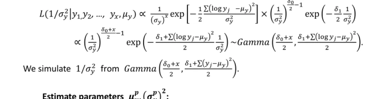
The posterior distribution of the inverse variance1/𝜎𝑦2 for a credit card, having observed
𝐿(1/𝜎𝑦2|𝑦1,𝑦2, …, 𝑦𝑥, 𝜇𝑦) ∝ 1 (𝜎𝑦) 𝑥exp [− 1 2 ∑(log 𝑦𝑗 −𝜇𝑦) 2 𝜎𝑦2 ] × ( 1 𝜎𝑦2) 𝛿0 2−1 exp (−𝛿1 2 1 𝜎𝑦2) ∝ (𝜎1 𝑦2) 𝛿0+𝑥 2 −1 exp (−𝛿1+∑(log 𝑦𝑗−𝜇𝑦) 2 2 1 𝜎𝑦2) ~𝐺𝑎𝑚𝑚𝑎 ( 𝛿0+𝑥 2 , 𝛿1+∑(log 𝑦𝑗−𝜇𝑦) 2 2 ). We simulate 1/𝜎𝑦2 from 𝐺𝑎𝑚𝑚𝑎 ( 𝛿0+𝑥 2 , 𝛿1+∑(𝑦𝑗−𝜇𝑦) 2 2 ). Estimate parameters 𝝁𝒚 𝒑 , (𝝈𝒚 𝒑 )𝟐:
After we have simulated values of 𝜇𝑦,1, 𝜇𝑦,2, … , 𝜇𝑦,𝑁, we estimate 𝜇𝑦 𝑝
, (𝜎𝑦𝑝)2 by maximizing the likelihood
𝐿(𝜇𝑦 𝑝 , (𝜎𝑦 𝑝 )2|𝜇𝑦,1, 𝜇𝑦,2, … , 𝜇𝑦,𝑁 ) ∝ 1 (𝜎𝑦𝑝)𝑁exp [− 1 2 ∑(𝜇𝑦,𝑖 −𝜇𝑦𝑝) 2 (𝜎𝑦 𝑝 )2 ]. Estimate parameters (𝜹𝟎, 𝜹𝟏):
After we have simulated values for 𝜎𝑦,12 , 𝜎𝑦,22 , … , 𝜎𝑦,𝑁2 , we estimate (𝛿0, 𝛿1) by
maximizing the likelihood
𝐿(𝛿0, 𝛿1|𝜎𝑦,12 , 𝜎𝑦,22 , … , 𝜎𝑦,𝑁2 ) = ∏ ( 1 𝜎𝑦,𝑖2 ) 𝛿0 2−1 exp (−𝛿1 2 1 𝜎𝑦,𝑖2 ) 𝑁 𝑖=1 . 4. Empirical evidence 4.1. Data summary
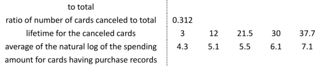
Table 1 is the summary statistics of credit card purchases. Our sample period is from 2008 to 2011, a total of 44 months, and the sample has consumption data for more than 10,000 credit cards. To make a preliminary analysis, we study the consumption data of the first 500 credit cards (data contains the consumption record of over 10,000 consumers and we use the first 500 consumers in the data for this analysis). Table 1 shows basic statistics of purchases with the credit cards. From the percentiles of the last purchase time, we can see that the median of the last purchase time is the 37th month and more than 25% credit cards have purchase records at the end of the sample period. From the statistics of the number of purchases, we find that the medium of number of purchases is 57. Over 5% of the credit cards have more than 374 times of purchases. However, the number of purchases is less than 13 for more than 25% credit cards, which means many credit cards are only used occasionally. We also see that around 14% of credit cards are not used at all, and around 31% are cancelled during the sample period. For the credit cards that have purchase record, the medium of the natural log of spending amount of each transaction is 5.5, which means that, on average, one purchase costs around 245 RMB.
Table 1. Simple statistics of credit cards
Percentile
5 25 50 75 95
Most recent purchase time (in months) 0 13 37 44 44
number of purchases 0 13 57.5 162 374.5
to total
ratio of number of cards canceled to total 0.312
lifetime for the canceled cards 3 12 21.5 30 37.7 average of the natural log of the spending
amount for cards having purchase records
4.3 5.1 5.5 6.1 7.1
4.2. Model estimation with the data
With the data, I proceed to estimate the model. First, initial values are given based on their relation to sample statistics of the data. For example, the expected time interval between two adjacent purchases is determined by 𝜆𝑖 as
𝐸(𝑡𝑗,𝑖− 𝑡𝑗−1,𝑖) = 1
𝜆𝑖 𝑗 = 1,2, … , 𝑥𝑖, for credit card 𝑖 = 1, 2, 3, … , 𝑁.
Thus 𝜆𝑖 is given an initial value of
𝜆̂𝑖 = 1 𝐸̂(𝑡𝑗,𝑖)= 1 1 𝑥𝑖∑ (𝑡𝑗,𝑖−𝑡𝑗−1,𝑖) 𝑥𝑖 𝑗=1 .
With the initial values of the parameters {(𝜆𝑖, 𝜇𝑖, 𝜇𝑦,𝑖, 𝜎𝑦,𝑖2 ), 𝑖 = 1,2, … , 𝑁}, we can simulate
and estimate all parameters iteratively using the methodology illustrated in section 3.2. We observe the convergence visually. We do a total of 5000 iterations. Then, we discard the first 2500 iterations and use the second 2500 to get the estimated values of the parameters. When doing the estimations, we find that the estimated values of parameters (𝑠, 𝛽)
remain unstable even after many times of iterations. After careful check on the data,I find that for each credit card, we only have one observation about the lifetime, 𝜏𝑖 or 𝑇𝑖. In this
situation, it is difficult to estimate both lifetime parameter 𝜇𝑖 and the parameters (𝑠, 𝛽)
that govern the heterogeneity in 𝜇𝑖among credit cards. Thus, I simplify the model by giving
𝑠 a value of 1. In this case, the Gamma distribution reduces to an Exponential distribution. The estimated parameters are shown in Table 2 and Figures 1 and 2.
Table 2. Estimated values of some parameters
𝑟 𝛼 𝛽 𝜇𝑦𝑝 (𝜎𝑦𝑝) 2 𝛿0 𝛿1 5 percentile 0.532 0.196 91.320 5.641 0.846 3.249 1.472 mean 0.558 0.205 101.249 5.647 0.852 3.505 1.634 95 percentile 0.583 0.214 111.638 5.653 0.859 3.768 1.802 Seeing the statistics in Table 2, we get a few important inferences at the aggregate level. We find that expected spending amount in one purchase for a typical customer is
exp(𝜇𝑦 𝑝
) = 283.44 RMB from estimated value of 𝜇̂𝑦 𝑝
, 5.647. From estimated value of 𝛽:
𝛽̂ = 101.249, we infer that the expected lifetime of a typical credit card is 101.249 months. From estimated values of 𝑟, 𝛼, we find that transaction rate of a typical credit card is 𝛼𝑟̂̂ = 2.7219, (because we have assumed the transaction rate follows a gamma distribution and mean of gamma distribution is 𝑟𝛼) which means the expected number of purchases for one typical credit card in 44 months is 2.7219 × 44 = 119. We also see that the estimated values for parameters {(𝜆𝑖, 𝜇𝑖, 𝜇𝑦,𝑖, 𝜎𝑦,𝑖2), 𝑖 = 1,2, … , 𝑁} in Figures 1, 2 vary a lot across
credit cards, and thus it is helpful to distinguish credit cards and manage “customer lifetime value” (CLV) on a systematic basis.
Figure 1. Estimated 𝛌 and 𝛍 for each credit card (for the credit card that has no consumption record, we don’t estimate its 𝛌, and give it a value of zero in the figure. )
0 50 100 150 200 250 300 350 400 450 500 0 10 20 30 average of simulated 0 50 100 150 200 250 300 350 400 450 500 0.005 0.01 0.015 0.02 average of simulated
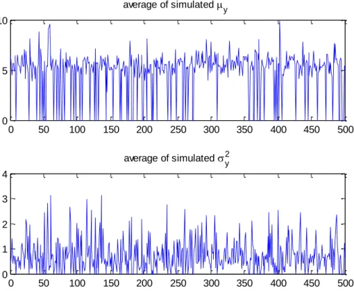
Figure 2. Estimated values for mean (𝝁𝒚,𝒊) and variance (𝝈𝒚,𝒊𝟐 ) of natural log of spending amount for
each credit card (for the credit card that has no consumption record, we don’t estimate the parameters, and give them a value of zero in the figure.)
Conditional on credit card 𝑖′𝑠 survival into next month, the expected total spending amount in the month is
E(number of purchases in one month × spending amount each time) = E(number of purchases in one month) ×
E(spending amount each time) = 𝜆𝑖× exp (𝜇𝑦,𝑖+ 𝜎𝑦,𝑖2
2 ).
The probability that the holder does not cancel the credit card the next month given that it is active now is
exp (−𝜇𝑖).
Thus the natural log of the expected spending amount with credit card 𝑖 the next month conditional that it is active now is
log 𝑄𝑖= log [exp (𝜇𝑦,𝑖+ 𝜎𝑦,𝑖2
2) × 𝜆𝑖× exp(−𝜇𝑖)] = 𝜇𝑦,𝑖+ 𝜎𝑦,𝑖2
2 + log(𝜆𝑖) − 𝜇𝑖.
Having estimated the parameters in the model, I calculate natural log of the expected spending amount log 𝑄𝑖, and use it to measure the value of each credit card. The higher
the measure, the higher value the credit card has. I calculate the value measure and plot it in Figure 3. For the credit cards that have no consumption record, I don’t estimate some of the parameters and assign their value measures as 0. The value measures take quite different values for different cards, and can help us distinguish credit cards for marketing 0 50 100 150 200 250 300 350 400 450 500 0 5 10 average of simulated y 0 50 100 150 200 250 300 350 400 450 500 0 1 2 3 4 average of simulated 2y
purpose.
Figure 3. Value measure (quality measure), log Q , of the credit cards
(For the credit card without purchasing records, the value is assumed to be zero. The value is reported in an increasing order.)
4.3. Test of the model assumptions
In our model, many assumptions are taken from previous studies and are taken as granted. For example, we follow the SMC model’s traditional assumptions that purchasing times of each credit card follow a Poisson distribution and the heterogeneity in purchase frequency across customers follow a Gamma distribution. We also propose new assumptions that the natural log of spending amount of each purchase follows a Normal distribution for each credit card and heterogeneities in means and variances of the Normal distributions across credit cards are described respectively by a Normal distribution and an inverse Gamma distribution. From Bayesian statistics, the distributions describing heterogeneities in means and variances come from the conjugate priors to make simulation simple. To demonstrate that the assumptions are reasonable and fit the data well, I test whether the spending amounts of all customers follow a Normal distribution here.
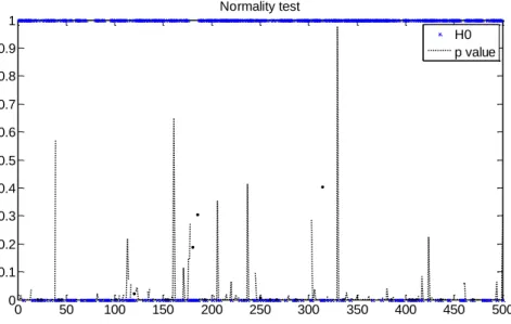
I perform a chi-square goodness-of-fit test for each credit card. The null hypothesis is that the spending amount of each purchase in the data follows a normal distribution at the 5% significance level. The results are reported in Figure 4. The null hypothesis is not rejected when H0 takes a value of 0; otherwise, H0 takes a value of 1 meaning that the normal distribution is rejected. P value is the probability of observing the given result if the null hypothesis is true. We see that fewer than one half credit cards are shown to follow Normal distributions. After a careful check, I find a possible reason for such a large number of rejections. Our data is observed monthly. We use monthly spending amount divided by the number of purchases in the month to represent the spending amount of each purchase. Thus, a consumer’s spending amount of each purchase in the same month is uniformly distributed. Even if the actual spending amount follows a normal distribution, the data behaves less likely to be from a normal distribution. Finally, although the real distribution of purchase amount for a credit card may be complicated, normal distribution is still a good approximation if we focus on first and second moments of the distributions.
0 50 100 150 200 250 300 350 400 450 500 0 2 4 6 8 10 12
Figure 4. Testing whether the purchase amount of a credit card follows a normal distribution. (H0=0 means normal distribution is accepted with 5% significance level; otherwise, H1=1 means it is rejected. p value is the probability of the sample happens when the normal distribution assumption is right. Some credit cards have no p values because of no sufficient observations to test. )
5. Relation between credit card purchase and characteristics of credit card and its holder
From the consumption data, I have estimated the model parameters and calculated the value measures of credit cards. I now check on the relation between them and characteristics of credit cards and their holders.
Table 3 shows the relation between purchase frequency parameter λ and characteristics of credit cards and their holders. Gender has no effect on purchase frequency. Education level1 has some effect, and highly educated credit card holders tend
to buy less frequently. Card level2 has a significant effect on purchase frequency. Holders of
a level-2 card purchase more frequently. Level-2 cards are “gold cards.” Only consumers with very good credit scores can apply for a gold card successfully.2
1 Education has 5 levels. Edu_h means that the holder graduated from high school. Edu_p means the
holder graduated from college, and edu_u means that holder graduated from university. Edu_m means the hold has a master degree or above. The base level is holder who graduated from middle school or below.
2 Level-1 card is called common card. Level-2 is gold credit, which is the most premium one among the
three. Level-3 card is called youth card for young people.
3 Baseline education means the card holder graduated from middle school. Edu_h means the card holder
graduated from high school. Edu_p means the holder graduated from junior college. Edu_u means the holder graduated from college. Edu_m means the holder has a master degree or PhD degree.
4 Baseline promotion is the promotional event for common and gold card in 2007. Promotion_2 is the
promotional event for youth card in 2007. Promotion_3 is the promotional event for common and gold card in 2008. Promotion_4 means the card was open without any promotions.
0 50 100 150 200 250 300 350 400 450 500 0 0.1 0.2 0.3 0.4 0.5 0.6 0.7 0.8 0.9 1 Normality test H0 p value
Definition of variables:
Education has 5 levels. Edu_h means that the holder graduated from high school. Edu_p means the holder graduated from technical schools, and edu_u means that holder graduated from university. Edu_m means the hold has a master degree or above. The base level is holders who have education level of 9th grade or below.
Level-1 card is called common card. Level-2 is gold cold, which is the most premium one among the three. (Banks usually only give gold card to customers with high incomes and good credit scores.) Level-3 card is called youth card for young people (people who are over eighteen but has no checking or saving accounts can apply for youth cards under the accounts of legal parents).
Baseline promotion is the promotional event for common and gold card in 2007. Promotion_2 is the promotional event for youth card in 2007. Promotion_3 is the promotional event for common and gold card in 2008. Promotion_4 means the card was open without any promotions.
Gender is a dummy variable. Male is assigned to be 1 and female is assigned to be 0. Age variable is the age at which the consumer opened the card.
Baseline channel level means the cards were opened at the branch banks. Channel_1 means the cards were opened through third-party stores. Channel_2 means the card were opened directly at the bank.
Table 3. Regressing 𝛌 on characteristics of credit card and its holders
constant 2.63 3.98 2.21 2.82 1.63 3.58 2.59 3.24 (11.10) (6.16) (10.55) (16.27) (7.26) (6.86) (4.17) (4.99) gender 0.16 (0.50) edu_h -2.80 -2.88 (-1.51) (-1.59) edu_p -1.44 -0.96 (-1.98) (-1.33) edu_u -1.84 -1.50 (-2.63) (-2.17) edu_m -0.81 -0.75 (-1.18) (-1.10) card_level2 1.75 1.64 (5.00) (4.79) card_level3 -0.06 (-0.13) promotion_2 -0.66 (-1.57) promotion_3 -1.66 (-0.47) promotion_4 1.74 (1.21) channel_2 -1.01
(-1.83) channel_3 -0.52 (-0.76) age 0.00 (0.22) R square 0.00 0.03 0.05 0.01 0.08 0.01 0.00 0.07 𝜇𝑦 is the expected natural log of spending amount for each purchase. Table 4 reports
the evidence of regressing 𝜇𝑦 on the characteristics of credit cards and their holders. We
see that gender, education level, and promotion have no obvious effect on the parameter. Card level has a positive effect, and sale channel has a minor effect. Gold cards (level 2) and youth cards (level 3) have higher spending amount for one purchase on average than level-1 cards, which are common cards.
Table 4. Regressing 𝛍𝐲on characteristics of credit card and its holder
constant 4.66 5.17 4.24 4.73 5.58 4.53 4.53 (31.69) (12.92) (33.14) (43.96) (17.32) (11.75) (19.65) gender 0.24 (1.20) edu_s 0.84 (0.73) edu_h -0.62 (-1.37) edu_p -0.74 (-1.70) edu_u -0.04 (-0.10) card_level2 1.38 1.34 (6.49) (6.22) card_level3 0.81 0.80 (3.09) (3.06) promotion_2 0.32 (1.23) promotion_3 0.94 (0.43) promotion_4 0.46 (0.51) channel_2 -0.91 -0.35 (-2.68) (-1.51) channel_3 -0.64 (-1.50) age 0.01 (0.69) R-sqaures 0.00 0.03 0.08 0.00 0.01 0.00 0.08
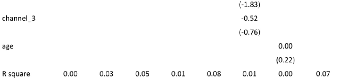
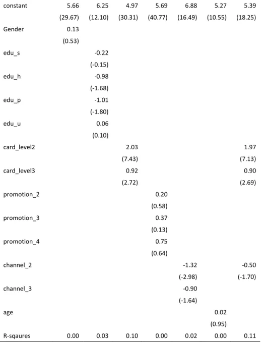
Finally I regress the credit card value measure log 𝑄, on the characteristics of credit cards and their holders and find the relation between them in Table 5. The evidence shows that card level affects the value measure. On average, gold cards have the highest value and youth cards contribute more value than common cards.
Table 5. Regressing log 𝑄 on characteristics of credit card and its holders
constant 5.66 6.25 4.97 5.69 6.88 5.27 5.39 (29.67) (12.10) (30.31) (40.77) (16.49) (10.55) (18.25) Gender 0.13 (0.53) edu_s -0.22 (-0.15) edu_h -0.98 (-1.68) edu_p -1.01 (-1.80) edu_u 0.06 (0.10) card_level2 2.03 1.97 (7.43) (7.13) card_level3 0.92 0.90 (2.72) (2.69) promotion_2 0.20 (0.58) promotion_3 0.37 (0.13) promotion_4 0.75 (0.64) channel_2 -1.32 -0.50 (-2.98) (-1.70) channel_3 -0.90 (-1.64) age 0.02 (0.95) R-sqaures 0.00 0.03 0.10 0.00 0.02 0.00 0.11 6. Conclusion
In the data on credit card consumption, number of purchases and total spending amount each month is observed. To make use of observations of spending amount, a critical information to evaluate credit card consumptions, I extend the models proposed by Schmittlein et al. (1987) and Abe (2009). I assume that natural log of spending amount of each credit card follows a Normal distribution, and diversity in the means and variances of the normal distributions across credit cards follow a Normal distribution and an inverse
Gamma distribution respectively. With the data, I get reliable estimated values of the parameters, which provide important information about the consumption pattern of each credit card and credit cards on aggregate level. For example, in aggregate, the expected lifetime of a typical credit card is estimated to be 101 months, expected number of purchases in a month is 2.72, and expected natural log of spending amount in one purchase is 6.4. The expected frequency and expected spending amount of each purchase varies a lot across credit cards. To evaluate credit cards with these estimated parameters, I introduce the expected spending amount for the next month conditional that the credit card is active now as a value measure of the credit card. The value measure varies much across credit cards and thus is helpful to distinguish values of credit cards. Finally by regressing the estimated parameters and the value measure on the characteristics of credit cards and their holders, I find that card level has a significant effect on credit card purchase patterns and other characteristics have no significant effects.
References
Abe Makoto. 2009. “Counting your customers” one by one: a hierarchical Bayes extension to the Pareto/NBD Model, Marketing Science, 28(3), 541-553.
Fader, P. S., B. G. S. Hardie, K. L. Lee. 2005a. Counting your customers the easy way: An alternative to the Pareto/NBD model. Marketing Science, 24(2), 275–284.
Fader, P. S., B. G. S. Hardie, K. L. Lee. 2005b. RFM and CLV: Using iso-value curves for customer base analysis. J. Marketing Res. 42(4), 415–430.
Mansfield P., Pinto M., and C. Robb. 2012. Consumer and credit cards: A review of empirical literature. Working paper, forthcoming in Journal of Management and Marketing Research
Schmittlein, D. C., D. G. Morrison, R. Colombo. 1987. Counting your customers: Who are they and what will they do next? Management Sci. 33(1), 1–24.