Three Essays in Education Finance

Three Essays in Education Finance

by

Regine Gail Lucasan

A dissertation submitted in partial fulfillment of the requirements for the degree of

Doctor of Philosophy (Economics)

in the University of Michigan 2018

Doctoral Committee:

Professor James Hines, Jr., Chair Professor John Bound

Professor Brian McCall Professor Joel Slemrod

Regine Gail Lucasan [email protected] ORCID: 0000-0001-7892-4500 c

ACKNOWLEDGEMENTS

I thank my chair, Jim Hines, for his guidance, support, and boundless optimism, with-out whom I could not have completed this dissertation. I thank Joel Slemrod, for always encouraging me to focus on details, but to not lose track of the bigger picture. I thank John Bound and Brian McCall, for their insight, patience, and generosity with their time. I will always be grateful to my fellow graduate students at the University of Michigan–couldn’t ask for a better group to have joined me on this journey.

TABLE OF CONTENTS

1.1 Introduction . . . 1

1.2 Background . . . 3

1.2.1 Prior literature . . . 3

1.2.2 State and local roles in K-12 public education finance . . . 5

1.3 Determining per-pupil revenues at state and local levels . . . 7

1.3.1 Choosing the level of state education revenues . . . 9

1.3.2 Choosing the level of district (local) education revenues . 13 1.3.3 Summary of model predictions . . . 16

1.4 Data . . . 17

1.5 Empirical framework . . . 18

1.5.1 First-differenced estimates . . . 19

1.5.2 IV estimation . . . 20

1.6 Results and Analysis . . . 22

1.6.1 Graphical analysis . . . 22

1.6.2 Testing the credibility of the instrumental variable approach 23 1.6.3 Estimation results . . . 23

1.7 Conclusion . . . 26

1.8 Figures . . . 28

1.9 Tables . . . 40

II. The Impact of the Great Recession on K-12 Public Education Finance . . 48

2.2 Institutional background . . . 50

2.2.1 K-12 education finance at the Federal level . . . 50

2.2.2 The American Recovery and Reinvestment Act . . . 51

2.3 Data and sample selection . . . 52

2.4 Estimation strategy . . . 53

2.4.1 The relationship of interest . . . 53

2.4.2 Instrumental variables . . . 55

2.4.3 Two-stage least squares estimation . . . 57

2.5 Results . . . 57

2.5.1 Effect of Federal stimulus funds on education finance . . . 57

2.5.2 Decomposition of results: existing vs. new programs . . . 60

2.6 Conclusion . . . 63

2.7 Figures . . . 65

2.8 Tables . . . 70

III. State Finance Systems and Crowding-out by State Contributions to Ed-ucation . . . 76

3.1 Introduction . . . 76

3.2 A brief history of state finance systems and reforms . . . 77

3.3 Properties of state education finance systems . . . 79

3.4 Data . . . 82

3.4.1 Data and sample selection . . . 82

3.4.2 Descriptive statistics . . . 83

3.5 Estimation strategy . . . 83

3.6 Results . . . 85

3.6.1 A visual analysis . . . 85

3.6.2 Crowd-out rates over time . . . 86

3.6.3 Event study analysis . . . 87

3.7 Conclusion . . . 89

3.8 Figures . . . 91

3.9 Tables . . . 95

LIST OF FIGURES

Figure

1.1 Growth of the U.S. foreign-born population . . . 28

1.2 Mean household income over time, by nativity of the head of household . 29 1.3 Share of K-12 education revenue by source . . . 30

1.4 Variation in total education spending . . . 31

1.5 State education funding systems, 2007 . . . 32

1.6 Preferred state tax rates . . . 33

1.7 The relationship between wealth and immigration . . . 34

1.8 Education revenue by source and income, 1970-2007 . . . 35

1.9 Education revenue by source and state contributions, 1970-2007 . . . 36

1.10 Immigration and education spending, 1970-2007 . . . 37

1.11 Immigration and education spending, shorter time periods . . . 38

1.12 Immigration and state and local revenue . . . 39

2.1 Time series of the share of K-12 education revenues by source . . . 65

2.2 Trends in per-pupil revenue during the Great Recession . . . 66

2.3 Effect of program instruments on Federal grants by year . . . 67

2.4 Effect of program instruments on existing (old) Federal grants by year . . 68

2.5 Effect of program instruments on new Federal grants by year . . . 69

3.1 State finance properties over time . . . 91

3.2 States and properties of the educational finance system, 2012 . . . 92

3.3 State revenues by source and state finance property . . . 93

LIST OF TABLES

Table

1.1 Summary of model predictions . . . 40

1.2 State revenue level regressions using OLS . . . 41

1.3 Local revenue level regressions using OLS . . . 42

1.4 IV credibility estimates . . . 43

1.5 IV falsification tests, 1965-1970 . . . 43

1.6 Estimates of effects on per-pupil state revenue, 1970-2007 . . . 44

1.7 Estimates of effects on per-pupil local revenue, 1970-2007 . . . 45

1.8 Robustness to excluding 2007: estimates of effects on per-pupil state rev-enue, 1970-2000 . . . 46

1.9 Robustness to excluding 2007: estimates of effects on per-pupil local rev-enue, 1970-2000 . . . 47

2.1 Allocation of Recovery Act education funds . . . 70

2.2 Summary statistics by quintile of recovery grants received . . . 71

2.3 First stage regressions . . . 72

2.4 Effect of (all) Federal grants . . . 73

2.5 First stage estimates of decomposition . . . 74

2.6 Second stage estimates of decomposition . . . 75

3.1 States and funding formula types, 2012 . . . 95

3.2 Frequency of combinations of state finance properties . . . 96

3.3 Summary statistics by state finance property . . . 97

3.4 Estimates of the crowd-out rate by state finance property . . . 98

ABSTRACT

My dissertation consists of three chapters in the field of education finance. In the United States, education is the joint responsibility of Federal, state, and local governments. I ex-plore the interactions between these different sources of funds and examine how these are affected by a variety of factors: immigration, policy changes, and education finance reform. I study state and local government education budgeting decisions, and build eco-nomic models that capture realities of public education financing when there are different but interrelated sources of funding. I use empirical analysis on extensive data on school district finances linked to demographics to evaluate the empirical implications of these models, and develop comprehensive measures of tax adjustments in public education fi-nance.

My first chapter offers an alternative interpretation of the negative relationship be-tween immigration flows and changes in per-pupil spending in U.S. school districts. I argue that fiscal channels are sufficient to explain the negative effect of immigration on education funding and decompose the effect into separate responses at different levels of government. Immigrants have lower incomes on average than natives, and so their immi-gration increases the cost to natives of providing uniform education. I find that while state contributions to education do not respond to immigration, local governments decrease education revenues by 7.4 percent for every 1 percentage point increase in immigration, or about $319 when evaluated at the 2007 average county education contribution. This corresponds to an estimated elasticity of -0.43. Thus, median voter politics largely in-sulate state governments from increases in the tax price of education in the presence of immigration, but do not do so for local governments.

My second chapter estimates the impact of Federal grant expansions during the Great Recession. During this period, the Federal government increased its contributions toward K-12 education by about 50%. I use an instrumental variable approach to estimate the ef-fect of these expanded Federal contributions on state and local district education finance, focusing on the extent of crowd-out. I find that the fiscal response to increased Federal funding is different at these two levels of government, and is dependent on the program through which the additional funds are channeled. Funds from expanded existing pro-grams like Title I and IDEA Special Education did not crowd out state and local district education contributions. These grants increased total revenue dollar for dollar. In sharp contrast, funds from the new State Fiscal Stabilization Fund completely crowded out state education contributions, leaving local district contributions unaffected.

My third chapter investigates the crowding out of increased state education contribu-tions on total education spending at the school district level and explores how the crowd-out rate relates to the states choice of education funding system. Using an event study framework, I find that different properties of education funding systems imply different

levels of redistribution within-state. State finance systems with properties that encourage equalization, like minimum foundation plans and spending limits, result in crowding-in of education funds by state contributions. On the other hand, properties like equalization plans and reward-for-effort plans result in crowding-out of funds.

CHAPTER I

Immigration, Fiscal Federalism, and the Tax Price of

Education

1.1

Introduction

The U.S. has seen rapid growth in immigration since the Immigration and Natural-ization Act of 1965 abolished immigration quotas, with the U.S. foreign-born population increasing four-fold (and share increasing three-fold) from 1970 to 2013 (Figure 1.1). A consequence of this growth is rising diversity in communities, which has been associated with declining support for public goods provision, particularly for public education. Much of the previous literature on this topic has focused on social mechanisms like ethnic frag-mentation (Alesina et al. (1999), Dahlberg et al. (2012)), in-group biases (Coen-Pirani (2011), Speciale (2012)) or cultural differences (Baldwin and Huber (2010)), but much less studied is how changing fiscal burdens induced by immigration may be driving this phenomenon.

In this paper, I argue that fiscal channels are sufficient to explain the negative effect of immigration on education funding and decompose the effect into separate state and local government responses. I develop a model that explicitly describes how immigration changes the tax price of education, which is the amount of additional taxes that have to be paid by the taxpayer in order to raise public education by $1. This change is not uniform in the separate jurisdictions, which allows me to provide a quantitative measure of how immigration impacts public education finance at different levels of government.

There are three major themes that emerge from this investigation. First, state and local governments do not respond equally to immigration. In the U.S., the responsibility1 _for

education funding is almost equally shared between state and local governments, which face different tax bases and different incentives when setting taxes. Because money is

1_{About 90% of all education revenues in 2014 are attributed to state and local governments. The}

fungible, past analyses using current spending in education as the outcome variable are unable to distinguish between these two responses. By focusing on education revenues instead of spending, I am able to find a better measure of how governments respond to immigration. Second, immigration into a district does not change the amount of per-pupil state aid that the district receives. This is because median voter politics implies that the choice of state contributions is made outside of the district, and that decision depends only on the relative magnitude of median district2_{income and mean state income. Third,}

immigrants tend to be poorer than natives (Figure 1.2), and so immigration into a district weakly increases the tax price of education which is the amount of taxes that has to be paid to raise the funding of public education by $1. Because education is now more expensive, the district reduces its per-pupil education funding contribution.

I model education spending as the solution to a two-stage optimization problem, which reflects how education revenues are raised in the vast majority of states. At the state level3_{, legislators decide on a minimum level of per-student education funding, called the}

foundation grant. At the local district level, each of the districts in the state can choose to augment the foundation grant by collecting local taxes subject to rules specified by state legislation.

The model describes how state and local tax revenues change in response to changes in immigration. The interaction between state and local governments’ funding decisions have implications for their ability to respond to immigration. Because there is a single state funding scheme, state legislators act to redistribute income within the state. The model predicts that state education revenues allocated towards a particular district are negatively related to district income, but are independent of the district’s immigrant share. On the other hand, local districts set their own tax rates, and wealthier districts are less constrained by the state minimum education requirement than poorer districts. The model predicts that district education revenues are positively related to district income, and are negatively correlated to immigration. Combining this with the observation that immigra-tion decreases total educaimmigra-tion revenue leads to the result that the effect of immigraimmigra-tion is concentrated at the local district level.

My empirical analysis exploits variation at the county level using decennial data from 1990-2007 to show the long-run impact of changes in immigration on education finance. Concerns about reverse causality due to Tiebout (1956) sorting or omitted variable bias are addressed by using an instrumental variable that is the predicted change in the fraction of

2_{The median district I refer to here is the median voter for the purposes of determining state contributions}

to education. Section 1.2 describes this in more detail.

3_{This describes how education funding works in most, but not all states. More details are provided in}

foreign-born residents based on historical immigrant settlement patterns, as done in Card (2001) and Wozniak and Murray (2012). The empirical analysis supports the theoretical predictions of the model. I show that the previously downward decrease in education spending that is associated with an increase in immigration into a district is due almost entirely to a decrease in education revenue raised by the local school district. This can be attributed to a substitution effect: immigrants to a district increase the local tax price of education by more than the increase in the state tax price, and so raising funds for education becomes relatively more expensive at the local level.

The rest of this paper is organized as follows. Section 1.2 describes the prior literature and the institutional background of U.S. public K-12 education finance. Section 1.3 intro-duces the model set-up and describes the implications of the model. Section 1.4 describes the data used to test the model implications. Section 1.5 and 1.6 present the empirical framework and analysis. Section 1.7 concludes.

1.2

Background

In this section, I describe the state of the literature on immigration and public educa-tion provision, and provide an introduceduca-tion to the institueduca-tional background of public K-12 education that informs the model set-up.

1.2.1 Prior literature

This paper is related to several strands of the literature on public goods. Specifically, it relates to the extensive work on population demographics as determinants of government spending on public goods. However, while this literature is extensive, in this paper I focus on immigration and explore the fiscal mechanism of its impact on public education finance. This paper is also unique in that it approaches this question from two perspectives, a theoretical, model-driven approach and an empirical approach.

The literature on demographics and public good provision shows that there are low lev-els of public good provision in heterogeneous and ethnically diverse societies. The seminal paper by Alesina et al. (1999) finds that individuals’ willingness to contribute to public goods depends on the racial composition of the community. In particular, the authors’ cross-sectional analysis shows that higher levels of racial fragmentation are associated with lower spending. There are several different mechanisms that have been proposed to explain this empirical result. Alesina and Ferrara (2005) describe in their review of the literature that perhaps different ethnic groups may differ in their preferences for public

goods, and so increased diversity results in an increased difficulty to agree on a common public policy or a common level of public good provision.

Hoxby (2001) finds that at the metropolitan statistical area (MSA) level, increased racial heterogeneity has a negative effect on education spending. La Ferrara and Mele (2006) subsequently showed that there is increased racial segregation at the level of school jurisdictions, implying that individuals are sorting within the MSA level into more racially homogeneous districts. They also find that racial segregation has a positive effect on av-erage per-pupil spending on education, but there is more inequality across districts in the same MSA. A related paper is Urquiola (2005), which finds that as districts become more racially distinct within MSAs, there is increased diversity in the levels of per-pupil spending in these districts.

Changing demand for public good provision is also induced by the changing age distri-bution as the baby boom population ages. Policymakers have long focused on the impact of aging populations on Federally-funded programs like Social Security and Medicaid, but state and local governments also have cause for concern. The literature suggests that the elderly vote to support their own interests, and so as populations age, the shifting political power from the working-age to the elderly could potentially lead to fewer resources being allocated toward public goods targeted for children, including education. The most influ-ential paper in this category is by Poterba (1998), who examined how intergenerational conflict has affected states’ willingness to fund public education. He finds that a high pro-portion of people over 65 in a state is associated with a lower amount of state spending on public education. He also finds the negative relationship is more pronounced in the states where older individuals are ethnically or racially different from those that are school-aged. Ladd and Murray (2001) analyze the same relationship at the county level and find a much smaller elasticity, due to more stringent controls to account for Tiebout bias. The elderly tend to move to counties with fewer children, and so even if at the state level they have a negative effect on education spending (the Poterba result), the effect is diminished at the county level.

There is a growing literature on the relationship between immigration and public goods spending. Bheim and Mayr (2005) use a model where natives derive less utility from immigrants’ use of public goods. Their empirical work uses data from OECD countries and find heterogeneous effects of vs low-skilled immigration. Specifically, while high-skilled immigration has a positive effect on public spending, the presence of anti-social effect means that low-skilled immigration has a negative effect on public spending.

In the United States, the education finance literature focuses primarily on the Mexican immigrant population or the traditional immigrant settlement states. Coen-Pirani (2011)

models education as a pure state public good and uses data from California to argue that a 19% decrease in education spending can be attributed to immigration. However, he does not account for the fact that in California a significant portion of spending is not determined at the state level, and so education spending is not completely equalized across the state. Furthermore, Mexican immigrants are a minority of all U.S. immigrants4_{, and so}

a more complete analysis of the impact of immigration should also include the foreign-born from countries other than Mexico.

Dottori et al. (2009) develop a theoretical model of how low-skilled immigration affects public education spending. The mechanism studied in their paper is the erosion of the tax base, coupled with an increased demand for private education and lower funding of public education. Similarly to the Coen-Pirani model, education is considered a state public good and local government responses are not considered in the authors’ analysis. Their paper is solely theoretical and does not contain an empirical section. By bringing data from an extended time period into my analysis, I am able to estimate a measure of the impact of immigration.

Finally, the most closely related paper to my empirical work is that by Speciale (2012). He analyzes the impact of immigration on the EU-15 countries using the distance from the Balkan wars as an instrument and finds a small negative effect of immigration on public education expenditures, an elasticity of -0.15. Similarly to Poterba and Ladd and Murray, he also suggests that the channel driving this result is that ethnically diverse societies may be valuing public goods lower than private goods. In contrast, my analysis is set in the U.S. and takes advantage of the extensive data that has been collected on state districts and demographics over a large time period, and my elasticity estimates fall within the range of the elasticity estimates in these earlier papers.

1.2.2 State and local roles in K-12 public education finance

In this subsection, I describe how states and local districts make the decision on how much public education funding to award to districts, and how that informs my theoretical model.

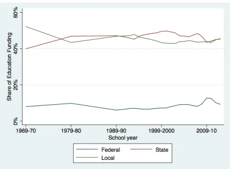
Education funding is a shared responsibility between Federal, state, and local govern-ments, but most of the burden lies with state and local governments. The state and local government share is about 90% compared to the Federal government’s 10%, and this di-vision has been stable over time, with a slight inclination toward more state spending.

4_{Mexican foreign-born people constitute about 28% of all foreign-born U.S. residents of 2014, and this}

number has been decreasing over time. Source: Migration Policy Institute’s ACS/Census data tool accessed at https://www.migrationpolicy.org/programs/data-hub/state-immigration-data-profiles.

Figure 1.3 shows the trend of education revenue by source.

The largest programs through which the Federal government funds education are No Child Left Behind Title 1 Grants, which are directed toward school districts via funding formulas based on student characteristics such as child poverty rates. The second largest program are Individuals with Disabilities Education Act (IDEA) Special Education Grants, which are allocated to districts according to child statistics relating to disabilities. Never-theless, education does not constitute a large fraction of the Federal government’s budget, with only $55.9 billion going K-12 education in 2013, approximately 1.4% of the total Federal budget that year. Furthermore, because most Federal education funding is tied to these formulas under current law, there is less scope for the Federal government to respond to immigration.

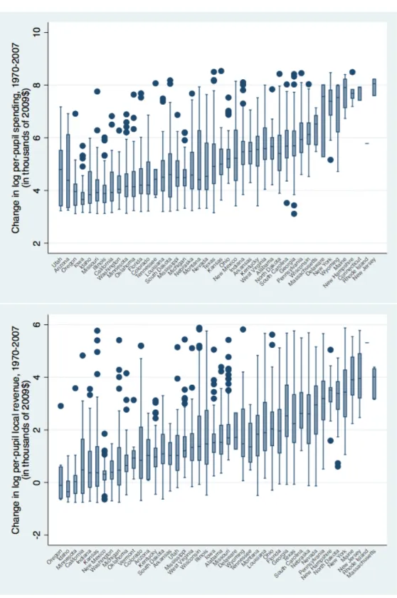
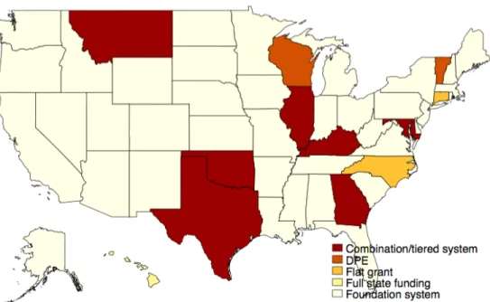
In contrast, K-12 education is the largest single element of state and local governments’ spending, about $620 billon in 2012-2013 (Figure 1), approximately 20% of their com-bined total annual budget. There is a large variation both within- and across states of the level of education spending (Figure 1.4, top panel). On one end of the distribution, Hawaii funds 100% at the state level, since it has only one statewide school district and no local districts. One the other hand, for most of the rest of the country, public education is a shared expense between these two levels of government. The extent of a school district’s authority to set budgets and raise revenue primarily depends on which education finance system is used by the state where the school district is located. The decision on how to spend the money earmarked for education, once it is collected, is also dependent on the type of funding system in use. Figure 1.5 maps the states and the funding systems they use as of 2007.

States allocate K-12 education funds to their constituent districts through funding for-mulas, which are directly related to the school finance system. There are five primary cat-egories of funding formulas currently in use, which may be used in combination by some states. These categories, in order of popularity, are the foundation system, the flat grant, local-effort equalization, equalization, and full state funding (Hightower et al. (2010)).5

The most common system of state funding, used by 38 states, is called the minimum foundation program (MFP). States under MFP guarantee a minimum spending level per student (also called foundation aid) and allow school districts to levy taxes to supplement this amount if the guaranteed level is found insufficient. The responsibility of determining the amount of foundation aid lies with state legislators and the state education agency,

5_{The analysis in this paper focuses on the experience of districts in states that use MFP. However, the}

relationship between state contributions and local contributions depend highly on the properties of the state finance system. As a result, the causal estimates presented in this paper may be different for states that do not use MFP. This is explored further in Lucasan (2018).

which may also include limits to how much additional millage (taxes) that the local school board can levy.

Local education funding levels are set by school boards under the constraints specified by state legislation. Because different states choose different tax rates and may have dif-ferent rules for the extent to which the districts can top up the state contribution, there is significant variation in the amount of public education revenues raised by local gov-ernments both across and within states. Furthermore, even within the state constraints, districts still have a lot of discretion on how much more additional taxes to raise for public education and as a result, there is also significant variation in local education revenues even within states (Figure 1.4, bottom panel).

The funding formula in use by each state can typically only be changed by a court case challenging the constitutionality of the current funding formula, or through legislation, both of which can be a difficult and drawn-out process.6 _{As a result, the funding system}

used in a state is fairly consistent, and only in very few cases is it overturned more than once each decade.7 _{Over time, the number of states using MFP has grown, and as a}

result, U.S. K-12 education finance is increasingly a top-down funding system: first states legislate the level of foundation aid, and second, the local government chooses a level of local funding in response. This dynamic decision-making process between state and local governments is the key characteristic in the model of education spending developed in this paper.

1.3

Determining per-pupil revenues at state and local levels

In this section, I develop a model that describes how state and local governments mod-ify their funding decisions in response to immigration. The basic set-up is based on the model of Fernandez and Rogerson (2003), modified to account for immigration. The pri-mary features of the model are twofold: first, state and local governments make decisions sequentially, reflecting the top-down nature of funding decisions made in states using MFP. Second, I account explicitly for immigrants having less political power than natives in mak-ing the education fundmak-ing decision at both levels of government.

The model assumes that the source of education revenues and the main avenue through

6_{Legislative changes in the funding system are more voluntary, in that the state decides whether to}

un-dergo that change. Changes due to a court case are involuntary from the state’s perspective. In the empirical work, as a robustness check I estimate all equations in a restricted sample only with states for which the last state finance reform was due to a court case. The results do not change with the restricted sample.

7_{For a list of court cases that have overturned the prevailing school finance system, see Jackson et al.}

which governments respond to immigration is a proportional income tax. The tax rate decisions are made sequentially: first, states choose a state tax rate using the median voter theorem to aggregate the constituent districts’ preferences, and once a statewide state tax rate is determined, districts choose local tax rates to supplement the state tax.

Let ts and td be the state and local district income tax rates, respectively, and educa-tion is funded through these taxes. While this is certainly a departure from the reality of property taxes funding a significant proportion of education revenues, it is a common assumption in the public goods literature. One can also think of these tax rates as taxes on an aggregate of incomes and property values; that specification would also be consistent with the model in this paper. The outcome variable corresponds to education revenues by source of funding, which in this paper is the product of tax rates and income.

I assume that there is a continuum of agents of size 1 in each district, and that are two types of agents in this economy, natives and immigrants. In order to simplify the analysis, I characterize the districts according to the average income of the natives residing in the districtyi, and also bymd, the fraction of the district population that is immigrant.

There are two goods in the economy, a consumption good c (private) and child ed-ucation q (publically provided private good). I assume that education is funded by a proportional tax on income, and all children attend local school districts. While there is a significant amount of debate in the literature about how education spending is translated to education quality, I abstract from this issue and suppose that q, the amount of child education, depends only on the amount of spending per student.

In this model, because immigrants are assumed to not vote, the utility of the district only depends on the utility of native residents, and so the private good consists of the consumption of natives only. Thus, district utility is equivalent to average native utility in the district. Later in this paper, I discuss extensions of this model where this assumption is relaxed. Consider the following utility function for a district where the average native income isyi, and has immigrant fractionmd.

U =u(ci) +v(qi) (1.1)

In (1.1), u and v are increasing inc andq, respectively, and are concave. The constraints are:

ci = (1−ts−td)yi

qi =tsy¯+tdyd

paying taxes. Child education is the lone public good, and the total amount spent on education is the sum of state and district tax revenues. The amount of educational funding raised by the state that is allocated to any individual istsy¯, wherey¯is the mean income in the state. Similarly, tdyd is the amount of educational funding raised by the local district that is allocated to any individual, whereydis the mean income in the district.

Bothy¯andydinclude immigrant income because immigrants contribute fully to the tax system and participate in public education. Mean district income can be expressed as

yd= (1−md)yi+mdym,

where yi, is mean native income, ym is immigrant mean income, and the fraction of im-migrants in district d is md. Similarly, mean state income is just the weighted average of native incomes and migrant incomes in the state.8

State legislators choose ts that applies to all districts in the state. A positive state tax rate guarantees a minimum education spending level for these districts. The mechanism that states use to determine ts is majority vote, which is characterized according to the median voter theorem. That is, the state legislators look at the preferred tax rates of all constituent districts and the median tax rate is chosen as the overall state tax rate. Because the districts decide on a local tax rate given the state’s chosen a state tax rate, the districts are able to incorporate the state’s choice in making a decision. To reflect the reality of how education funding is determined in the foundation system, I model the tax rate decisions as made at two stages: first, at the state level to determine the foundation tax rate, and second, at the local level to determine the district tax rate.

The outcome of this model will be a single t∗_s, and a value of t∗_d for each constituent district. I consider each of the two decision-making stages in turn.

1.3.1 Choosing the level of state education revenues

In this subsection, I describe the process through which a state tax rate is chosen in states with a minimum foundation tax.

The state legislator solicits preferred state tax rates from school districts, and imple-ments the median of these tax rates to be the state tax rate, in accordance with the mean

8_{Consider the following numerical example. Dexter School District, in southeast Michigan, has native}

individuals with mean income $120 (yi), and immigrants with mean income $90 (ym). Suppose that 1/3

(md) of Dexter’s population is immigrant, and so overall district income is $100 (yd). If the current state tax

rate is 20% (ts) and the district tax rate is 15% (td), then Dexter’s schools’ budget will consist of $20 from

the state of Michigan and $15 from its own residents. Furthermore, average native individual has private consumption is equal to $78, and the district’s utility isu(78) +v(35).

voter theorem. Because the median voter’s choice of state tax rate prevails at the state level, the median voter chooses state and local tax rates simultaneously. The median voter’s objective function is

max

ts≥0,td≥0u((1−ts−td)yi) +v(tsy¯+tdyd)

The first-order conditions of this maximization are:

∂U ∂ts =−yiu0 + ¯yv0 ≤0 (1.2) ∂U ∂td =−yiu0+ydv0 ≤0 (1.3)

Only one of the FOCs can be satisfied at a time. Thus, unless the median district’s income is the same as mean state income, its optimal choice will have at most one nonzero

t∗_s and t∗_d. Intuitively, the first-order conditions can be rewritten as

v0 u0 ≤ yi ¯ y (1.4) v0 u0 ≤ yi yd . (1.5)

In both equations, the expression on the left-hand side is the marginal rate of substi-tution between private consumption and education, which is the same expression in both of these equations. The expression on the right-hand side is the relative price of private consumption and education. A utility-maximizing district chooses the funding source that offers a lower relative price. This price is the tax price of education, and is defined to be the additional taxes paid by the district in order to raise spending on education by $1. State-sourced funding has tax price

tsyi

tsy¯

= yi ¯

y

while local-sourced funding has tax price

tdyi

tdyd

= yi

yd Local funding is cheaper when yi

yd

< yi

¯

y ⇐⇒ y < y¯ d, and state funding is cheaper

when yd < y¯. By relying solely on the foundation grant, poorer districts’ education are effectively subsidized by richer districts, and the chosen state tax redistributes from rich to poor. On the other hand, rich districts would prefer no redistribution, as with positive tax

rates they are subsidizing poorer districts with their taxes.

Formally, ift∗_s >0, then (1.2) implies thatyiu0 = ¯yv0, and by (1.3), −yiu0+ydv0 ≤0 ⇐⇒ −yv¯ 0 +ydv0 ≤0

⇐⇒ yd≤y.¯

Similarly, t∗_d > 0 ⇐⇒ y¯ ≤ yd. When the median district’s income is above the mean state income, it prefers to finance education purely through district collections, but if the median district’s income is below the mean state income, it prefers funding through state collections.

To characterize the median district, observe that for every district that chooses a posi-tivets, the binding FOC is given by (1.2), and preferred tax rates satisfy

yiu0((1−ts)yi) = ¯yv0(tsy¯). (1.6)

Assuming that each of the districts places one vote for their preferred state tax rate, the median voter theorem implies that the tax rate that is implemented is the tax rate preferred by the median district. As the rich districts always choose ts = 0, the state tax rate will be positive as long as the distribution of district incomes within the state is such that the median income is below the mean income. Figure 1.6 shows the districts’ state tax choices, and illustrates how the state tax is chosen from these options. The first panel shows how preferred state tax rates change with district income, yd. All districts with yd > y¯prefer

ts = 0, and all districts withyd<y¯preferts >0. Because I make no additional assumptions regarding the utility functions or the distributions of incomes, preferred ts and yd have covariance 0.

The second panel arranges the districts by preferred state tax rate, and indicates the tax rate ultimately chosen at the state level. The median tax rate, t∗_s, is positive when the median of district incomes is lower than the mean of district incomes, and t∗_s = 0 otherwise.

The effect of immigration on the state’s choice

Next, I consider what happens to districts’ preferred state tax rates and the prevailing state tax rate in the presence of immigration.

First, observe that the median voter’s preferred state tax rate is implicitly given by ymedu0((1−ts)ymed) = ¯yv0(tsy¯) ⇐⇒ ymed ¯ y = v0(t∗_sy¯) u0_((1−t∗ s)ymed) , (1.7)

where ymed is the mean native income in the median district. This expression does not depend on the level of immigration into the median district, and so the prevailing state tax ratet∗_s is unchanged by immigration into the median district.

Next, consider immigration into districts that are not the median voting district. As long as immigrants have lower income than the district mean, poor districts remain poor when immigration goes up. Poor districts’ choices of preferred state tax rates are do not depend on immigration, so that the distribution of preferred tax rates is unchanged. This implies that immigration into a poor district does not change the tax rate chosen at the state level.

On the other hand, immigration into rich districts (those for whom yd >y¯) has differ-ential effects on the district’s preferred tax rate depending on whether immigration causes district income to fall below the threshold. Suppose that immigration is low enough so that rich districts continue to be rich after increased immigration. In that case these dis-tricts continue to prefer zero tax rates, and immigration into these disdis-tricts does not affect the distribution of preferred tax rates, and the implemented state tax rate is unchanged. However, if a rich district (which by definition hasyd > y¯) receives so much immigration that its income falls below the mean state income, the districts’s preferred state tax rate increases from ts = 0 to ts > 0. This change increases the chosen state tax rate if the district’s new preferred tax rate is higher than the old state tax rate. For small changes in immigration, however, the effect of immigration into districts that are not the median district is zero.

Formally, the relationship between per-pupil state education revenues, t∗_sy¯, and immi-gration into a district,md, is given by

∂(t∗_sy¯)

∂md

= 0, (1.8)

Similarly, the relationship between the change in per-pupil state education revenues and the change in immigration into a district is given by

∂(∆t∗_sy¯)

∂∆md

= 0. (1.9)

state legislator without any consideration to district size – one district, one vote. This means that if this assumption is relaxed to allow larger districts to have more votes, if wealthier districts are larger, then the median preferred state tax rate will be lower than that predicted by the model. This is because all the wealthy districts vote for no state tax education funding, and so any estimate derived under the assumptions of this model will be a lower bound on the true impact of immigration.

1.3.2 Choosing the level of district (local) education revenues

In this subsection, I move to characterizing the local tax rates chosen at the district level, once a state tax rate has been selected.

Local districts choose local tax rates to maximize utility within the district. Consider the case when the prevailing state tax rate is positive, which occurs when the median district has income less than the mean income in the state. The district solves the following problem:

max

td≥0

u((1−t∗_s−td)yi) +v(t∗sy¯+tdyd) (1.10) Districts are allowed to increase their education spending above the foundation grant through additional taxes on district income, but are not allowed to go below the foundation grant, sotdcannot be negative. When districts opt not to top up the foundation grant, per-pupil total education spending in the district is t∗_sy¯per student. Hence the positive state tax rate guarantees a minimum education spending level for districts within the state.

The first-order condition is−yiu0((1−t∗s−td)yi) +ydv0(t∗sy¯+tdyd)≤0. Some districts are constrained by the state foundation grant to choosetd= 0. These are districts that would prefer less education, but are required by the state to provide at leastt∗_sy¯. The constrained districts are those for which

−yiu0((1−t∗s)yi) +ydv0(t∗sy¯)<0 ⇐⇒ yd yi < u 0_((1−t∗ s)yi) v0_(t∗ sy¯) . (1.11)

On the other hand, some districts will opt to top up the foundation grant, by selecting a positivet∗_d. These districts face the following first-order condition:

−yiu0((1−t∗s −td)yi) +ydv0(t∗sy¯+tdyd) = 0 ⇐⇒ yd yi = u 0_((1−t∗ s−td)yi) v0_(t∗ sy¯+tdyd) . (1.12)

The effect of immigration on the districts’ choice

Now I turn my attention to how the districts’ choice of local tax rates is affected by changes in immigration.

In the first-order conditions (1.11) and (1.12) that determine optimal district tax rates, immigration only appears in yd. Hence, the effect of immigration on a district’s choice of tax rate can be characterized based only on how md impacts yd. When immigrants are poorer than natives, more immigration results in a decrease of yd. If y0dis district income after an influx of immigrants,

y_d0 yi < yd yi < u 0_((1−t∗ s)yi) v0_(t∗ sy¯) . (1.13)

That is, constrained districts, that choose td = 0, continue to be constrained when immi-gration increases. All constrained districts choose td = 0, and so for these districts t∗d is unaffected by an increase in immigration.

For districts that are unconstrained, I can apply the implicit function theorem on the first-order condition. Hence, the effect of immigration on the district tax rate is

∂td ∂md =−(ym−yi)[v 0_+t dydv00] y2 iu00+yd2v00 . (1.14)

The sign of the relationship between the fraction of immigrants and district tax rates is the same as the sign of(ym−yi)[v0+tdydv00] = (ym−yi)[v0(q) +qv00(q)]. The expressionv0(q) +

qv00(q) is positive as long as the slopes ofv’s indifference curves in (td, q) are increasing in

yd (I will refer to this property as ISI, for increasing slopes in income, henceforth). As a proof, observe that the slope of v0s indifference curves are −yd

v0. Taking the derivative of the slope asyd changes gives the following expression:

∂slope ∂yd = v 0_[v0_+t dydv00] v02 = v0+tdydv00 v0 (1.15)

Because v is increasing, when the slope is increasing in district income, it must be that

v0+tdvdu00 >0.

Therefore the sign of ∂td

∂md

only depends on the sign ofym−yi. This implies that if im-migrants are poorer than natives, then an influx of imim-migrants lowers the district’s optimal

td, and if immigrants are wealthier than natives, then immigration increases optimaltd.9

9_{Consider the special case where the median district income in the state is higher than mean state income,}

Finally, I can characterize the effect of immigration on district education revenue, tdyd, as ∂(tdyd) ∂md =yd ∂td ∂md +td ∂yd ∂md =yd ∂td ∂md + (ym−yi)td = (ym−yi) −(yd)[v 0_+t dydv00] y2 iu00+y2dv00 +td

Again, the term in the square brackets is positive if v satisfies ISI. This implies that if, on average, immigrants earn less than natives in the district (ym −yi < 0), then more immigration leads to both a lowertdand also lower education spending at the district level. On the other hand, if immigrants earn more than natives in the district (ym−yi >0), then more immigration leads to higher education spending.

Unlike the state case, the distribution of immigrants within the state matters in the determination of t∗_d. The response of local districts to immigration depends on how im-migration affects overall district income. When immigrants are poorer than the district residents, then immigration will decreaset∗_d. Those districts that are already spending the minimum amount on education are unable to decrease education spending further, so will not change their fiscal behavior. On the other hand, when immigrants are wealthier than the district residents, an influx of immigrants increasest∗_d.

Intuitively, the previous results is because at the local level, the tax price of public education is tdyi tdyd = yi yd = yi yi+md(ym−yi) . (1.16)

Hence when immigrants are relatively poor, orym−yi <0, increased immigration increases education spending will only depend on local district tax rates. The district problem reduces to

max

td≥0

u((1−td)yi) +v(tdyd).

The first-order condition is−yiu0((1−td)yi)+ydv0(tdyd)≤0. An optimal district tax rate exists for all districts

because preferences are single peaked, and this optimal tax rate is feasible since there are no additional constraints. Applying IFT,

∂td ∂md =− ∂yd ∂md[v 0_+t dydv00] y2 iu00+yd2v00 =−(ym−yi)[v 0_+t dydv00] y2 iu00+y2dv00

This is the same first-order condition as in the t∗s > 0 case. Therefore as long as v satisfies ISI, the same

the tax price of education at the district level, as the immigrants provide a smaller fraction of tax revenues while consuming an equal amount of education. Similarly, when immi-grants are relatively wealthy, more immigration decreases the tax price of education for natives at the district level, as the new immigrants provide more taxes relative to increased education costs. However, this mechanism works only at the district level.

1.3.3 Summary of model predictions

In the previous subsection, I developed a model of education finance that allows me to make predictions on how immigration influences the amount of money raised to finance public education.

The first implication of the model is that per-pupil state education revenues are inde-pendent of immigration after controlling for average income within a state. This is because for the median district, an additional dollar of education spending costs yi/y¯. As long as native income in the median district is less than the state average income, the state tax rate will be positive. Furthermore, immigration only affects the tax price of education for the median district through its effect on state mean income. Hence, I have the following empirical prediction: within a state, state education contributions allocated to a particular district is independent of immigration into said district

The second implication of the model is that at the district level, per-pupil district rev-enues are affected by immigration through the district mean tax rates. When deciding to raise education revenues locally, an additional dollar of education spending costs yi/yd. When immigrants are relatively poor, more immigration decreases yd relative to yi, and the tax price of education spending is higher in those districts. This leads to less edu-cation spending in districts with more immigration.For an illustrative example, consider two districts where one has more immigrants than the other. Under the assumption that immigrants are the same everywhere, in order for these districts to have the same average income, it must be that district with the higher percentage of immigrants also has wealth-ier natives.10 _{Then the tax price of education,y}

i/yd, is higher in the district with more immigrants. If these districts get the same change in immigrant share, if the district with wealthier natives will end up with lower district income, and the tax price of education will

10_{To see that this is true, note that since the average district incomes are the same,}

yd=yd0 ⇐⇒ (1−m_d)y_i+m_dy_m= (1−m_d0)y_i0+m_d0y_m

(1 +md0)(y_i−y_i0) = (m_d−m_d0)(y_i−y_m).

Because immigrants have on average lower incomes than natives, the term on the right-hand side has the same sign as(md−md0). Therefore, when a district has more immigrants,m_d> m_d0, then it must also have

further increase. The model predicts that the district with wealthier natives will choose to spend less on education in response to immigration.

Finally, in any school district, total education spending is t∗_sy¯+t∗_dyd. The impact of immigration on total tax revenues should broadly follow the direction of the impact on the district tax rates, but should be smaller in percentage terms due to the district response being diluted by the inaction of the state government.

A summary of model predictions is available in Table 1.1. In succeeding sections, I test this set of predictions on U.S. data. I will first describe the data that I use and the empirical equations, followed by an analysis of the main results.

1.4

Data

I test the implications of the model presented in the previous slide by applying it to a unique panel dataset covering the period 1970-2007. The primary data sources are the National Center for Education Statistics Local Education Agency Financial Surveys (F-33) for school district spending data and tabulations from the decennial Censuses for demographic data. For non-decennial years, I use the American Community Survey 2005-2007 3-year estimates. The NCES data collects data from the population of school districts only in years that end in 2 or 7. Hence the 1970, 1980, 1990, and 2000 SD financial data are from the surveys collected in 1972, 1982, 1992, and 2002 respectively. The 2007 financial data is from the 2007 wave of the NCES survey.

School district boundaries can change year to year, and in constructing a panel cover-ing a long time period, it is very important to keep the school districts consistently defined over time. In order to do so, I use the 1969-1970 Geographic Reference File to assign con-temporary school districts to the county they would have belonged to in 1970, resulting in a panel of observations at the county level. In cases where a school district belonged to more than one county, I assign its data to the parent counties according to population weight. For example, if the Ann Arbor school district had 80% of its population in Washt-enaw county and 20% in Wayne county in 1970, then in subsequent years, I will always assign Ann Arbor’s information to Washtenaw and Wayne counties in those proportions.

Constructing the panel at the county level has other advantages. First, counties are consistently defined over a long period of time, certainly longer than school districts. Sec-ond, school districts vary in the grades of schooling they offer, and some grade levels are more expensive to offer than others. By aggregating up to the level of the county, these concerns are minimized. This approach also ensures that the two-year gap between the financial data collection and the decennial Census does not cause inconsistencies, since all

the data is transformed into its equivalent 1970 county.

School districts can be broadly categorized as fiscally dependent or independent. De-pendent school districts are those with no responsibility for fiscal decisions. Another gov-ernment entity, often the local state, city, county, or municipal govgov-ernment, will approve the budget and set appropriate tax rates to support these budgets in dependent school districts. The vast majority of school districts, however, are fiscally independent, where the local school boards have the authority to develop a district budget and set tax rates in order to support their chosen budgets. The analysis is limited to independent school dis-tricts, which are able to select their own budgets and set tax rates without going through an external government entity.

In Hawaii, Maryland, North Carolina, and the District of Columbia, there are no inde-pendent school districts. Hawaii and the District of Columbia both have just one school district. Maryland and North Carolina both only have school districts that are run at the county level. The remaining states generally have a combination of both dependent and independent school districts.

My analysis also only includes states that use the minimum foundation system (as well as states that use MFP in combination with another financial system), as the theoretical model assumes a two-stage state and local decision that only occurs under MFP. While increasing numbers of states use MFP, not all of them consistently use MFP throughout the sample period. For some states, Supreme Court cases have reformed the existing state finance system, and the primary state education finance system may change in between time periods. I include a state x year observation in my sample as long as at the time the financial data was collected, the state was under an MFP system. The data on court cases is derived from Jackson, Johnson, and Persico [2014]. The full sample consists of 7,251 county-year observations between 1970 and 2007.

1.5

Empirical framework

In this section, I describe the equations I use to estimate the impact of immigration on education spending, and analyze the findings at both state and local levels. The goal here is to disentangle the separate responses of state and local governments to changing tax prices induced by immigration. First, note that the model implications described in the previous section are based on three parameters: the fraction of immigrant population,md; average district income,yd; and, for the district-level analysis, prevailing state tax rates t∗s.

The general form of the estimation equation is

lnYc,t=β0+β1Immc,t+β2Incc,t+Xc,t0 δ+λstate+γt+c,t (1.17) where the outcome variable, lnYc,t, is the logarithm of one of several fiscal per-student variables in local county c. In the first set of results, lnYc,t is the log of current spend-ing per student. This variable excludes not just capital outlays and current outlays but also transfers to private schools and charter schools, and is most comparable to existing analyses that only look at current spending. In the next set of results, lnYc,t is the log of state education revenues per pupil and local education revenues per pupil. The primary explanatory variable, Immc,t, is the proportion of foreign-born residents in local county

c at time t. I control for a set of various time-varying county characteristics, including a proxy for education demand, the relative size of elderly and school-age populations, and log median income within the county. I also include state- and time- fixed effects. I cluster the standard errors at the county level.

Because the local county’s decision depends on the amount of state education contri-butions, the estimation equation for local revenue estimation is

lnYc,t=β0+β1Immc,t+β2Incc,t+β3StateRevc,t+Xc,t0 δ+λstate+γt+c,t (1.18) whereStateRevc,t is the amount of state contributions to public education in the county. 1.5.1 First-differenced estimates

Using changes in the fraction of foreign-born as an explanatory variable provides sev-eral advantages over using levels of the fraction foreign-born. First, I am able to eliminate bias due to time-invariant characteristics. Second, to the extent that immigration patterns have changed over time, I am able to utilize increased variation in the immigrants’ location decisions across time to estimate β1. In particular, consider that the state with the largest

increase in the share of population that is foreign-born is different in 1970 than it is in 2007.

I focus on long differences for two reasons: First, the one-year change in the fraction of foreign-born population, my primary explanatory variable, is very small and exhibits considerable noise. In addition, I am concerned about mean reversion in the fraction of foreign-born population11. Looking at a longer difference allows a more accurate measure

11_{To think about mean reversion in the context of the foreign-born population, consider the following}

example. Suppose that the number of immigrants entering Washtenaw county follows a fixed distribution. In yeart−1, Washtenaw receives more immigrants than average. Since the distribution of immigrants is

of the changes in foreign-born population. I perform my analysis using the decennial years 1970, 1980, 1990, 2000, and 200712_.

I estimate the first-differenced equation version of (1.17),

∆ lnYc,t =β1∆Immc,t+β2∆Incc,t+ ∆Xc,t0 δ+γt+εc,t (1.19)

WhenYc,tis state revenues per pupil, β1 corresponds to a linear approximation of ∂t∗_sy¯

∂md . When Yc,t is local revenues per pupil, the estimation equation is the first-differenced version of (1.3),

∆ lnYc,t=β1∆Immc,t+β2∆Incc,t+β3∆StateRevc,t+ ∆Xc,t0 δ+γt+εc,t (1.20)

The coefficientβ1 corresponds to a linear approximation of ∂t∗_dyd

∂md .

1.5.2 IV estimation

A limitation of OLS or first-differences models when analyzing the impact of immigra-tion on educaimmigra-tion spending is the possibility that the endogeneity of migrants’ locaimmigra-tion decisions may lead to biased estimates. As suggested by Tiebout (1956), and several subsequent papers (Goldstein and Pauly (1981), Rubinfield et al. (1987), among others), families may sort into counties according to their preferred level of public good spending, and this residential sorting would distort the causal effect of immigration of education rev-enues. In particular, because public education benefits accrue primarily towards younger households and households with children, counties that spend more on public education may attract more immigrants. We might see that immigrants, who skew younger and may have children that directly benefit from public education, select into areas with high edu-cation spending. Alternatively, immigrants may prefer to move to areas with good labor market conditions, or to areas that are more immigrant-friendly. The potential endogene-ity of immigrant location decisions is corroborated by Figure 1.7, which shows that the wealthiest counties have the fastest growing immigrant populations. To the extent that wealth is a proxy for the good labor market conditions that attract immigration, one may observe that counties with more immigration also spend more on education, but this could constant, implies that in year t, Washtenaw is more likely to receive fewer immigrants compared to the previous year. Mean reversion implies that∆Immc,t =Immc,t−Immc,t−1is lower, and leads to positive

bias in theβ1estimate.

12_{I use 2007 instead of 2010 to avoid confounding effects due to the Great Recession. As for the possibility}

that the Great Recession may have impacted education finance prior to 2007, I present robustness checks of all my estimates excluding 2007 from the analysis in a later section.

just be the result of selection bias and not a truly causal effect.

An instrumental variable strategy is required to eliminate the bias caused by endo-geneity and consistently estimate the effect of immigration of education spending. My preferred instrument uses historical migration patterns to predict where new immigrants choose to locate, similar to approaches taken in the immigration literature (Card (2001), Wozniak and Murray (2012)). New immigrants tend to be concentrated geographically and come to the same areas where earlier immigrants from the same source country have chosen to reside (Bartel (1989)). That is, I employ an instrumental variable technique that uses historical immigration settlement patterns to predict current migration patterns. This instrument is particularly attractive because I avoid the possibility of endogenous sorting among immigrants. It stands to reason that 1970 immigrant settlement patterns will not affect contemporaneous choices of education spending outside of its impact on current migration. To be precise, I construct the following:

ˆ Mc,t= Nc,1970 Ns,1970 Mc,t (1.21) IV = Nc,t−1+ ˆMc,t Tc,t−1+ ˆMc,t − Nc,t−1 Tc,t−1 (1.22)

In (1.21),Ms,t is the number of people residing in stateswhose reported year of entry into the U.S. is between t−1 and t. The variable Nc,1970 is the number of foreign-born

residents that live in countycin 1970, whileNs,1970 is the number of foreign-born residents

in the entire state s in 1970. Hence Nc,1970

Ns,1970

is the fraction of all foreign-born in the state that lived in the county. The variable Mˆc,t is an approximation of how many of the new foreign-born that moved into the state moved intoc.

Next, in (1.22), Tc,t−1 is the total number of residents of countycat timet−1, so that Nc,t−1

Tc,t−1

is the actual fraction of countyc’s population that was foreign-born at timet−1. The term Nc,t−1+ ˆMc,t

Tc,t−1+ ˆMc,t

is an approximation of the fraction foreign-born int. The instrument, denoted IV, is an approximation of the change in the fraction of foreign-born population betweent−1andt.13

13_{Consider the following numerical example. In 1970, Washtenaw had 10 foreign-born residents, out of}

the Michigan total of 100. Thus Nc,1970 = 10and Ns,1970 = 100. If Michigan received 2000 new

immi-grants between 1990 and 2000, then the approximate number of new immiimmi-grants coming to Washtenaw is (10/100)(2000) = 200. If in 1990 Washtenaw had 500 foreign-born residents and 1000 native-born residents,

1.6

Results and Analysis

In this section, I present the result from the estimation framework described in the previous section. I first analyze this data set graphically to observe if the patterns in levels data are consistent with the model presented in the previous section. I then test whether the instrumental variable I use is credible by checking that the identification assumptions are satisfied. Then, I move on to formal analysis of the estimation findings.

1.6.1 Graphical analysis

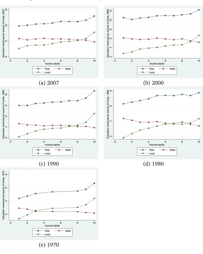
I explore whether the predicted pattern between mean income and total spending is apparent in the data even without controlling for any covariates. I categorize counties into deciles according to their mean income. In Figure 1.8, I graph local, state, and total education revenues against these deciles. What is apparent is that per-pupil state revenues are decreasing income, and per-pupil local revenues are increasing with median income. As local revenues increase more than the decrease in state revenues, overall education revenue increases with income. The graph also shows that over the panel time period, state contributions are higher than county contributions in relatively poorer counties, and only for the top 2-3 deciles is the county contribution higher than state contributions.

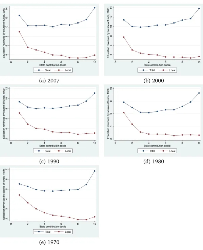
Finally, I look at the relationship between state revenues and local revenues. Similarly to the previous graph, I sort counties into deciles according to per-pupil state contributions to education. I then graph how county revenues and total revenues14 _{evolve across these}

deciles. Table 1.9 shows that as per-pupil state revenues increase, county contributions fall before leveling off. This is consistent with the model prediction on county tax revenue: the higher state taxes are, the more counties are constrained to choosing not to top up the foundation grant. Hence, for high state contributions the county contributions level off and become flat. Furthermore, at low levels of state contributions, average local revenues are higher because fewer counties are constrained. Finally, total spending is U-shaped relative to state revenues, so that the counties that receive the lowest and highest amounts of state aid have relatively high total education revenues per pupil.

the instrument will be equal to

IV = Nc,t−1+ ˆ Mc,t Tc,t−1+Mˆc,t −Nc,t−1 Tc,t−1 = 500 + 200 1500 + 200− 500 1500= 0.078.

1.6.2 Testing the credibility of the instrumental variable approach

The identification strategy requires two assumptions: that the instrument is correlated with actual changes in the fraction of foreign-born population, and that it is uncorrelated with the other factors that affect per-pupil state and local education revenues.

I provide evidence for these assumptions. Table 1.4 contains an estimate of the first-stage relationship between the instrument and the change in fraction of foreign-born pop-ulation in each state for the baseline specification for estimating state revenues. It also contains the first-stage estimate where ∆StateRevc,t is added as a regressor, which is the specification used to estimate the local revenue equation. The F-statistics in both spec-ifications are similar, 25.96 and 25.81 respectively15_{. This indicates a strong first-stage}

relationship and is evidence that the first assumption is satisfied.

Next, I investigate support for the exogeneity assumption required for IV estimation. Table 1.5 has estimates of the relationship between the pre-existing trend in per-pupil state and local revenues from 1965 -197016 _{and the instrument. If the instrument is able}

to predict the pre-existing trend, then the instrument is very likely to fail the exogene-ity assumption. I find that the coefficient estimate of this relationship is not statistically significant. To address concerns about the extent to which this finding may be due to confounding effects of traditional immigrant settlement states, I rerun these regressions while excluding Texas and California. I find that excluding Texas and California reduces the coefficient estimate of the effect of immigration on this pre-existing trend. However, I find no significant impact. Thus, these tests indicate that the instrument is not driven by these immigrant states.

1.6.3 Estimation results

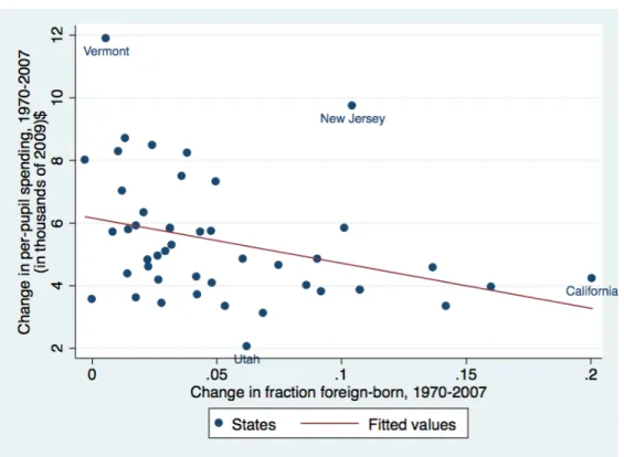
I now turn to analysis of the estimation results. The OLS levels estimates do not follow the same pattern described in the model. Instead, it shows that state education revenues are lower and local education revenues are higher in counties that experience the most immigration (Tables 1.2 and 1.3, respectively). However, in Figures 1.10, 1.11, and 1.12, I construct scatterplots of state-level changes in immigration over the time period 1970-2000 and the corresponding change in per-pupil fiscal variables. Figure 1.10 shows the correlation between the change in the fraction of foreign-born population and the change in per-pupil current spending between 1970 to 2007. I construct state-level observations

15_{The similarity of these F-statistics is as expected. The only difference in these first-stage regressions is}

the addition of a single covariate,∆StateRevc,t.

16_{Due to the timing of the Local Finance Surveys, this variable is actually the change in per-pupil revenues}

by taking the mean of these variables across all counties in each state, weighted by the county population in 2007. I then draw a scatterplot of these variables. I observe that states that have higher increases in the fraction of foreign-born population have lower increases in per-pupil current spending. Figure 1.11 is similar to Figure 1.10, but with shorter 10-year differences, to illustrate that this negative relationship is also visible with shorter time horizons. Figure 1.11 contains the corresponding scatterplots for the changes between the following years: 2000-2007 (Panel a.), 1990-2000 (Panel b.), 1980-1990 (Panel c.), and 1970-1980 (Panel d.). I observe that the negative correlation observed with current spending between 1970-2007 is also apparent when looking at these shorter ten-year differences. These general trends mirror the predictions of the model presented in the previous section. Figure 1.12 shows the correlation between changes in the frac-tion of foreign-born populafrac-tion and per-pupil state revenue (Panel a.) and per-pupil local (county) revenue (Panel b.). The same pattern is evident: States with higher increases in the fraction of foreign-born population have lower increases in both per-pupil state revenues and per-pupil local revenues.

These estimates and scatterplots suggest that per-pupil current spending and per-pupil local revenues rose less in states that saw the largest growth in the fraction of immigrants. This also suggests that the correct estimation strategy should focus on changes, not levels. In other words, running first-differenced regressions will give a more accurate estimate of how education responds to immigration.

Tables 1.6 and 1.7 present the first-difference OLS and 2SLS estimates of the effect of a rising fraction of foreign-born population on state-sourced and locally-sourced K-12 education revenues. The first coefficient estimate presented corresponds to β1, the

coeffi-cient on the primary explanatory variable, which is the change in the fraction-foreign born residing in the county. The second coefficient estimate presented, β2, is the coefficient

on changes in median family income. Standard errors, which are presented below the coefficient estimates in parentheses, are clustered at the county level.

The first four columns of Table 1.6 present the first-differenced OLS results for the state revenue equation. I find that per-pupil state education revenues are negatively associated with education spending. Furthermore, accounting for county-level controls on the age distribution and demand for education does not eliminate this association. However, the magnitude of the estimate decreases as I add more regressors, which indicates a potential relationship between the change in fraction-foreign born and county characteristics.

The remaining columns of Table 1.6 contain the instrumental variable results. The IV estimates are not significant, which are in line with the model predictions presented earlier. In column (6), I control for the change in the fraction of college-educated residents,

which is a proxy for the county’s preference for education. Adding this regressor decreases the magnitude of the IV estimate, but the estimate on fraction college-educated is not statistically significant. In column (6), I add controls for the age distribution of residents in the county. The coefficient on the fraction of population that is under age 18 is significant and negative, but this is likely due to the high correlation between this variable and the number of students enrolled in the county, and is just a mechanical relationship. The coefficient for the fraction of population that is above age 65 is negative, consistent with the elderly voting in their own self-interest (Ladd and Murray (2001)), but the estimate is not statistically significant.

The coefficient for median income is negative and statistically significant for the first three IV specifications (Columns (5), (6), and (7)), which is consistent with the predictions of the model. However, controlling for the poverty rate (Column (8)) causes the coeffi-cient on median income to become insignificant. This indicates that counties with more poverty receive higher state contributions to education. This indicates that poverty rates and median income perform similar roles for determining state contributions to education within a county.

Although they are insignificant, the IV estimates for the effect of a change in the fraction foreign-born population are more negative compared to the equivalent OLS estimates. This is as predicted – the OLS estimates do not account for the fact that immigrants may sort into counties according