Banco de M´
exico
Documentos de Investigaci´
on
Banco de M´
exico
Working Papers
N
◦2008-13
Transparency and Numeric Rules in the Budgeting
Process: Theory and Evidence
Nicol´
as Amoroso
Banco de M´exico
September 2008
La serie de Documentos de Investigaci´on del Banco de M´exico divulga resultados preliminares de trabajos de investigaci´on econ´omica realizados en el Banco de M´exico con la finalidad de propiciar el intercambio y debate de ideas. El contenido de los Documentos de Investigaci´on, as´ı como las conclusiones que de ellos se derivan, son responsabilidad exclusiva de los autores y no reflejan necesariamente las del Banco de M´exico.
The Working Papers series of Banco de M´exico disseminates preliminary results of economic research conducted at Banco de M´exico in order to promote the exchange and debate of ideas. The views and conclusions presented in the Working Papers are exclusively the responsibility of the authors and do not necessarily reflect those of Banco de M´exico.
Documento de Investigaci´on Working Paper
2008-13 2008-13
Transparency and Numeric Rules in the Budgeting
Process: Theory and Evidence
*Nicol´as Amoroso†
Banco de M´exico
Abstract
In this paper I develop a simple dynamic agency model postulating that, among bud-getary institutions, transparency of the budgeting process is the main driving force in ex-plaining differences in fiscal outcomes and that budgetary numeric rules can be an active long-run constraint only if the budgeting process is transparent enough. The model does not only account for long-run differences where countries with better budgetary institutions will have more disciplined fiscal outcomes, but can rationalize situations where countries with relatively better budgetary institutions can have what would appear to be less disciplined fiscal outcomes in the short-run. Empirical tests corroborate some but not all of the model’s predictions.
Keywords: Budgetary Institutions, Fiscal Outcomes, Transparency.
JEL Classification: H61, D70, E60.
Resumen
En este art´ıculo se presenta un modelo de agencia din´amico en el cual se postula que la transparencia del proceso presupuestario es la principal causante de las diferencias en los resultados fiscales, y que las reglas num´ericas sobre el presupuesto pueden ser una restricci´on activa en el largo plazo, ´unicamente si el proceso presupuestario es lo suficientemente trans-parente. El modelo puede explicar no solo diferencias en resultados fiscales en el largo plazo, d´onde pa´ıses con mejores instituciones siempre tendr´an resultados fiscales m´as disciplina-dos, sino tambi´en racionalizar situaciones de corto plazo, donde pa´ıses con relativamente mejores instituciones presupuestarias pueden presentar resultados fiscales que en aparien-cia son menos disciplinados. Los resultados emp´ıricos del trabajo corroboran algunas de las predicciones del modelo.
Palabras Clave: Instituciones Presupuestarias, Resultados Fiscales, Transparencia.
*This paper has benefited from the comments of Carlos Capistr´an, Daniel Chiquiar, Allan Drazen, Wallace Oates, John Wallis and participants of the International and Domestic Macroeconomics seminars at the University of Maryland and the research seminar at Banco de M´exico.
1
Introduction
“Elected officials typically enjoy an immense informational advantage over the voters that limits how accountable such agents will be to the voters desires. This is a consequence of the complexity of modern government.” (Ferejohn (1999)).
Budgetary Institutions are defined as the set of all the rules and regulations according to which budgets are prepared, approved and carried out (Alesina and Perotti (1999)). What is the role of budgetary institutions in shaping the size of the budget and, ultimately, the delivery of public goods? How independent are these institutions from each other and which ones, if any, are truly necessary to affect fiscal outcomes? This paper deals with these questions and explains how different countries that are supposed to obey the same set of rules, such as the members of the European Union and the Maastrich Treaty, can have dissimilar fiscal outcomes. In other words, it will provide an explanation of how and when these rules will be an active constraint on the government.
In this literature, stronger fiscal institutions are defined as those that provide more dis-cipline in the budgeting process, reducing the margin for unproductive spending (Poterba and von Hagen (1999)). The implication is that, other things being equal, stronger in-stitutions should cause, by means of stricter constraints, lower deficits and levels of debt for the same amount of public goods. The budgetary institutions that are analyzed in the present paper are the transparency of the budgetary process and the set of numeric rules imposed on the budget. Transparency of the budgetary process can be defined as the degree of openness towards the public at large about government structure and functions, fiscal policy intentions, public sector accounts, and projections (Kopits and Craig (1998)). Numeric rules imposed on the budget can take the form of specific limits to expenditures, debt and deficit, or restrictions to the flow of resources between and within programs, agencies and levels of government. These constraints could even be restrictions to the flow of resources between different fiscal periods.
To study these two budgetary institutions, in the first part of the paper I provide a career concern model in which the government has an agency relationship with their constituents and might enjoy some information advantages, depending on the degree of transparency of the budgetary process. Voters can try to discipline the incumbent through elections and by imposing numeric rules. The results of the model show that more trans-parency will increase fiscal discipline, while numeric budgetary rules will be effective only if the budgetary process is transparent enough.
This model was inspired by two well known pieces in the political economy literature: the political business cycle model with prospective voting (Rogoff and Siebert (1988), Ro-goff (1990), Shi and Svensson (2001)), and the elections as a disciplining device model with retrospective voting (Ferejohn (1986)). To the best of my knowledge, no other
work –besides Milesi-Ferretti (2004)– provides a theoretical framework for the relation-ship between transparency and numeric constraints on the budgeting process and their implications over deficits or other fiscal variables. The novel characteristics of the model presented here are: First, the model is able to accommodate not only long-run results, where stronger institutions will always cause more constrained fiscal outcomes, but also short-run implications, where countries with relatively stronger institutions can be paired with relatively unconstrained outcomes. Second, the main claim of the model is that transparency is the major force for generating differences in the levels of debt, and that numeric constraints can have opposing effects for the same numeric rule, depending on the level of transparency.
The second part of the paper provides empirical evidence of the effects of budgetary institutions on fiscal outcomes. I exploit a new data set to construct measures of numerical constraints on the budget and the degree of budgetary transparency, and assess their influence on a series of fiscal outcomes. In particular, I test the two principal implications of the theoretical model: (i), that more transparency will increase fiscal discipline and,(ii), that numeric rules will increase fiscal discipline only if the budgetary process is transparent enough. The results of the regression analysis indicate that the only budgetary institution that appears to have an effect on fiscal outcomes is the transparency of the budgetary process. I do not find, however, an effect of numeric rules on fiscal outcomes conditional on the level of transparency.
The rest of the paper is organized as follows: In section 2 I review the literature. Section 3 presents the career concern model. Section 4 shows the empirical evidence and section 5 concludes.
2
Literature Review
The theoretical model presented in this work is related to the following literature. Shi and Svenson (2001) propose a moral hazard model of electoral competition to explain a set of empirical findings about thesize of electoral budget cycles, and conclude that these depend on the rents of those remaining in power and theshare of informed voters. Alt and Lassen (2003) slightly modify the Shi and Svenson model and reinterpret the share of informed voters as transparency in the budgeting process, and conclude that lower transparency produces higher levels of debt and larger deficits. The problem with these models is that in the absence of electoral cycles (i.e., if there were no elections or if elections occurred in every period), no debt or deficit could be generated. In other words, the Alt and Lassen model predicts that transparency affects fiscal outcomes only in the electoral year. In contrast, the model presented here builds on some of the structure of the Shi and Svenson model, but eliminates the political fiscal cycle motive by allowing elections to occur in every period. In spite of this change, the current model still generates an inverse relationship
between transparency and debt. This is relevant not only from a conceptual perspective, but also because the majority of empirical tests (Alesina et. al. (1998), Alt and Lassen (2003)) analyze the cross-sectional implications of transparency in fiscal outcomes and none of them show evidence that an election dummy is significant.
In a seminal paper, Ferejohn (1986), obtained optimal reelection rules when the incum-bent’s actions cannot be directly observed by retrospectively inferring these actions based on realized outcomes. This pure outcome evaluation can be interpreted in the context of the model presented here as a case of full opacity, where the signal drawn by the electorate is simply uninformative. Persson, Roland and Tabellini (1997) (PR&T), in a similar setup, also derive the case of full information, where voters can observe incumbent’s actions, and show that even in this case the incumbent will extract rents from being in power. In terms of the present model this could be associated with a case of full transparency where the signal drawn from the private sector perfectly identifies the current shock. Whereas the structure for obtaining the optimal reelection rule is similar to these two previous works, there are some differences that are worth mentioning. Here, the state of the world is not only determined by an exogenous shock, but also by the history of policy decisions made by the incumbent. This feature allows situations where the incumbent will optimally choose to perform actions that are costly only to him and be reelected, even under the most adverse of shock realizations, provided he has enough fiscal resources, i.e. that issuing new debt is not too costly. A second difference between this model and those mentioned previously lies in the fact that I analyzed different degrees of informational asymmetry, and their relation to fiscal outcomes in addition to welfare.
The work that is most closely related to the model presented here is Milesi-Ferretti (2004) which is the first, and to the best of my knowledge, the only paper that looks at the effects of budgetary rules and budgetary transparency simultaneously on fiscal outcomes. In a two-period model, with heterogenous policymakers that seek to minimize an arbitrary loss function, Milesi-Ferretti shows that the extent to which a myopic ruler will engage in creative accounting (defined as deviations from a preestablished budgetary rule) depends negatively on the transparency of the budgetary process. There are two key differences between the two models. The first one is conceptual. The mechanics of Milesi-Feretti’s model requires a numeric rule to be imposed in order to generate differences in fiscal outcomes. In other words, the same policymaker, if not faced with a numeric rule on the budget, will deliver the same fiscal outcome under two different transparency regimes. By the contrary, the model presented here postulates that policymakers facing different transparency regimes will deliver different fiscal outcomes even without the imposition of a numeric rule. The second important difference is that Milesi-Ferretti’s model can only account or be interpreted for long-run results whereas my model also rationalizes short-run outcomes, as was already mentioned.
Several papers have empirically explored the question of whether budgetary institu-tions matter. In a series of papers, von Hagen (1992) and von Hagen and Harden (1994)
and (1996), study the effects of budgetary institutions as a whole. They combine in a single index elements that corresponds to transparency as well as to the voting procedure to pass the budget, classified in a hierarchical-collegiate spectrum. They find that more hierarchical and transparent budgetary institutions are associated with more fiscal disci-pline. Exploring further, von Hagen (1992) suggests that transparency comes second to hierarchical features in order of importance. De Haan et. al. (1999) use new informa-tion available to update von Hagen’s index for an almost identical sample. These authors corroborate von Hagen’s result that better budgetary institutions as a whole induce fiscal discipline. However, they conclude that although the results are statistically significant, these are not economically important as was previously claimed.
Alesina et. al. (1999) pursue a different strategy by constructing separate measures for every category of the budgeting process for a sample of twenty Latin American countries. Employing fiscal deficits as their fiscal outcome measure, these authors arrive at the con-clusion that fiscal procedures matter for fiscal deficits among Latin American countries, but when they look at the disaggregated indexes, they find that numerical rules and hi-erarchical procedures matter but transparency does not. They do acknowledge, however, that the “results on transparency probably say more about the difficulty of measuring it, than about its effect on fiscal discipline” (Alesina and Perotti (1996) p.405). Filc and Scartascini (2004), employing a new data set that allows them to measure budgetary insti-tutions ten years later, closely follow Alesina et. al. (1999), and perform the same exercise for a sample of eleven Latin American countries arriving, at the same conclusions.
Alt and Lassen (2003), using data from 19 OECD countries, concentrate exclusively on the effects of fiscal transparency on public debt and the central government expenditure. These authors make a successful attempt at providing guidance about what should contain a good measure of transparency. They find significant and economically important effects of transparency, especially for public debt.
3
A Career Concern Model
I consider an economy populated by a continuum of mass one of identical and infinitely lived individuals called voters. At every moment in time an incumbent, picked randomly from within the economy, is in charge of the government and will remain in power until he is voted out and replaced by an identical agent, who was a voter at the end of the last period, and who now becomes the new incumbent. The former incumbent returns to the population as a voter, and while nothing forbids him from being elected again, the probability of this event happening has measure zero.
Utv =gt, (1)
where g represents per capita amounts of the public good. What is important to note about equation (1) is that voters know exactly how much of the public good they are consuming in each period.
The incumbent’s period utility function is identical to that of voters, since the in-cumbent rose from within the population, but incorporates costs and benefits of being in office:
UtI =gt+χ−φ(et), (2)
where χ represents ego rents from being in office, charged every period t, and φ is the disutility function of the effort variable, et, which is the amount of effort measured in
dollars that the incumbent devotes to public good production in the present period, and that is unobserved by voters. I assume that φ is twice continuously differentiable and strictly convex, which implies that the extra unit of effort is ever costlier. Both the incumbent and voters are assumed to maximize expected utility.
The production of the public good is described by the following equation:
gt=θt[dt+et]−D(dt−1), (3)
where dt is the per period government new debt maturing in the following period, and
D(dt−1) is the amount of debt plus interest payments maturing this period. Whereas d
and e are choice variables for the government, θt represents an exogenous shock to the
production of public goods. It can be thought of as an input shock summarizing the cost and composition of raw materials in the production of public goods. I assume that the set of possible values that θ can take is continuous, compact, time invariant, and common knowledge for voters and incumbent alike: everyone knows thatθt∈[θ, θ]. I further assume
that θ is identically independent distributed (iid) over the mentioned set with E(θ) = 1. With respect to the cost of public debt, I follow the same assumptions as Shi and Svensson (2001) or Alt and Lassen (2003), where D(d) is defined as a convex borrowing function. In particular,D(0) = 0,D0(0) = 1, andD00(d)>0 for alld >0. The convexity of
Dmeans that the marginal cost of borrowing is increasing in the amount of the principal, which can be linked to the country risk premium.
3.1
Transparency in the Budgeting Process
Transparency of the budgetary process is understood along the lines of Kopits and Craig (1998), who define transparency as openness towards the public at large about government structure and functions, fiscal policy intentions, public sector accounts, and projections.
Transparency involves ready access to reliable, comprehensive, timely, understandable, and internationally comparable information on government activities, so that the electorate and financial markets can accurately assess the government’s financial position and the true cost and benefits of government activities, including their present and future economic and social implications.
Clearly, there is the question if transparency is always beneficial. As it has been argued (Prat, 2005), too much transparency on the agent’s actions can lead to outcomes that are detrimental for the principal. In the context of the present paper, one could think of too much transparency generating a situation of sclerosis in policy implementation, perhaps due to conflict of interests between agents. This paper abstracts from this situation and it can be interpreted as looking only into the segment where more transparency always increases government efficiency.
Here, I condense this notion of transparency in the budgeting process as the ability of voters to observe the true costs and composition of inputs involved in the production of the public good. That is, the potential to assess the true value of θ. In this respect, I assume that only the incumbent can directly observe θ. On the other hand, voters obtain anestimate1, ˜θ, of the true value of the shock, conditional on the degree of transparency
and the actual realization of θ. For each level of g, the government will like voters to believe that θ was lower than the actual value and, consequently, make e appear to have been higher than the level exerted.
Some real world examples that help us understand this mechanism would be:
• Price of cement, steel, aluminum, etc: Voters can see new infrastructure but they can’t know for sure what materials were used to build it. More importantly, without periodical revisions of the expending accounts, expenses at the end of the year can be justified claiming the material was purchased at the peak of the price within the year.
• Detail over contractors (suppliers): if payments to contractors are fully aggregated (low transparency), then it is easy to overstate costs. If on the contrary they are more disaggregated, this possibility is reduced.
To incorporate this idea in the model, I consider the degree of transparency of the budgetary process to be inversely related to a measure²∈[0, ²], that is, more transparent regimes are associated with a lower value of ². I treat ² as a parameter that is both exogenous and known to the incumbent and voters alike. The reason is that I am interested in the effect of transparency over fiscal outcomes rather than on the dynamic properties of transparency itself which, although a very interesting question, goes beyond the scope of
this work. I then assume voters will draw a ˜θ that depends on the given exogenous value of ², the unobserved realization of θ, and its distribution f(θ). I treat ˜θ as a continuous uniform random variable that can take any value over the moving interval [max(θ, θt −
²),min(θ, θt+²)].
The inference process about the true value of the shock is informative if it helps to further bound the set of possible θ. Depending on the level of transparency there are four possible information regions:
1. Full Transparency (² = 0): in this case ˜θ = θ. This is the most informative case, where the signal is the shock.
2. High Transparency (²≤ θ−θ2 ): in this case the inference process is always informative in the sense that the signal will give a range of the true value of the shock that is a subset of [θ, θ]: ˜θ ⇒θ∈[max(˜θ−², θ),min(˜θ+², θ)].
3. Low Transparency (θ−θ2 < ² < θ−θ): in this range, depending on the realization of ˜
θ, voters might not be able to reduce the set of possible realizations of θ.
4. Full Opacity (² ≥ θ−θ): a case in which the inference process is simply not infor-mative.
Given the voter’s inference process and ² > 0, the conditional expectation of θ on the estimated shock will be:2
E(θ|θ, ²˜ ) =
Z min[˜θ+²,θ] max[˜θ−²,θ]
θf(θ)dθ (4)
3.2
The Political Economy Equilibrium
This subsection describes the agency game in which voters and the incumbent engage to maximize their respective expected utilities.
The game is characterized by a succession of identical periods (see Figure 1). A period starts with an incumbent in office who observes θ and ˜θ. Meanwhile, voters can only observe ˜θ. Next, the incumbent decides fiscal policy: dt and et. He repays principal and
interests of outstanding debt,D(dt−1), and produces the public good,gt, that is consumed
by voters and the incumbent. The period ends with the revelation of dt−1 and an election
in which voters reappoint the incumbent only if the total utility they got in the period was
high enough. Otherwise, a new government is put in place, the defeated politician returns to the population as a voter, and the game proceeds to the next period.
Figure 1: Timing of the Game. t t+1 gt dt-1 Election t
θ
<
tθ
The only decision that voters face is how much to demand from the incumbent in each period, in other words, what is the reelection rule (See Ferejohn (1986) for a classical ex-ample).3 On the agent side, the incumbent chooses fiscal policy, subject to the government
budget constraint and to the reelection rule. In other words, every period the incumbent selects optimal policy under reelection and under expropriation. Expropriation is defined as a situation in which the incumbent optimally exerts the minimum level of effort given that he will not be reappointed next period. To select the optimal policy, the incumbent must take into account the endogenous probability of reelection, and then picks the one that yields the highest lifetime expected discounted utility. One can immediately see the tradeoff introduced by the reelection rule: in the long-run, higher reelection rules (the ones that demand higher utility levels) necessarily imply higher levels of effort, which in turn imply a non-decreasing probability of expropriation, and thus, when expropriation occurs, lower levels of the public good. On the other hand, lower reelection rules will perpetuate incumbents that put in little effort and thus deliver low levels of utility.4
Formally, the voter’s problem is to:
max {U¯(˜θt|²)} Et ∞ X t=1 βt−1Uv t (5) subject to max {dt,et|U¯(˜θt|²),θt} Et ∞ X t=1 βt−1UtI (6)
which in turn is subject to
gt = θt[dt+et] +D(dt−1),
where at the beginning of period t, EtUtv = [(p)(Utv ≥U¯) + (1−p)(Utv <U¯)], andpis the
3It is assumed that voters agree on the reelection rule, i.e. I ignore any coordination problem.
4The incumbent can use more debt to finance higher levels of public good, but only in the short-run
probability that the incumbent will choose to fulfill the reelection rule.
In order to obtain the solution to (5), I start by finding the solution to (6) for any U¯. DefineVI
t =UtI+βEtVtI+1 as the incumbent’s expected present discounted value of being
in office next period, which can be decomposed into his utility att of providing ¯U, and the continuation value of holding office. In the same manner, defineVo
t =Uto+βEtVtv+1 as the
incumbent’s expected present discounted value of being out of office next period, which is decomposed into his utility at t of reneging ¯U, and the continuation value of returning to the population as a voter. Suppose voters have instituted the reelection rule ˆ¯U. Then, upon the realization of θ and ˜θ, the incumbent at time t will choose to deliver (at least)
ˆ¯
U only if it is incentive compatible, that is, only if:
UI
t +βEtVtI+1 ≥Uto+βEtVtv+1 (7)
The solution to (7) is not trivial: first, although it is clear that paffects VI
t+1, equation
(7) shows that due to the return of the incumbent to the voter pool, p also affects Vv t+1.
Second, it is easy to see that Vv
t+1 is the solution to (5) at the optimum ¯U∗, for which (5)
and (6) must be jointly solved.
In the remainder of this section the model is solved for three particular cases. First, I consider the dictatorship, an environment in which voters have no power to dethrone the incumbent and so, regardless on the transparency level, ¯U plays no role. The dictatorship is not only the easiest case to solve, but a necessary first step in the solution of any democratic case: it provides us with Uo
t in (7). I then proceed to solve the polar cases of
full transparency (²= 0), and full opacity (²≥θ−θ).
3.3
No Elections: The Dictatorship
Assume a dictator is in power during periodtand that, after observing the amount of debt outstanding from period t−1 and the contemporaneous shock, decides his policy action for period t in order to maximize the present discounted value of his utility, knowing that he will remain in power forever. In other words, the dictator’s maximization problem is:
max (dt,et) Et ∞ X t=1 βt−1[g t+χ−φ(et)], (8) subject to gt = θt[dt+et] +D(dt−1)
Vto(dt−1, θt) = max{gt+χ−φ(et) +βEtVto+1(dt, θt+1)} (9)
subject to the government budget constraints. The first order conditions to this problem are:
θt+βEt ∂Vo t+1 ∂dt = 0 (10) θt−φ0(et) = 0 (11)
where the envelope condition is ∂Vto
∂dt−1 =−D
0(d
t−1). After updating, one gets the following
set of equations:
θt = βD0(dt) (12)
θt = φ0(et) (13)
The first shows that it will be optimal to incur higher debt to produce the public good when it is relatively cheap to do so (θ is high); however, note that for β sufficiently high, there would be states for which debt will be zero. Also note that, given the assumption thatθ isiid, optimal decision is not history dependent. The last optimality condition also exhibits a positive relationship between public good productivity and effort; whether effort would be positive or the condition would be always binding depends onφand θ. I assume that no incumbent, whether dictator or not, will voluntarily exert any effort by imposing the followingNo-Effort Condition: θ ≤φ0(0).
In order to perform comparisons of policy, fiscal outcomes and welfare across different degrees of transparency I simulate the proposed model, starting with a dictatorship but assuming the same functional forms and parameters for all scenarios. Table 1 presents the specific functional forms and parameters. These were arbitrarily chosen, since there is no intention of doing a calibration, but qualitatively the results are the same for a different parametrization. The solution is obtained by iterating over the value function until convergence is reached.
Table 1: Parameters and functional forms
parameters functional forms β =.95 φ(e) = exp(1.2e)−1
χ= 3 D(d ≥0) =d+d2
θt ∈[0.8, 0.9, 1.0, 1.1,1.2]
Figure 2 presents the dictator policy responses for 60 periods of the simulated model. I have transformed the continuous variable θ into a discrete one that can take any of five
possible values with the same probability. The figure reflects the two optimality conditions, where effort is always zero, and debt responds positively with the contemporaneous shock, and is uniquely determined by it. Moreover, it shows the debt optimality condition binding at sufficiently low levels of θ, i.e. debt is zero for θ ≤0.9.
Figure 2: Shock and Policy in the Dictatorship.
0 10 20 30 40 50 60 0.8 0.9 1.0 1.1 1.2 Theta 0 10 20 30 40 50 60 0 0.05 0.10 0.15 0.20 Debt 0 10 20 30 40 50 60 −1.0 −0.5 0 0.5 1.0 Effort
In terms of welfare, measured by VI and Vv, while the dictator gets an expected PDV
of 119.93, voters receive only 59.93. The difference is the PDV of ego rents for being in office,χ. Note that, for the parameters of the model, these two values are the boundaries of any solution of the democratic scenarios, for the incumbent and voters, respectively.
3.4
The Role of Elections as a Disciplining Device
Next I analyze a democratic environment under the polar cases of transparency, assuming that the unique instrument voters have to punish the incumbent is their ability to vote against him.
3.4.1 Full Transparency
Under full transparency, the observed signal is the true value of the shock. Both, the incumbent and voters, observe the same variables, and this is common knowledge. Thus,
there are no informational asymmetries. Voters can exactly predict the incumbent’s be-havior for each reelection rule, and so, optimally they will propose a ¯U schedule that maximizes their utilities by simultaneously providing enough incentives for the incumbent to ensure he never chooses to expropriate. I formalize this idea in two propositions:
Proposition 1. Under full transparency the optimal rule is incentive compat-ible with equality and p= 1.
To prove this, it is easy to see that among all ¯U schedules associated with p = 1, the one that is incentive compatible, ¯Uic dominates the rest. Now, consider a new, higher
schedule ¯Uh = ¯Uic for all θ 6= ˆθ and ¯Uh(ˆθ)> U¯ic(ˆθ), making it a potential candidate for
the optimal reelection rule. But p(ˆθ) = 0 so ¯Uh(ˆθ) is never delivered by any incumbent
and thus ¯Uh cannot dominate ¯Uic.
Proposition 2. Rent extraction is positive even if there are no information asymmetries.
See proof in the appendix. Intuitively, and even if effort were to be observable and enforceable in the democratic setup, voters cannot extract all of the incumbent’s ego rents for being in office since at this effort-level, the lifetime expected utility of voters and incumbent is identical, but the period utility of expropriation versus observation of the rule is higher. Therefore, the incumbent is always tempted to expropriate today and get voters’ utility in the future. Under full transparency, ego rents will reach the minimum since voters can compute the incumbent’s optimal policy for each contingent minimum utility level that voters demand in order to keep reappointing him.5 The maximum per
period level of effort that voters can demand is e∗ = φ−1(βχ), which comes from the
no-expropriation-condition χ−φ(e)/1−β ≥χ.
Figure 3 presents an extensive form of the game and helps to visualize the equilibrium concept. Each ending node shows the payoffs for Incumbent 1 and Voters, respectively. Voters move first by proposing the reelection rule ¯U. I have claimed that there exists only one reelection rule, ¯U∗ that solves the Full Transparency problem, which is IC. Suppose
¯
U >U¯∗ and that the equilibrium strategy for any incumbent is to Fulfill ¯U. Then, given
that Incumbent 2 should Fulfill, Incumbent 1 has incentives to deviate and choose to Expropriate. Thus, Fulfill cannot be an equilibrium. If, on the other hand, voters demand
¯
U < U¯∗, the best response for any incumbent is to choose Fulfill, just as with ¯U∗, which
is the only equilibrium.
To obtain the solution for any transparency level, I make a guess for ¯U, calculate VI
Figure 3: Full Transparency in Extensive Form. Voters Incumbent 1 Incumbent 2 Incumbent 3 Incumbent N Expropriate Expropriate Expropriate Expropriate Fulfill Fulfill Fulfill Fulfill U
(
v v)
V e V , 1 β χ − − +(
v v)
V o U V o U β β χ+ + , +(
v v)
V o U V o U 2 ,(1 ) 2 ) 1 ( β β β β χ+ + + + +(
o o)
V V , + χ(
χ+ o+γ o+γ)
V V ,Both rules are compared and kept the one that renders the higher Vv. A new ¯U is then
proposed and the iteration continues until no ¯U is beaten.
Figure 4 shows the policy path of the full transparency equilibrium, for the same stream of shocks as in Figure 2. In this case, the incumbent’s effort is always positive and constant at the level of e∗ = φ−1(βχ). For comparison purposes the figure also shows the Social
Planner’s levels of effort and debt. Under full transparency debt follows the exact same path as the dictator or the social planner if ¯U can be written as a full contingency plan that states a different minimum level for every θ and dt−1. If ¯Ucan be written only conditional
on θ, debt equals zero in equilibrium. I assume that it is too costly to write down a full contingency schedule and so ¯U only specifies a minimum level for each θ.
At equilibrium, voters obtain an expected discounted utility of 82.47, contrasted with the 59.93 that they get in the dictatorship. In the Social Planner’s benchmark case, where debt follows the optimal path and effort can be set at a no-rent-extraction level, voters and incumbent would have obtained 83.20. Fiscal outcomes are left for a subsection below where I compare them across transparency levels. I now turn to analyze the other polar case.
Figure 4: Shock and Policy under Full Transparency and Social Planner. 0 10 20 30 40 50 60 0.8 0.9 1.0 1.1 1.2 Theta 0 10 20 30 40 50 60 0.00 0.05 0.10 0.15 0.20
Debt: Full Transparency (solid), Social Planner (dashed)
0 10 20 30 40 50 60
0.6 0.8 1.0 1.2
Effort: Full Transparency (solid), Social Planner (dashed)
3.4.2 Full Opacity
Full opacity of the budgetary process is defined as the situation in which ˜θ, voters’ estimate of the true fiscal shock, is not informative, meaning that the observation of any ˜θ assigns the same probability of occurrence to an specificθ. In this case the type of solution of the model is similar to that of Ferejohn (1986), in which voters will ask for a time invariant minimum utility level and will keep reappointing the incumbent as long as he continues to fulfill this requirement. There is an important difference with the Ferejohn model though, which is that now the actual shock, θ, does not uniquely determine the policy outcome since debt carried from the last period will play a role.
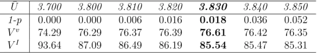
Table 2 describes the full opacity equilibrium. If voters were to demand 3.70 as the cutoff rule for reelection, the incumbent will always choose to follow the rule, that is, the probability of expropriation is zero. The PDV for incumbent and voter are 93.64 and 74.29 respectively.
Raising the bar to 3.80 per period makes no difference in the decision of the incumbent with respect to expropriation; even when there are some possible states of the world in which the incumbent should choose to expropriate, namely a combination of a bad shock
(θ=.8) and a very high level of outstanding debt, these states have a zero probability of occurrence.6 Accordingly, the PDV for incumbent and voter under a rule of 3.80 are 87.09
and 76.29, respectively.
Going beyond 3.80 progressively increases the probability of expropriation, but this does not necessarily mean that Vv will be lower since at first the marginal gains for
demanding a higher ¯U will dominate the losses in case of expropriation, given that 1−pis very low. As ¯U is increased, the second effect gains in importance over the first, reaching equilibrium at the point where they equal each other. The maximum is attained at ¯U∗ =
3.830 with a probability of expropriation of .018 and expected PDV for incumbent and voter equal to 85.54 and 76.61, respectively.
Table 2: Full Opacity Equilibrium Rule. ¯
U 3.700 3.800 3.810 3.820 3.830 3.840 3.850
1-p 0.000 0.000 0.006 0.016 0.018 0.036 0.052
Vv 74.29 76.29 76.37 76.39 76.61 76.42 76.35
VI 93.64 87.09 86.49 86.19 85.54 85.47 85.31
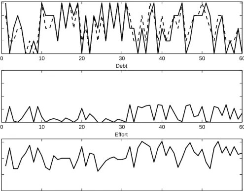
Figure 5 depicts policy paths under full opacity. Debt is more volatile and average debt is higher than in the dictatorship. Moreover, the incumbent incurs in higher levels of debt when θ is low and less productive, to help him fulfill the reelection rule. The correlation between d and θ is −0.83. In contrast to the other two cases, effort shows variability and can even be higher, in some periods, than in the full transparent case, although average effort is, of course, lower. Similarly to debt, the incumbent chooses higher levels of effort for lower levels of θ, being their correlations −0.87. In the figure we can see an expropriation period (and therefore a change of ruler) when effort reaches zero. In this case, expropriation occurs after a second consecutive worst shock.
3.4.3 The Intermediate cases: High Transparency, Low Transparency, and High Opacity
Consider the intermediate cases. Here, I am introducing a thirdde facto state variable: ˜θ. Voters now condition the reelection rule on the observed signal. I explore three distinct cases. High Transparency, a situation in which the signal is always informative; Low Transparency, a case where sometimes the signal is informative and; High Opacity, a circumstance in which the signal is almost never informative, and so it resembles Full
6Unless, of course, those are the initial conditions, but even in such case this can only happen for the
first government since the outstanding debt for the next government following expropriation will never be high enough.
Figure 5: Shock and Policy under Full Opacity. 0 10 20 30 40 50 60 0.8 0.9 1.0 1.1 1.2 Theta 0 10 20 30 40 50 60 0 0.1 0.2 0.3 0.4 Debt 0 10 20 30 40 50 60 0 0.5 1.0 1.5 2.0 Effort
Opacity. Figure 11 (see Appendix 2) shows how θ and ˜θ relate to each other depending
on ².
In the top panel of figures 6 and 7 it can be seen how θ and ˜θ move together across
time. Although ˜θ is a good approximation of θ with ² = .1 and a bad one when ² = .3.
By moving towards more opaque scenarios, these figures illustrate how debt and effort are progressively employed only to salvage office, rather than for efficiency reasons, which are
measured by the contemporaneous correlations of e and d with θ (look at the bottom of
top panel in table 3).
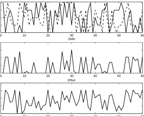
Figure 7 shows two periods of expropriation. The first episode coincides with the one obtained under full opacity. This episode would have being avoided if at least one of the signals had coincided with the true shock. The second episode is the consequence of two consecutive very uninformative signals, that make voters demand too much from the incumbent.
Figure 6: Shock and Policy under High Transparency. 0 10 20 30 40 50 60 0.8 0.9 1.0 1.1 1.2
Theta (solid), Signal (dashed)
0 10 20 30 40 50 60 0 0.1 0.2 0.3 0.4 Debt 0 10 20 30 40 50 60 0.6 0.8 1.0 1.2 Effort
3.5
Numeric Constraints
Transparency in the budgetary process is by no means the only force that conditions the realization of fiscal outcomes. In fact, the institutional arrangement that seems to capture most of the attention in the literature is the set of numeric rules that the executive has to face at the moment of elaboration, approval and execution of the budget. These numeric constraints can take the form of specific limits to expenditures, debt and deficit, or restrictions to the flow of resources between and within programs, agencies and levels of government. The constraints could even be restrictions to the flow of resources between different fiscal periods. The most extended use of a numeric constraint is an explicit cap on the budget deficit.
To incorporate this set of restrictions into the model, I condense them into a single de
jure budgetary rule. This allows me to evaluate, in the simplest manner, the effect these
rules can have when there are asymmetries in the information that players are receiving, and thus address the possibility that the government can escape legal consequences by exploiting financial loopholes. Specifically, I introduce a no-additional-debt rule that has to be observed by the incumbent with the same consequences as the minimum utility rule already imposed. That is, if the incumbent fails to fulfill it, he will be voted out of office in
Figure 7: Shock and Policy under High Opacity. 0 10 20 30 40 50 60 0.8 0.9 1.0 1.1 1.2
Theta (solid), Signal (dashed)
0 10 20 30 40 50 60 0 0.1 0.2 0.3 0.4 Debt 0 10 20 30 40 50 60 0 0.5 1.0 1.5 2.0 Effort
the following election. The problem with this rule, in contrast to the minimum utility rule, is that voters cannot directly observe the actual level of debt, but rather, they can only observe the reported level by the incumbent. Henceforth, I will call any deviation of the reported level from the actual levelcreative accounting. The extent to which the incumbent can use creative accounting as an instrument will be determined by the transparency level of the economy.
Formally, the no-additional-debt rule means that the incumbent would be reelected if, in addition to delivering ¯U, he also fulfils:
dt≤D(dt−1) (14)
At this point it is necessary to introduce more structure about howcreative accounting
can take place in the model. Following Milesi-Ferretti (2004) I assume that the extent of creative accounting is inversely related to the degree of transparency, but I do not attempt to derive it from within the model. This ad-hoc formulation is made for convenience. Otherwise, one would have to introduce more structure about effort which would be as arbitrary as directly modelling creative accounting. In particular, the game is modified by assuming that after the delivery of the public good, the government reports the amount
of debt that accrued during its production, ˜dt.
Figure 8: Timing of the Game.
t t+1 gt dt-1 Election t
θ
<
tθ
td
<
Any deviation from the true value of debt, that is if ˜dt6=dt,will be considered creative
accounting. To simplify, I assume that the government’s maximum amount of creative accounting without being caught is: dt±²dt, but that any attempt to engage in creative
accounting outside this interval will be detected by voters with probability one. For exam-ple, ²=.1 means that the government can falsely report up to 10 per cent of the period’s debt without being caught.
In terms of the model I then introduce theenforceable no-additional-debt rule: ˜
dt−err= (1−²)dt−err≤D(dt−1) (15)
For all positivedt−1 the maximum amount of possible diversion increases with ². The
term err, used for errors and omissions, is assumed to be constant across transparency and is needed in order to avoid a zero-debt trap: without err, once dt−1 reaches zero
the maximum amount of diversion is zero independently of the degree of transparency, something that would trivialize the solution. In any case, err is set to the minimum.7
Figure 8 shows how the rule affects policy decision. After observing gt and ˜dt, voters
learn if ¯U was satisfied and they have a rough idea of how much debt was utilized. After the (audited) value ofdt−1 is released voters also learn if the enforceable rule was satisfied.
In this game, a government is voted out for three possible reasons: If ¯U is not satisfied, if creative accounting is detected ( ˜dt <(1−²)dt), or if the enforceable no-additional-debt
rule is violated.
Even when the ad-hoc rule obviously makes it easier for opaque regimes to engage in creative accounting, it does not trivialize the outcome since the rule will be binding for some states in all regimes. That is to say, it imposes an effective cap on the per period
7The minimum errdepends on how fine the discrete state space is; the finer the grid the smaller err
will be, defined such that, if thedstate space consists of n points and we indexd bynwhere d(1) = 0,
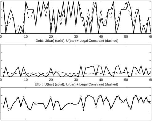
debt. This can be seen in figures 9 and 10. The imposition of this numeric rule modifies the government’s choice of optimal debt: even when debt moves in the same direction as in the unconstrained case—this is more pronounced as opacity increases—debt volatility is significantly reduced. In the constrained case debt is almost never as high as in the unconstrained case, but it is never as low either, reaching levels of zero debt only in the expropriation periods. Therefore, even when one should never expect to see debt levels as high as in the unconstrained case, this does not imply that average debt will be lower. The government finds it optimal to carry positive amounts of debt from period to period, since this gives it bigger room for engaging in creative accounting in order to smooth effort. In particular, in scenarios where there is no full transparency, the incumbent uses debt to fulfill the requirements and be reappointed, precisely in bad states of the world, when he is demanded relatively high levels of public good. But now the amount of debt that can be issued will be constrained by the amount outstanding last period, giving him the incentive to always carry over positive amounts of debt. This incentive will be enhanced as opacity increases.
Figure 9: Policy Comparison under High Transparency.
0 10 20 30 40 50 60 0.8 0.9 1.0 1.1 1.2
Theta (solid), Signal (dashed)
0 10 20 30 40 50 60 0 0.1 0.2 0.3 0.4
Debt: U(bar) (solid), U(bar) + Legal Constraint (dashed)
0 10 20 30 40 50 60
0.0 0.5 1.0 1.5
Figure 10: Policy Comparison under High Opacity. 0 10 20 30 40 50 60 0.8 0.9 1.0 1.1 1.2
Theta (solid), Signal (dashed)
0 10 20 30 40 50 60
0 0.1 0.2 0.3
0.4 Debt: U(bar) (solid), U(bar) + Legal Constraint (dashed)
0 10 20 30 40 50 60
0 0.5 1.0 1.5
2.0 Effort: U(bar) (solid), U(bar) + Legal Constraint (dashed)
3.6
The Effects of Transparency and Numeric Rules: Welfare,
Public Good, and Debt
The top panel of table 3 compares welfare, the average level of debt, and the average levels of public good, for the different degrees of transparency when no numeric rule is imposed. The bottom panel 3 does the same but including the no-additional-debt rule.
This exercises show, as in Ferejohn (1986), that more transparency is associated with an increase in welfare, driven by the average level of public good. The value added of the present setup is that is has been linked to public debt. Whereas in the long-run more transparency is always associated with lower levels of debt, in the short-run this is not always the case. For instance, by comparing Figures 6 and 7, it can be seen that between periods 10 and 20 the high transparency regime shows many periods with higher equilibrium debt than in the high opacity regime, for the same stream of shocks.
Contrasting the top and bottom panels of table 3, it can be seen that the the addition of the no-additional-debt rule does not necessarily imply a lower average debt across all regimes. In particular, whereas the highly transparent regime does reduce its average debt, the more opaque regimes increase average debt by non-insignificant magnitudes. Moreover, aside from the social planner case where it is obvious that debt and welfare has to decline,
the introduction of the numerical rule improves voter’s welfare in the highly transparent scenario and worsens it in the more opaque ones.
Table 3: Welfare, Public Goods, and Debt.
Descriptive Statistics: Only Transparency
Regime Dictator Social Full High Low High Full
Planner Transparency Transparency Transparency Opacity Opacity
Vv 59.93 83.20 82.47 80.71 78.11 77.01 76.61 gmean 2.92 4.18 4.12 4.05 3.97 3.89 3.89 dmean 0.047 0.047 0.00 0.050 0.065 0.072 0.087 emean 0.00 1.155 1.125 1.058 0.973 0.925 0.906 corr(e,θ) — — — -0.39 -0.63 -0.75 -0.87 corr(d,θ) 0.96 0.96 — -0.48 -0.64 -0.74 -0.83
Descriptive Statistics: Transparency and No-Additional-Debt Rule
Regime Dictator Social Full High Low High Full
Planner Transparency Transparency Transparency Opacity Opacity
Vv — 83.11 82.47 80.82 77.39 76.08 75.54 gmean — 4.17 4.12 4.06 4.00 3.91 3.91 dmean — 0.000 0.000 0.044 0.072 0.083 0.102 emean — 1.155 1.125 1.061 0.956 0.921 0.931 corr(e,θ) — — — -0.43 -0.71 -0.80 -0.93 corr(d,θ) — — — 0.07 -0.44 -0.54 -0.66
4
Empirical Evidence
The model presented in the first part of the paper has clear predictions about the amount of public goods produced and the level of debt incurred, for different degrees of budgetary transparency and the inclusion of numeric rules. While it would be very difficult to measure the delivery of public goods across countries, the data on public debt is readily available. For this simple reason, in this section I test the predictions of the model only on measures of debt. Additionally, measures of fiscal balance are also employed as dependent variable, since the level of public debt is reflecting the accumulation of deficits across time.
In concrete, the models’ predictions I want to test are:
• Countries with higher degree of budgetary transparency should exhibit lower levels of public debt and fiscal deficits.
• Numeric rules should induce lower levels of public debt and fiscal deficits only if budgetary transparency is sufficiently high.
To assess the effect of numerical rules and budgetary transparency on fiscal outcomes, I construct several indices of these budgetary institutions and then regress a series of fiscal outcome variables on these indices and other controls.
4.1
Measuring Transparency and Numerical Rules
The data for the construction of the indices was obtained from the OECD/World Bank
Survey of Budget Practices and Procedures (2003). The database contains more that 350 questions covering all sorts of issues about the budgeting process for 38 countries.8 I started
by selecting those questions that were directly related to transparency and numerical rules. From that set, I eliminated questions that were too similar—after corroborating that answers were the same—and I eliminated questions with ambiguous interpretations. At the end I ended up with 11 questions that were relevant to numerical rules and 14 questions for transparency.
To construct each index, every answer was given a value that ranged between zero and one, where higher values reflected institutions that should enhance fiscal discipline. Since, in general, questions had more than two answers, partial weights were proportionately distributed, following the method of Alesina et. al. (1999). Finally, the two indices were standardized so that each ranges from zero to one, which eased comparisons between them.
4.1.1 Transparency
How can one budgetary process be defined to be more transparent than other? Trans-parency is not a unidimensional concept; the literature contains many definitions that agree on the central issues of transparency, but authors assign different weights to its components, and omit others.
Based on the many definitions of transparency in the literature, Alt and Lassen (2003) try to rationalize and provide guidance of what a good measure of budgetary transparency would be. For this purpose they identify four main characteristics of transparency. First, more transparent procedures should process more information, and other things being equal, use fewer documents. This speaks to openness and ease of access and monitoring. Second, transparency is increased by the possibility of independent verification, which has been experimentally shown to be a key feature in making communication persuasive and credible. Third, there should be a commitment to non-arbitrary language: words and classifications should have clear, shared, unequivocal meanings. Finally, the presence of ex-ante more justification increases transparency, reducing the possibility of ex-post strategic justification.
To construct the transparency index, the following questions were employed, shown under the Alt and Lassen (2003) classification:
• More information, other things equal, in fewer documents
– Does the annual central government budget documentation submitted to the legislature/parliament contain multi-year expenditure estimates?
– At what interval is information on the in-year budget implementation released?
– Are the following accounts (assets, liabilities, government equity, revenues, ex-penses) integrated into the accounting system to facilitate the preparation of financial statements?
• Independent verification
– Does the government announce the release dates for information on the in-year budget implementation in advance?
– Are economic assumptions available for scrutiny?
– Is this information audited?
– Are audited final accounts published and available publicly?
– Are internal audit procedures clear and subject to effective process review by external auditors?
– Are the findings of the National Audit Body available to the public?
– Are government entities subject to financial audits by an external auditor? • Non-arbitrary language
– Does the government uses accrual accounting in its financial statements?
– Is there a unified accounting and budgeting classification system? • More justification
– Does the budget documentation contain a discussion of what impact variations in the key economic assumptions (sensitivity analysis) would have on the budget outturn?
– Does the published information have a comparison between actual and planned spending for the period covered?
The main transparency index has more weight on the verification side and in the type of information presented, and less on the amount of information per se. It seems more important to have fewer pieces of transcendental, bottom-lined and audited information at the relevant time than large amounts of data that might confuse rather than clarify the government objectives.
4.1.2 Numerical Rules
The possibility of running larger deficits or increasing the level of expenditures is, in principle, established in the legislation. Other things being equal, one should observe higher fiscal deficits or debt levels the less constrained is the budgetary process. Note, however, that the model presented in the first part of the paper establishes that the effects of numerical rules on fiscal outcomes depend on the level of transparency.
Ideally it would be possible to distinguish between restrictions to the overall budget and to the composition of it and, presumably, only the first type should affect aggregate fiscal outcomes. In practice, such separation might not exist; budgetary processes that allow inter program transfers, for instance, can create a bigger budget by ex-ante inflating accounts or programs that are not so carefully watched in comparison to others and then making ex-post transfers. If this type of connection is of true importance or just a second order effect is a question that I try to answer here. For this reason, the questions used to construct the numerical constraint index were separated in three categories: those that refer to direct restrictions to the overall budget, those that refer to transfers within the fiscal budget, and those that refer to transfers between different budgetary years.
• Direct Restrictions
– In developing the budget, are there fiscal rules placing limits on Executive fiscal policy discretion?
– Can you change expenditures outside the budget process? • Between Restrictions
– Is it possible to carry-over unused appropriations for operating costs (salaries, etc.) from one year to another?
– Is it possible to carry-over unused appropriations for investments (building con-struction, etc.) from one year to another?
– Is it possible to carry-over unused appropriations for transfer programs from one year to another?
– Is it possible for managers of ministries/government organizations to borrow against future appropriations for operating costs (salaries, etc.)?
– Is it possible to borrow against future appropriations for investments (building construction, etc.)?
• Within Restrictions
– Are there laws, regulations or policies that define the permitted uses of the budget reserves and the decision-making authorities for approving allocations from the reserves?
– Are government organizations allowed to transfer funds between operating ex-penditures, investments and program funds?
– Can appropriations be reallocated from one program to another?
– More generally, are transfers permitted between capital investments or transfer programs (social security pensions, etc.) and operating expenditures?
I compute three main numerical constraints indices. The first one assigns equal weight to each question which implicitly gives more importance towithin andbetween constraints since both represent nine out of eleven questions. Two additional measures are then com-puted to tackle this problem. The second index gives half the weight todirect restrictions and the other half to the within and between constraints. The third index disregards the within and between effects concentrating only on direct constraints.
4.2
The Effects of Budgetary Institutions on Fiscal Outcomes.
This section presents a series of econometric models that try to answer the question of how different budgetary institutions, in the form of the constructed indices, affect fiscal outcomes across countries. First, I introduce the benchmark model, which controls for economic and demographic variables that has been shown to affect fiscal outcomes. Sec-ond, I study possible differences in the estimated parameters, depending on the degree of development of the countries in the sample. Finally, I add to the model a series of political variables that can also affect fiscal outcomes.
4.2.1 Data and the Benchmark Model
Fiscal outcomes variables come from the World Economic Outlook (WEO), produced by the International Monetary Fund, and were constructed as averages of the period 1999-2003. All the remaining economic and population variables are directly extracted, or constructed from, the World Development Indicators (WDI). The political variables are from theDatabase of Political Institutions (DPI2004) by Philip Keefer (District Magnitude
andNumber of Effective Parliamentary Parties), and from The Economist (Cabinet Size). The empirical strategy is to fit the following benchmark model:
F O =β0+β1T ransparency+β2NumericalRules+β3Hierarchical+β~0X+², (16)
whereF O, that stands forFiscal Outcomes, can alternatively take the form ofGeneral Bal-ance, Central BalBal-ance, General Net Debt, and General Gross Debt, all expressed as ratios
to GDP and, as was mentioned earlier, averaged over the 1999-2003 period. T ransparency
and NumericalRules are the computed institutional indexes that were described in the previous subsection. Hierarchicalis an index trying to measure the third budgetary insti-tution recognized in the literature, procedural rules, and was constructed in a similar way as the other two indexes.9 X is a vector of economic and demographic control variables
that can potentially influence fiscal outcomes. The controls are, first, the average growth of GDP for the 1990-2003 period (Avg. Growth) which is believed to be directly related to revenues due to the progressivity of the tax structure and higher tax revenues from job creation, and inversely (or neutrally) related to expenditures, due to lower unemployment benefits paid by the state. Added together, these should have a positive effect on fiscal balances and a negative effect on public debt. Second, the Dependency Ratio, defined as the sum of population under 12 and over 65, divided by total population and averaged over the 1999-2003 period, is expected to have the opposite effects to Avg. Growth on fiscal outcomes since a higher dependency ratio represents a lower taxable base on one hand, and higher expenditure on education and in the pension system, other things being equal. The third variable (Wagner) is the average GDP per capita over the 1999-2003 period, measured in dollars and adjusted by PPP, that is used as a proxy for the country’s development level. This variable controls for Wagner’s law, the prediction of a positive correlation between the development level of an economy and it’s share of public expendi-ture to GDP. It is important to note that this variable may be correlated with budgetary institutions. However, all the results that are reported below are robust to the exclusion of the Wagner variable from the benchmark model. Additionally, I have conducted another exercise splitting the sample according to the development level of countries, in order to account for this potential source of bias. The last control is the degree of openness of an economy, defined as the ratio of the sum of total exports and total imports to GDP (Openness). This variable is included to account for the empirical finding (Rodrik (1996)) that more open economies tend to have larger levels of government. I have also included the value of the dependent variable in 1990 as a control for the evolution of the analyzed fiscal outcome during the last decade.
There are two potential problems with the econometric specification. The first one is endogeneity: In the literature, and this work is no exception, budgetary institutions are
9Procedural rules dictate the timing and mechanisms by which the executive drafts the budget, it’s
discussion and approval in the legislature, and its posterior implementation. These procedural rules determine the relative strength of the players involved in the budgeting process within the executive and between the executive and the legislature. In this literature, procedural rules are classified on a hierarchical-collegial spectrum. At the stage of budgeting drafting, hierarchical rules are those that tilt the balance of power in favor of the finance minister, who faces the whole government budget constraint, and in detriment of spending ministers, who care almost exclusively about their own portfolio. On the contrary, collegial rules are those in which the role of the finance minister is more passive and limited. At the approval stage, hierarchical rules are those that impose more constraints on the legislature’s ability to modify the budget proposed by the executive, and in particular, on its ability to increase the size of the budget or the deficit. At the execution stage, hierarchical rules are those that limit the possibility of the legislature to increase the budget once it has been approved.
treated as being exogenous, while it is also recognized that they are indeed endogenous, particularly to past fiscal outcomes. The justification to this treatment is that, at least in the short run, institutions are reasonably difficult to change, and therefore are changed relatively infrequently. Since it is costly and complex to change institutions, the existing ones have to be very unsatisfactory before it is worth changing them; as a result, there is a strong “status quo” bias in institutional reform. Therefore, at least up to a point, one can use institutional features as explanatory variables (Alesina and Perotti (1999)). The second problem is the potential correlation between the budgetary institutional variables. Indeed, while the simple correlation between transparency and the other two measures of budgetary institutions is not different from zero, the Hierarchical and Numerical Rules
variables are positively correlated. I used different definitions for Numerical Rules and also drop the Hierarchical variable to account for this problem, and the results remain qualitatively the same.
The benchmark results for Central Balance, General Balance, General Net Debt, and
General Gross Debt are presented in table 4. For each fiscal outcome, the model with only the economic controls, is reported on the left columns, and the economic controls and budgetary institutions on the columns of the right.
Looking at the models with the economic controls alone, there are two aspects that are worth mentioning. First, in none of the four fiscal outcomes analyzed are all of the economic controls significant at the same time but, nevertheless, we can confidently reject the null of all coefficients being jointly equal to zero. Moreover, every economic control enters significantly in at least half of the fiscal outcomes analyzed. Second, all the economic controls that enter significantly in each equation, does it with the expected sign, although some of them lose significance once the budgetary variables are included in.10
Looking at the columns on the right in table 4 for each fiscal outcome, it can be seen that budgetary transparency helps to explain the cross-country differences of all fiscal outcomes, although the effect seems to be stronger for the debt variables than for the fiscal balance variables. At the same time, it can also be seen that numerical rules do not enter significantly in any of the regressions. These results are congruent with the model presented in the previous section.
The interpretation of the point estimates of Transparency is that an increase in this variable of one standard deviation (0.12) from its midpoint (0.69) is associated with, rel-ative to GDP, a fiscal stance improvement of 1.2 and 1.6 percent on Central and General Balance, and with a 10.4 and 12.4 percent reductions in General Net Debt and General Gross Debt, respectively. In terms of the explained cross country variation, the inclu-sion Transparency in the benchmark model improves considerably the R-squared of the
10Dropping one control at a time did not change the significance level of any of the other variables.
Their coefficient values never changed more than 5%. Since there are good theoretical motives to suspect that the non-significant controls truly affect fiscal outcomes they are left as part of the regression.