http://dx.doi.org/10.4236/ojs.2015.51011
Comparison of Uniform and Kernel Gaussian
Weight Matrix in Generalized Spatial Panel
Data Model
Tuti Purwaningsih, Erfiani, Anik Djuraidah
Departement of Statistics, Graduate School of Bogor Agricultural University, Bogor, Indonesia Email: [email protected]
Received 7 February 2015; accepted 25 February 2015; published 28 February 2015
Copyright © 2015 by authors and Scientific Research Publishing Inc.
This work is licensed under the Creative Commons Attribution International License (CC BY). http://creativecommons.org/licenses/by/4.0/
Abstract
Panel data combine cross-section data and time series data. If the cross-section is locations, there is a need to check the correlation among locations. ρand λ are parameters in generalized spatial model to cover effect of correlation between locations. Value of ρor λwill influence the goodness of fit model, so it is important to make parameter estimation. The effect of another location is covered by making contiguity matrix until it gets spatial weighted matrix (W). There are some types of W—uniform W, binary W, kernel Gaussian W and some W from real case of economics condition or transportation condition from locations. This study is aimed to compare uniform W
and kernel Gaussian W in spatial panel data model using RMSE value. The result of analysis showed that uniform weight had RMSE value less than kernel Gaussian model. Uniform W had stabil value for all the combinations.
Keywords
Component, Uniform Weight, Kernel Gaussian Weight, Generalized Spatial Panel Data Model
1. Introduction
condi-tion, for that need, a model that involves spatial influence in the analysis panel data will be mentioned as Spatial Panel Data Model.
Some recent literature of spatial cross-section data is Spatial Ordinal Logistic Regression by Aidi and Purwa-ningsih [2], and Geographically Weighted Regression [3]. Some of the recent literature of Spatial Panel Data is forecasting with spatial panel data [3] and spatial panel models [4]. For accomodating spatial dependence in the model, there is spatial weighted matrix
( )
W that is an important component to calculate the spatial correlation between locations. Spatial parameter in generalized spatial panel data model, is known as ρ or λ. There are some types of W —uniform W, binary W , inverse distance W and some W from real cases of econom-ics condition or transportation condition from the area. This research is aimed to compare uniform W and kernel Gaussian W in generalized spatial panel data model using RMSE value which is obtained from simulation.2. Literature Review
2.1. Data Panel Analysis
Data used in the panel data modelisa combination of cross section and time-series data. Crossection data is data collected at one time of many units of observation, then time-series data is data collected over time to an obser-vation. If each unit has a number of observations a cross individuals in the same period of time series, it is cal-leda balanced panel data. Conversely, if each individual unit has a number of observations a cross different pe-riod of time series, it is called an unbalanced panel data (unbalanced panel data).
In general, panel data regression model is expressed as follows:
1, 2, , ; 1, 2, ,
it it it i N t
y =α+x′β+u = = T (1)
with i is an index for crossection data and t is index of time series. α is a constant value, β is a vector of size K×1, with K specifies the number of explanatory variables. Then yit is the response to the individual cross-i for all time period stand xit are sized K×1 vector for observation i-th individual cross and all time periods t and uit is the residual/error [5].
Residual components of the direction of the regression model in Equation (1) can be defined as follows:
it i it
u =µ ε+ (2)
where µi is an individual-specific effect that is not observed, and εit is a remnant of crossection-i and time series-t[5].
2.2. Spatial Weighted Matrix (W)
Spatial weighted matrix is basically a matrix that describes the relationship between regions and obtained by distance or neighbourhood information. Diagonal of the matrix is generally filled with zero value. Since the weighting matrix shows the relationship between the overall observation, the dimension of this matrix is N × N
[6]. There are several approaches that can be done to show the spatial relationship between the location, includ-ing the concept of intersection (contiguity). There are three types of intersection, namely Rook Contiguity, Bi-shinop Contiguity and Queen Contiguity [6].
After determining the spatial weighting matrix to be used, further normalization in the spatial weighting trix. In general, the matrix used for normalization normalization row (row-normalize). This means that the ma-trix is transformed so that the sum of each row of the mama-trix becomes equal to one. There are other alternatives in the normalization of this matrix is to normalize the columns of the matrix so that the sum of each column in the weighting matrix be equal to one. Also, it can also perform normalization by dividing the elements of the weighting matrix with the largest characteristic root of the matrix ([6] [7]).
( ) 1
, is neighbor of in -th order
0, others
l ij ni
j i l
W = (3)
( )l i
n is the number of neighbor locations with site-i in -th order. The non-uniform weight may become uni-form weight when some conditions are met. One method in building non-uniuni-form weight is based on inverse distance. The weight matrix of spatial lag k is based on the inverse weights 1 1
(
+dij)
for sites i and j whose Euclidean distance dij lies within a fixed distance range, and otherwise is weight zero. Kernel GaussianWeight follow this formulla:
( )
(
)
2exp 1 2
j ij
w i = − d b (4)
with d isdistance between location i and j, then b is bandwith which is a parameter for smoothing function.
2.3. Generalized Spatial Panel Data Model
Generalized spatial model expressed in the following equation:
1 dengan 1
N N
it j ij jt it i it it j ij it it
y =ρ
∑
= w y +x′β+µ φ+ φ =λ∑
= wφ +ε (5)where ρ is spatial autoregressive coefficient, wij is elements of the spatial weighted matrix which has been normalized
( )
W and λ is spatial autocorrelation between error [7].3. Methodology
Data used in this study was gotten from simulation using generalized spatial panel data model as Equation (5) with initiation of some parameter. Simulation was done use R program. The following step is used to generate the spatial data panel which is consist of index n and t. In dexnindicates the number of locations and indextindi-cates the number of period in each locations. Here is the proccess:
1) Determining the number of locations to be simulated is N=3, N=9 and N =25. 2) Makes 3 types of map location on step 1.
3) Creating a binary spatial weighted matrix based on the concept of queen contiguity of each type of map lo-cations. In this step, to map the 3 locations it will form a 3 × 3 matrix, 9 locations will form a 9 × 9 matrix and 25 locations form a 25 × 25 matrix.
4) Creating spatial uniform weighted matrix based on the concept of queen contiguity of each type of map lo-cations.
5) Making weighted matrix kernel Gaussian based on the concept of distance. To make this matrix, previously researchers randomize the centroid points of each location. After setting centroid points, then measure the dis-tance between centroids and used it as a reference to build kernel Gaussian W. Gaussian kernel W as follows:
( )
1(
)
2exp 2
j ij
w i = − d b
[3].
6) Specifies the number of time periods to be simulated is T =3, T =6, T =12 and T =24.
7) Generating the data Y and X based on generalized spatial panel data models follows Equation (5). 8) Cronecker multiplication between matrix identtity of time periods and W, then get new matrix named IW. 9) Multiply matrix IW and Y to obtain vector WY.
10) Build a spatial panel data models and get the value of RMSE.
11) Repeat steps 7)-9) until 1000 replications for each combination on types of W, N, T , ρ and λ. Description:
Types of W: W binary, W uniform and Gaussian kernel W; Types of N: 3, 9 and 25 locations;
Types of T: 3, 6, 12 and 36 series;
Types of ρ=0.3, 0.5, 0.8 and λ=0.3, 0.5, 0.8.
13) Determine the best W based on the smallest RMSE for all combinations.
4. Results and Discussions
[image:4.595.93.536.194.722.2]Simulation generate data for vector Y as dependent variable and X matrix as independent variable. Y and X is generate with parameter initiation. After doing simulation, we can get RMSE for each combinations and proccessing it, then we can calculate RMSE for each W, N, T, ρ and λ. Here is the result. With the result in
Table 1 then continued to figure it into graphs in order to look the comparison easily.
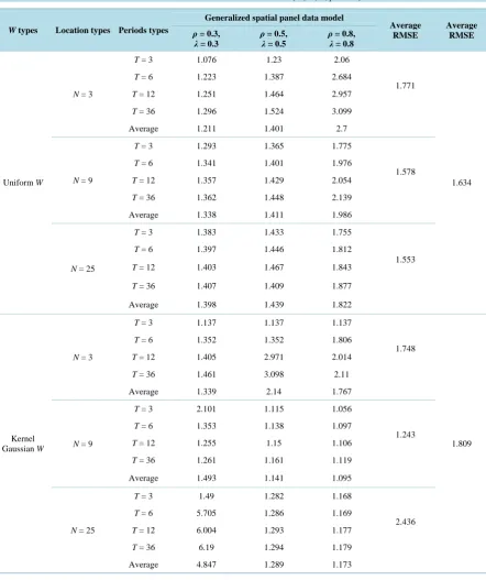
Table 1.Value of RMSE resulted from simulation for all the combinations (W, N, T, ρ and λ).
W types Location types Periods types
Generalized spatial panel data model
Average RMSE
Average RMSE ρ = 0.3,
λ = 0.3 ρ = 0.5, λ = 0.5 ρ = 0.8, λ = 0.8
Uniform W
N = 3
T = 3 1.076 1.23 2.06
1.771
1.634 T = 6 1.223 1.387 2.684
T = 12 1.251 1.464 2.957
T = 36 1.296 1.524 3.099
Average 1.211 1.401 2.7
N = 9
T = 3 1.293 1.365 1.775
1.578 T = 6 1.341 1.401 1.976
T = 12 1.357 1.429 2.054
T = 36 1.362 1.448 2.139
Average 1.338 1.411 1.986
N = 25
T = 3 1.383 1.433 1.755
1.553 T = 6 1.397 1.446 1.812
T = 12 1.403 1.467 1.843
T = 36 1.407 1.409 1.877
Average 1.398 1.439 1.822
Kernel Gaussian W
N = 3
T = 3 1.137 1.137 1.137
1.748
1.809 T = 6 1.352 1.352 1.806
T = 12 1.405 2.971 2.014
T = 36 1.461 3.098 2.11
Average 1.339 2.14 1.767
N = 9
T = 3 2.101 1.115 1.056
1.243 T = 6 1.353 1.138 1.097
T = 12 1.255 1.15 1.106
T = 36 1.261 1.161 1.119
Average 1.493 1.141 1.095
N = 25
T = 3 1.49 1.282 1.168
2.436 T = 6 5.705 1.286 1.169
T = 12 6.004 1.293 1.177
T = 36 6.19 1.294 1.179
Figure 1.Comparison of RMSE between uniform W and kernel Gaussian W
[image:5.595.148.479.81.430.2] [image:5.595.172.456.87.256.2]for all combinations.
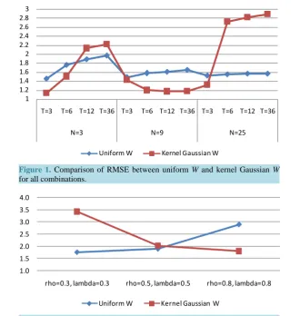
Figure 2. Comparison RMSE each W for each parameter.
Based onFigure 1 can be said that uniform W has smaller RMSE than kernel Gaussian W for T = 12, T = 36 on location N = 3, then for T = 6, 12, 36 on location N = 25 and the remaining combinations, kernel Gaussian is higher. If we look the level of stabilization, uniform W is better than kernel Gaussian W. We can look ats the graph in blue line as uniform W, it has value only in range 1, 4 until 2 then kernel Gaussian W has range from 1 - 3. So can be concluded that uniform W is better than kernel Gaussian W.
Based on Figure 2, we can look that average RMSE of uniform W is smaller in ρ=0.3, λ =0.3 and 0.5
ρ= , λ=0.5 while kernel Gaussian W is smaller only in ρ=0.8, λ=0.8.
5. Conclusion
After looking at the result, it can be concluded that uniform W is better than kernel Gaussian W almost for all combinations of N and T. Then uniform W is better in ρ and λ in small value until medium (less than 0.5).
Acknowledgements
The first, authors would like to thankful to Allah SWT, my parents, lecturer and all of friends. This research was supported by private funds.
References
[1] Anselin, L., Gallo, J. and Jayet, H. (2008) The Econometrics of Panel Data. Springer, Berlin.
[2] Aidi, M.N. and Purwaningsih, T. (2012) Modelling Spatial Ordinal Logistic Regression and the Principal Component to Predict Poverty Status of Districts in Java Island. International Journal of Statistics and Application, 3, 1-8.
[3] Fotheringham, A.S., Brunsdon, C. and Chartlon, M. (2002) Geographically Weighted Regression, the Analysis of
Spa-1 1.2 1.4 1.6 1.82 2.2 2.4 2.6 2.83
T=3 T=6 T=12 T=36 T=3 T=6 T=12 T=36 T=3 T=6 T=12 T=36
N=3 N=9 N=25
Uniform W Kernel Gaussian W
1.0 1.5 2.0 2.5 3.0 3.5 4.0
rho=0.3, lambda=0.3 rho=0.5, lambda=0.5 rho=0.8, lambda=0.8
tially Varying Relationships. John Wiley and Sons, Ltd., Hoboken.
[4] Elhorst, J.P. (2011) Spatial Panel Models. Regional Science and Urban Econometric.
[5] Baltagi, B.H. (2005) Econometrics Analysis of Panel Data. 3rd Edition, John Wiley and Sons, Ltd., England.
[6] Dubin, R. (2009) Spatial Weights. In: Fotheringham, A.S. and Rogerson, P.A., Eds., Handbook of Spatial Analysis, Sage Publications, London. http://dx.doi.org/10.4135/9780857020130.n8