DYNAMIC SENSOR RELOCATION TECHNIQUE BASED LIGHT WEIGHT INTEGRATED PROTOCOL FOR WSN

ISSN: www.jatit.org E-ISSN:

SIMULATED ANNEALING ALGORITHM USING ITERATIVE

COMPONENT SCHEDULING APPROACH FOR CHIP

SHOOTER MACHINES

MANSOUR ALSSAGER a, ZULAIHA ALI OTHMAN b

a,b

Faculty of Information Science and Technology, University Kebangsaan Malaysia 43600 Bangi, Selangor Darul Ehsan, Malaysia

ABSTRACT

A Chip Shooter placement machine in printed circuit board assembly has three movable mechanisms: an X-Y table carrying a printed circuit board, a feeder carrier with several feeders holding components and a rotary turret with multiple assembly heads to pick up and place components. In order to minimize the total traveling time spent by the head for assembling all components and to reach the peak performance of the machine, all the components on the board should be placed in a perfect sequence, and the assembly head should retrieve or pick up a component from a feeder that is properly arranged. There are two modeling approaches of solving the components scheduling problem: integrated and iterative approaches, most popular meta-heuristic used so far for components scheduling problem is population based using integrated modeling approach. This work presents a single based meta-heuristic known as Simulated Annealing with an iterative modeling approach was adopted. The computational study is carried out to compare other population-based algorithms that adopted integrated approach. The results demonstrate that the performance of the simulated annealing algorithm using iterative approach is comparable with other population-based algorithms using integrated approach.

Keywords: Printed Circuit Board, Chip Shooter Machine, Simulated Annealing.

1.INTRODUCTION

This study focuses on the single machine scheduling problem in printed circuit boards (PCBs) assembly, an important process in the electronics industry. The PCB assembly process in surface mount technology (SMT) environment consists of five operations:

• Applying solder paste where the components should be placed (Screen Printing).

• Placement operation which performed by high-speed placement machine to mount small components such as chip resistors which preferably mounted first on the PCB, then flexible placement machine is used to mount the larger component's such as integrated circuit (ICs) on the PCB.

• Inspection operation is performed to ensure all the components have been placed in the right manner.

• Then the PCB is conveyed through an oven to make the solder paste reflow and form the solder joints.

• Finally the PCB is cleaned from contaminants exposed during the assembly process.

Components placement machines in SMT environment can be categorized into five types with

each placement machine possesses its own specifications as well as operations; these being dual-delivery, multi-station, turret-type, multi-head and sequential pick-and-place SMD placement machines (Ayob & Kendall 2008). This study focuses on turret-type assembly machine also known as concurrent chip shooter (CS), where the major advantage of this CS machine is its high speed because all the parts such as the feeder carrier with several feeders holds the components, X-Y table carrying the PCBs, rotary multiple head turret pick up and place the components (Leu et al. 1993; Ayob & Kendall 2008) are moving concurrently. However, CS machine is only preferable for operations with small components such as chip resistor (Ho & Ji 2007; Ayob & Kendall 2008; Ho & Ji 2009). Usually CS machine is arranged first in the assembly line because the placement of small components is given priority before the large one in assembly operation.

ISSN: www.jatit.org E-ISSN:

motivates the PCB manufacturer to optimize the assembly processes in order to either minimize the total production cost or maximize the profit (Crama et al. 1997; Moyer & Gupta 1997). Many meta-heuristics have been successfully applied to components scheduling problem in PCB, however they are focused on population based solution, and less research conducted to explore the potential of a single based solution to address the problem. The simulated annealing algorithm is proposed to solve the problem mainly using iterative approach.

Based on the recent literatures review shown, it is the fact that still less researchers looking at the potential of an iterative modelling approach for the PCB scheduling problem of CS machine. Genetic algorithm is the most used by the researchers (Leu et al. 1993; Ong & Tan 2002; Ho & Ji 2006; Ho & Ji 2009) and they enhanced the algorithm using various local searches algorithm to reduce complexity of the algorithm. SA is well-known as a simple algorithm that is able to solve various problems such as in TSP, time-tabling, etc. SA has proven to be able to solve various domain problems, too. Therefore, applying SA in PCB using appropriate local search is believed to be able to solve PCB.

This paper is organized as follows: Section 2 discusses the basic concept of PCB, the state of the art on PCB’s solution and the experiment conducted. Section 3 shows the result and performance of SA used to solve PCB using integrated and iterative approaches compared with other population based algorithms. Lastly the last section concluded the research result.

2.MATERIAL AND METHODS

2.1.Chip Shooter Machine

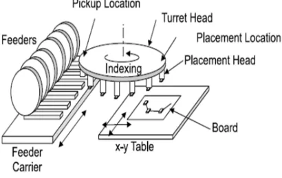
In a high-speed CS machine (see Figure 1), the component placement heads are at a fixed-axis turret. The PCB is held onto a moving x-y table that moves the PCB to locate the appropriate placement point under the placement head. The component feeders are located on a moving feeder carrier, which moves the feeders to the pickup location. The components are picked up from the feeder, rotated on the turret and finally placed on the board. The time delay refers to the time lag of each components pick up and placement due to the rotation on the turret head. The mechanism that takes the longest time to complete the operation

dictates the placement time. The arrangement of the feeders and the placement sequence of the components are the two important factors of the scheduling problem. Since the machine operates in a concurrent manner, many researchers highlight the need to incorporate this concurrency in the solution approach (Nelson & Wille 1995; Ong & Tan 2002; Ayob & Kendall 2005; Ho & Ji 2006; Ho & Ji 2007; Ayob & Kendall 2008; Ang et al. 2009; Ho & Ji 2009). However, solving the problem individually rather than simultaneously is still prevalent, nevertheless no recent studies investigate the iterative approach further. As mentioned the PCB scheduling problem on the CS machine can be further broken down into two sub-problems. First, a feeder assignment problem to determine a suitable arrangement to assign a set of components types to feeders with minimum assembly time. Next, a sequencing problem determines to a suitable sequence of pick-and-place movements of the turret. Since both problems are somewhat similar to the Travel Salesman Problem (TSP) with Chebyshev distance measure and Quadratic Assignment Problem (QAP), as many researchers modeled them (Leu et al. 1993; Duman 1998; Duman 2005; Ho & Ji 2007), the integrated problems are extremely complicated.

The objective of solving PCB scheduling problem is to minimize the placement time, which is the summation of all dominating times of components where the dominating time is the longest one among the three times in one step. In this study, Simulated Annealing (Soneji & Sanghvi) is proposed, that sequentially and independently solves the component sequencing and feeder arrangement problems where one of the problems is tackled in advance, followed by the other problem with respect to the first problem solution.

ISSN: www.jatit.org E-ISSN:

2.2.PCB Solution

A variety of research has been conducted on optimizing the performance of PCB placement machines. Some researchers address the feeder arrangement and the components sequencing problem independently using iterative approach. However, this approach cannot guarantee that the solution is globally optimal (Ho & Ji 2007), whilst others address the problem as an interrelated problem using integrated approach, where the two problems are tackled concurrently.

(Leu et al. 1993) presented a genetic algorithm approach for the component sequencing and feeder arrangement problem, which solved the problems using fundamental genetic algorithm with four genetic operators, simultaneously: crossover operator, inversion operator, rotation operator, and mutation operator. The performance of the algorithm is weak in CS machine compared to the latest study. (Nelson & Wille 1995) proposed an evolutionary programming algorithm with emphasis on phenotypic behaviour, however this method is similar to genetic algorithm in some aspects, where the mechanism was used is very simple, only one type of mutation used, and the study reported that this method is able to produce a good quality solution in comparable time using integrated approach and compared against genetic algorithm. (Moyer & Gupta 1997) developed a heuristic algorithm for determining the component sequencing and the feeder arrangement problems, individually. (Ong & Tan 2002) proposed genetic algorithm method using integrated modeling with several improving heuristic: order crossover, position based crossover, and order based crossover, inversion mutation, pairwise swap, insertion mutation, and displacement mutation. The algorithm engages a two-stage genetic operation, mating of the component chromosomes and mating of the feeder chromosomes. This approach has improved the overall fitness value of the parent space faster than basic genetic algorithm proposed by (Leu et al. 1993). Recently, (Ho & Ji 2009) develop a new integrated mathematical model and successfully applied the model using hybrid genetic algorithm with three heuristics: nearest neighbor, 2-opt local search and iterated swap procedure to solve the two problems of CS machine concurrently. The study shows that the larger population size can obtain better quality solution, and the result of the algorithm was better than

genetic algorithm, which was proposed by (Ong & Tan 2002).

3.PROPOSED SIMULATED ANNEALING

FOR PCB

Simulated Annealing (Soneji & Sanghvi) is a stochastic optimization technique developed by (Kirkpatrick et al. 1983), starts with one initial solution, then the solution evolves through successive iterations. During iteration, the solution is evaluated using some measures of fitness. The fitter the solution, the higher the probability of being selected to be further enhanced. Accepting the worse solution is maintained by the diversity in the population and avoided being trapped in a local optimum. After the predetermined number of iterations is performed, the algorithm converges to the best solution, which hopefully represents the optimal solution or may be a sub-optimal solution to the problem. SA shows a good adaptability for many combinatorial optimization problems, and is applied widely to engineering industry because of simplicity; easy operation and great flexibility have prompted this study to apply SA to solve the PCB problem.

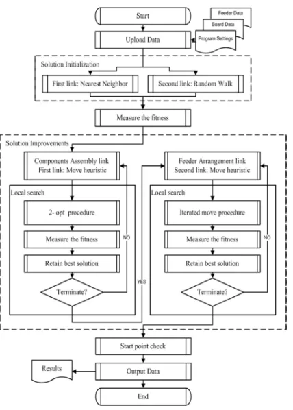
The flowchart of the proposed Simulated Annealing for the combined problems is illustrated in Figure 2. The algorithm incorporates four heuristics: nearest neighbor, move, 2-opt and iterated move heuristics. The procedure of SA is described as follows: After the SA parameters have been set; SA generates the initial solution to the problem. The solution contains two segments or links. The first link represents the sequence of the component placements, whereas the second link represents the arrangement of the component types to feeders. Firstly, the nearest neighbor heuristic (NNH) is applied for generating the first link, whereas, the second link is generated randomly.

ISSN: www.jatit.org E-ISSN:

first link unless the predetermined number of iterations is conducted. However the ending of the first link improvements is the start of the second link improvements, the best solution obtained from the first improvement stage is used in the second stage to improve the feeder assignment. The feeder improvement stage starts by the move heuristic, a new solution is produced, and then the iterated move procedure are used to improve the solution further as a local search to obtain a better quality solution. The solution is examined by an evaluation function, and only the best quality solution is retained, that’s form a one iteration of feeder improvements. A predetermined number of iteration is conducted until the stop condition is satisfied. By ending the stage, the improvements process is finished and the best solution is reported. The detailed algorithm is discussed in the following sections.

Figure 2: Simulated Annealing Flow Chart

3.1.Encoding

The solution is encoded based on one-dimensional array consisting of two segments component assembly link and feeder arrangement link as shown in Figure 3. The component link

represents the component placement sequence. This is an array of numbers, which represents the placement sequence in the placement order. The numbers represent the component numbers. These component numbers will provide the corresponding x- and y-coordinates and the component type, from the board data. The feeder arrangement sequence is represented in the feeder link, in sequential order. The numbers correspond to the feeder number. The feeder numbers provide the corresponding feeder widths and component types.

3.2.Evaluation

The fitness function of the component assembly problem should be the total assembly time, which is the summation of all dominating times of the components. It is due to the three mechanisms of the CS machine motion at different speeds, such as the traveling time of the PCB or the X–Y table, the traveling time of the feeder carrier, and the indexing time of the turret. The longest one among the three is the dominating time needed in the assembly of the component, as discussed earlier. Let Ti be the time needed for the placement of component i and Ttotal be the total assembly time or the fitness function for solution Xh in the component assembly problem, then

Where t1(a, b) is the traveling time of the X–Y table from component a to component b

For Chebyshev metric, vx is the speed of the X–Y table in the x direction, vy is the speed of the X–Y table in the y direction, t2 (u, v) is the traveling time of the feeder carrier from feeder u to feeder v

where vf is the speed of the feeder carrier, t2 is the indexing time of the turret, n is the number of components, ci is the location in the board for the ith

(

)

f

f i f j f i f j

v

x x x x v u t

2 2

2 ,

− + − = Component Assembly

Components number Feeder Arrangement Components type

c1 c2 …. …. cN-1 cN t1 _t3 _t4

t1 t2 …. …. t5 t1 _f1 _{…. f}R-1

Components type Slot number

Figure 3: Representation of a PCB Assembly Solution

(

)

(

)

(

)

maxt c c t f f t

Ti = i− i i+g− i+g

(

)

  

 

 _{− −}

= − −

y i i

x i i

v y y v

x x b

a

t 1 1

1 , max ,

∑

=

N

i i total T

T

ISSN: www.jatit.org E-ISSN:

component, fi is the feeder location for the ith component type, and g is the number of components in the gap between the pick-up component and the placement component in the turret.

3.3.Initialization Heuristic

Although the component assembly problem is simple to describe, it is very difficult to solve optimally when the number of components or the problem size is large. Therefore using heuristic technique in initialization is very helpful in such situation. In SA, one type of heuristics is adopted to initialize the solution, which is the Nearest Neighbor Heuristic (NNH) used to initialize the first link, whereas the second link is initialized randomly.

3.3.1.Nearest neighbor heuristic

NNH is used to generate an initial solution for the first link only, which is the sequence of the components placement. The principle of NNH is to start with the first component randomly, then to select the next component as close as possible to the previous one from those unselected components to form the placement sequence until all components are selected.

3.4.Construction Heuristic

The construction heuristics used in SA are move heuristic for both segments and two local search heuristics, 2-opt heuristic for components sequencing link and iterated move procedure for feeder arrangements link. The two links of the solution are required to perform these construction heuristics. The number of construction heuristics performed to the solution depends on the temperature and cooling rate, which are predetermined in advance.

3.4.1.The move heuristic

The move heuristic adopted in SA is shown in Figure 4. The procedure simply selects two random indexes, removes the request from the first random index and reinserts it at the second random index to form a new neighbor solution. This heuristic is used for the two problems.

1 2 3 4 5 6 7 8 9 Old solution 1 2 8 3 4 5 6 7 9 New solution

Figure 4: The Adopted Move Heuristic Procedure

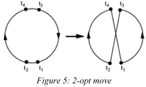
3.4.2.2-opt procedure

Next to follow is the 2-opt local search, where the principle of the 2-opt heuristic is very straightforward. Its work by systematically exchange the assembly sequence direction between two pairs of consecutive components is the assembly sequence, and evaluate whether the assembly time of the components assembly sequence is improved or not. The best solution will replace the parent if the new solution has a shorter assembly time than the older solution. This heuristic will ensure every possible local optimum is explored and examined. Figure 5 shows the 2-opt move.

Figure 5: 2-opt move

3.4.3.Iterated move procedure

The move heuristic is used to explore the neighbor the current feeder assignment solution, which is firstly depend on move procedure, once the move procedure is finished the solution is enhanced further by examination of the neighbor indexes of the move point (see Figure 6 for details). The new solution is retained if the new solution possesses a better quality than the current solution.

1 2 8 3 4 5 6 7 9 Old solution 1 2 3 8 4 5 6 7 9 New solution 1 1 8 2 3 4 5 6 7 9 New solution 2

Figure 6: The Iterated Move Procedure

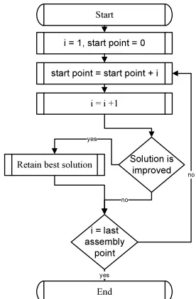
3.4.4.Start point changing

ISSN: www.jatit.org E-ISSN:

much costly, the steps of this procedure is shown in details in Figure 7.

Figure 7: Flow Chart of the Changing Start Point Heuristic

4.RESULT

The SA performance was evaluated using the PCB data in (Leu et al. 1993). The example has 50 components with 10 different component types. The details of the components such as the coordinates of the placement positions and the parameters of the assembly machine (speed of movement of the table, assembly heads and indexing time of the turret) are summarized in Table 1, and have been repeatedly used by others to benchmark their proposed algorithms (Leu et al. 1993; Nelson & Wille 1995; Ong & Tan 2002; Ang et al. 2009; Ho & Ji 2009). Moreover the parameters of SA for the problem are preset as: iteration number=1200, absolute temperature = 0.9999, cooling rate = 0.9888 and temperature =60.

Table 1. The Preset Parameters of the CS Machine

Number of components 50

Number of feeders 10

Number of turret heads 2

Indexing time of turret 0.25s/index Average PCB mounting table speed 60mm/s Average feeder system speed 60mm/s Distance between feeders 15mm

Since the approach used in this study is the iterative approach, which is based on tackling one of the problems in advance followed by the second problem, however changing the priority of the first solved problem needed to be performed to determine the best problem to start the algorithm with, due to this situation of two experiments are conducted to determine whether the algorithm best starts to solve the components assembly problem followed by feeder assignments, or vice versa. The result of the comparison between the two experiments is shown in Figure 8. The figure has been drawn based on 50 runs of SA, showing the best assembly time obtained during each run, the result of solving the components sequencing at first (C1) is shown by the blue dotted line followed then by the feeder assignments. The red squares line showing the situation of solving the feeder assignments problem first (F1) followed by components sequencing,

The graph clearly shown that in the case where the feeder assignment problem is solved first the solution is obtained is better compared to the other situation. This may be due to the fact that the feeder assignment problem is much more difficult than the components sequencing, and the components sequencing problem is dependent to a high degree on the feeder assignments.

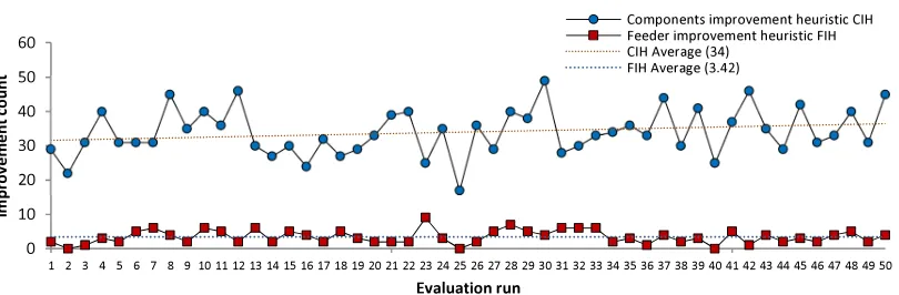
A further investigation is performed to determine the behavior of each experiments where the priorities is changed and to determine the drawback of each case, the measurement is made based on how many times the solution is improved during each experiments of each priority situation; the components sequencing problem when its first solved and the feeder assignments when its first solved. Figure 9 shows the number of solution improvement when the components sequencing problem is solved first. The plots indicate that the feeder assignments improvement counts is very low, and some of the runs have no feeder improvement at all (see the squares dotted line). Moreover, the average of the feeder assignments solution improvement counts is 3.42 among all runs, while the average of the components sequencing improvement solution counts is very high (see the circle dotted line) with 34, compared to the feeder assignments improvement counts.

Referring to Figure 10, the experiment shows a performance balanced between the improvement times of the two problems, in case of solving the feeder assignments first followed by components assembly. Furthermore, this case can be seen as

Start

start point = start point + i

i = i +1 i = 1, start point = 0

i = last assembly

point

End

Solution is improved Retain best solution

yes

no yes

ISSN: www.jatit.org E-ISSN:

similar to the integrated approach, which has been reported using other metaheuristic in several studies, where the aim of the integrated approach is to find the compatible state between the feeder assignment and the components sequencing problems concurrently rather than sequentially as this experiments showed. The average of the improvement counts of the components sequencing problem and the feeder assignment problem is quite close, with the values of 15.78 and 13.42, respectively. As mentioned earlier the best solution obtained from SA is in the situation with the feeder assignment first solved followed by components assembly.

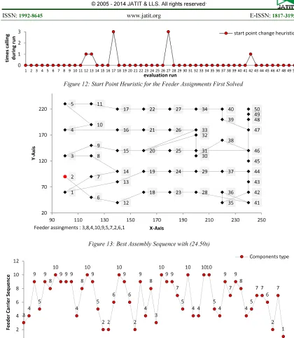
Another experiments is conducted to change the start point after the best solution is obtained, the idea behind changing the start point is due to the fact that using iterative approach where each problem is solved individually rather than concurrently, the components assembly sequences starting point cannot be guaranteed that it's in compatible state with the feeder that is associated with it. An experiment conducted to investigate the proposed technique to determine the effectiveness of changing the start point after the best solution obtained. However a further improvement in assembly time is obtained by 3% and 2.5% for the two cases, the components sequencing first solved and feeder assignments first solved, respectively. The improvement ratio, in seconds, ranged from 0.08 to 0.58 part of a second for the feeder assignments problem first solved, and from 0.8 to 0.67 part of a second for the components sequencing first solved. Figure 11 and 12 provide further details of the heuristic in 50 runs.

4.1.Discussion

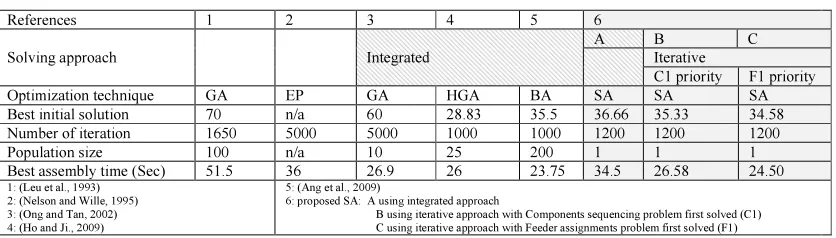
From Table 2, it can be seen that the performance of SA is comparable to that of the other techniques used in (Leu et al. 1993; Nelson & Wille 1995; Ong & Tan 2002; Ang et al. 2009; Ho & Ji 2009), although using different approach which is iterative not integrated approach, it is comparable in three aspects. Firstly, the best solution obtained (24.50s) is among the best reported result and better than HGA by ((Ho & Ji 2009), as can be seen in column C, and less than a second from the best solution so far by (Ang et al. 2009). Secondly, SA can obtain a better solution with one solution as it is a single based metaheuristic, while the other techniques are population based. Lastly, SA can obtain a better

solution not only with a one population, but also compatible with iterations, 1200 versus 1000. However, the experiments show that performance of SA using integrated approach is not as good as using the iterative approach. Referring to column A of the table, it can be said that the nature of single based solution metaheuristic has more chance of being trapped in local optima by using iterative approach, because the components scheduling problem are divided into two problems. Meanwhile the population based which uses multiple agent solution is better in escaping the local optima. Details of best solution obtained by SA are demonstrated using several figures. Figure 13 shows the best solution obtained by HGA, Figure 14 shows the components sequence for the best solution obtained and Figure 15 shows the delay of the three moving mechanisms.

5.CONCLUSION

A Simulated Annealing algorithm incorporated with three different heuristics was applied successfully to the PCB components sequencing problem for chip shooter machines, which is a combinatorial problem of components sequencing and feeder arrangement with the objective of minimizing the total assembly time. The three heuristics are the nearest-neighbor heuristic in initialization, the 2-opt local search heuristic, move heuristic and iterated move heuristic for improvements. Finally, it has been shown that the effectiveness as well as performance of SA has reached that of the other techniques such as HGA and BA in terms of the total assembly time. SA is capable to solve the problem optimally near with almost equivalent results. SA has more areas for enhancement such as improvement with a good search technique. This research has proved that an iterative approach is able to obtain good results similar to the ability of an integrated approach, even though many researchers reported that the iterative approach is not the best way to optimize the CS machine performance, because it cannot guarantee that the solution is globally optimal.

REFERENCES

[1] Ang, M. C., D. T. Pham & K. W. Ng 2009. Application of the Bees Algorithm with TRIZ-inspired operators for PCB assembly planning. Proceedings of 5th Virtual International

ISSN: www.jatit.org E-ISSN:

Machines and Systems (IPROMS2006), hlm.

454-459.

[2] Ayob, M. & G. Kendall 2005. A Triple objective function with a Chebychev dynamic pick-and-place point specification approach to optimise the surface mount placement machine. European Journal of Operational Research 164(2005): 609–626.

[3] Ayob, M. & G. Kendall 2008. A survey of surface mount device placement machine optimisation: Machine classification. European

Journal of Operational Research 186(2008):

893–914.

[4] Crama, Y., O. E. Flippo, J. Klundert & F. C. R. Spieksma 1997. The Assembly of Printed Circuit Boards: A Case with Multiple Machines and Multiple Board Types.

European Journal of Operational Research 98:

pp. 457-472.

[5] Duman, E. 1998. Optimization issues in automated assembly of printed circuit boards.Tesis PhD thesis Bogazici University, [6] Duman, E. 2005. Modelling the operations of a

component placement machine with rotational turret and stationary component magazine.

Journal of the Operational Research Society(0):

1 9.

[7] Ho, W. & P. Ji 2006. A Genetic Algorithm Approach to optimize component placement and retrival sequence for chip shooter

machines. Springer-Verlag Advance

Manufacturing technology(28): 556-560. [8] Ho, W. & P. Ji. 2007. Optimal Production

Planning for PCB Assembly. P. D.T. Ed. London: Springer: Series in Advanced manufacturing.

[9] Ho, W. & P. Ji 2009. Integrated Component Scheduling Models for Chip Shooter Machines. International Journal ProductionEconomics 123: 31-41.

[10]Kirkpatrick, S., C. D. Gelatt & M. P. Vecchi 1983. Optimization by Simulated Annealing.

Science 220(4598): 671-680.

[11]Leu, M. C., H. Wong & Z. Ji 1993. Planning of component placement/insertion sequence and feeder setup in PCB assembly using genetic algorithm. ASME Journal of Electronic

Packaging 115: pp. 424-432.

[12]Moyer, L. K. & S. M. Gupta 1997. An Efficient Assembly Sequencing Heuristic for Printed Circuit Boards Configurations. Journal

of Electronics Manufacturing 7(2): pp.

143-160.

[13]Nelson, K. M. & L. T. Wille. 1995. Comparative Study of Heuristics for Optimal Printed Circuit Board Assembly. F. Lauderdale. Ed. FL, USA: Proc Southcon.

[14]Ong, N. & W. C. Tan 2002. Sequence placement planning for high speed PCB assembly machine. Integrated Manufacturing

Systems 13(1): pp. 35 - 46.

[15]Soneji, H. & R. C. Sanghvi 2012. Towards the improvement of Cuckoo search algorithm. Information and Communication Technologies

(WICT), 2012 World Congress on, hlm.

ISSN: www.jatit.org E-ISSN:

Figure 8: Best Assembly Time for the Two Problems for50 run

Figure 9: Improvement Counts When the Components Sequencing is First Solved.

Figure 10: The Number of Improvement Counts When the Feeder Assignment is First Solved.

Figure 11: Start Point Heuristic for the Components Sequencing First Solved 22

24 26 28 30 32 34

1 2 3 4 5 6 7 8 9 10 11 12 13 14 15 16 17 18 19 20 21 22 23 24 25 26 27 28 29 30 31 32 33 34 35 36 37 38 39 40 41 42 43 44 45 46 47 48 49 50

A

ss

e

m

b

ly

t

im

e

in

s

e

c

.

Evaluation run

Components At 1st Feeder at 1st C1 Average (29.29) F1 Average (26.1)

0 10 20 30 40 50 60

1 2 3 4 5 6 7 8 9 10 11 12 13 14 15 16 17 18 19 20 21 22 23 24 25 26 27 28 29 30 31 32 33 34 35 36 37 38 39 40 41 42 43 44 45 46 47 48 49 50

im

pr

ov

e

m

e

n

t

co

u

n

t

Evaluation run

Components improvement heuristic CIH Feeder improvement heuristic FIH CIH Average (34)

FIH Average (3.42)

0 5 10 15 20 25 30

1 2 3 4 5 6 7 8 9 10 11 12 13 14 15 16 17 18 19 20 21 22 23 24 25 26 27 28 29 30 31 32 33 34 35 36 37 38 39 40 41 42 43 44 45 46 47 48 49 50

im

pr

ov

e

m

e

nt

count

Evaluation run

Components improvement heuristic CIH Feeder improvement heuristic FIH CIH Average (15.78)

0 1 2 3

1 2 3 4 5 6 7 8 9 10 11 12 13 14 15 16 17 18 19 20 21 22 23 24 25 26 27 28 29 30 31 32 33 34 35 36 37 38 39 40 41 42 43 44 45 46 47 48 49 50

ti

m

e

s

cal

li

n

g

d

u

ri

n

g

r

u

n

evaluation run

ISSN: www.jatit.org E-ISSN:

Figure 12: Start Point Heuristic for the Feeder Assignments First Solved

Figure 13: Best Assembly Sequence with (24.50s)

Figure 14: Best Feeder Sequence with (24.50s) 0

1 2 3

1 2 3 4 5 6 7 8 9 10 11 12 13 14 15 16 17 18 19 20 21 22 23 24 25 26 27 28 29 30 31 32 33 34 35 36 37 38 39 40 41 42 43 44 45 46 47 48 49 50

ti m e s cal li n g d u ri n g r u n evaluation run

start point change heuristic

2

6

12

18 23 28

41 36 35 42 43 44 37 29 24 19 13 1 7 14 8 3 9

15 25 31 46

38 30 32 20 33 26 21 16 4 10

5 11

17 22 27 34 40

39 47 48 50 49 45 20 70 120 170 220

90 110 130 150 170 190 210 230 250

Y

-A

xi

s

X-Axis Feeder assingments : 3,8,4,10,9,5,7,2,6,1

3 4 9 5 9 8 10

9 9 9

4 8

10 9

5

2 2 6 10 9 6 2 9 4 8 3 10

9 9

7

5 10

4 4 10 10 5 4 9 7 9 8 4 5

7 7 6 2 7 1 0 2 4 6 8 10 12

1 2 3 4 5 6 7 8 9 10 11 12 13 14 15 16 17 18 19 20 21 22 23 24 25 26 27 28 29 30 31 32 33 34 35 36 37 38 39 40 41 42 43 44 45 46 47 48 49 50

ISSN: www.jatit.org E-ISSN:

Figure 15: Delays of the Three Mechanisms During Assembly Process (24.50s)

Table 2. Comparison of the SA with the Benchmark Result

References 1 2 3 4 5 6

Solving approach Integrated

A B C

Iterative

C1 priority F1 priority

Optimization technique GA EP GA HGA BA SA SA SA

Best initial solution 70 n/a 60 28.83 35.5 36.66 35.33 34.58

Number of iteration 1650 5000 5000 1000 1000 1200 1200 1200

Population size 100 n/a 10 25 200 1 1 1

Best assembly time (Sec) 51.5 36 26.9 26 23.75 34.5 26.58 24.50

1: (Leu et al., 1993) 2: (Nelson and Wille, 1995) 3: (Ong and Tan, 2002) 4: (Ho and Ji., 2009)

5: (Ang et al., 2009)

6: proposed SA: A using integrated approach

B using iterative approach with Components sequencing problem first solved (C1) C using iterative approach with Feeder assignments problem first solved (F1)

0 0.2 0.4 0.6 0.8 1 1.2 1.4

1 3 5 7 9 11 13 15 17 19 21 23 25 27 29 31 33 35 37 39 41 43 45 47

d

e

lay

t

im

e

i

n

s

e

c

(3

m

ach

an

is

m

)

Placement Sequence

Components assembly delay

Feeder assignments delay