3 4 5h Hybrid Simulation of an Aircraft Adaptive Control System 1963 pdf

[

HYBRID SIMULATION OF AN AIRCRAFT ADAPTIVE CONTROL SYSTEM

by

Peter W. Halbert

Applications Engineer, Electronic Associates, Inc. Princeton, New Jersey

ABSTRACT: Aircqtft adaptive control is simulated in real time by a

hybrid system (HIDAC* 2000) consisting of a general purpose analog computer and parallel digital logic and conversion components. The

proposed adaptive technique utilizes predicted as well as measured past information on aircraft behavior to calculate optimum controller parameters. The optima are determined by a systematic search pro-cedure in parameter space. The search program is under the direction of the logic elements and employs an analog computer model of the

air-craft system, solved at high speeds for prediction purposes. Fast adapta-tion to environmental disturbances is shown to be realizable.

THE ADAPTIVE CONTROL PROBLEM

The general concept of adaptive control has be-come well known. and the objectives and various types of adaptive systems have been classified. 1 In particular, for adaptive control of a high per-formance aircraft, it is desired to alter the feed-back control parameters in the basic linear COntrol system to correct for unknown, unanticipated, or unaccounted-for changes in the aircraft's operating characteristics, inputs, or criterion of peTform-ance.

A typical adaptive scheme to accomplish this pur-pose measures and evaluates the aircraft's per-formance over some recent time interval, makes deCisions regarding any necessary control loop parameter modifications, and implements these Changes.

Of interest is the speed of adaptation. The time required in the adaptive process above (for a rea-sonable quality of adaptation) is usually much longer than the characteristic time constant of the sys-tem. 2 It is suggested here that faster adaptations would obtain if the evaluation of system perform-ance were made on the basis of predicted future

1

aircraft performance as well as measured past performance.

Accordingly, an adaptive scheme is proposed wherein environmental Changes are reflected in

an on-board model of the aircraft control system. The model, in turn, is used to predict future

air-craft performance and, in conjunctAon with an

optimization program, to determine optimum con-troller parameters. Prediction is done via high-speed integration of the model equations; there-fore, optimization is rapid, and a new set of controller parameters can be instituted almost

as soon as a measurement of performance indi-cates a need for Change.

The feasibility of using a predictive technique of this sort is to be determined by means of a

hybrid simulation. Of particular interest is the quality of adaptation, i.e. the magnitude of de-partures from optimum performance in the face of environmental upsets. Since a hybrid approach

is applicable to problems requiring both logical calculations and high-speed iterative solution of differential equations, its use is justified in this problem, where these requirements are imposed by the optimization technique.

THE HYBRID SYSTEM

One of the major forms of hybrid computation to emerge in recent years is the association of a general purpose analog computer with a comple-ment of general purpose digital logic, memory, and conversion components. The genesis of this type of computational system began with a desire to exploit the high"':speed integration capability of the analog computer. The consequent need to con-trol and Change the analog's program on the basis of previous results and external inputs and at cor-respondingly high speed led to the adoption of the parallel digital devices, programmed to exercise the necessary logical control, timing, and data

storage functions.

Applications of this type of hybrid computation include iterative calculations, automatic production of a sequence of analog runs, and solutions of partial differential equations via techniques re-quiring function storage and iteration. 6 The addi-tional capabilities of this system to perform auto-matic optimization of system parameters and to simulate systems containing digital devices are of interest in this problem.

The adaptive control problem imposes computa-tional requirements of two- speed integration of the system equations with iterations of the high-speed solution under direction of the digital logic

elem~nts. These latter are also programmed to automatically test the results of analog iterations, make logical decisions from evaluations of these results, and execute commands aimed at deter-.mining optimum system parameters. The analog

computer provides the simulation of the aircraft and control system, their models, and also of a dynamic reference model which provides a criterion for evaluating system performance. The parallel digital elements, in addition to their role in direct-ing the optimization, are programmed to act as master control of the entire simulation. With the exception of the representation of the actual air-craft and control system, the simulation is re-garded as one of a potential on-board adaptive control system. The simulation itself is considered to be representative of those in which the full speed capability of the analog computer is utilized.

THE OVERALL ADAPTIVE CONTROL SYSTEM

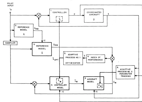
The elements essential to the adaptive technique are shown in Figure 1 and comprise:

1. an Aircraft Control System whose feed-back control parameters

'X

(vector nomen-clature) are the objects of adaptation.

2. a Performance Criterion in the form of a dynamic reference model (with parameters "'ij), arbitrarily specified but known to

pro-duce a desirable response xRM(t) to pilot inputs ~ (t) •

3. Auxiliary Models (heavy black boxes in Figure 1), having parameters ~ M, PM' and

q,

corresponding to actual system parameters, to be used to calculate (via high- speed integration) the predicted re-sponses xM(t) and xRM(t) for use in the optimization program.

4. a Predicted Index of Performance, E, de-fined by

E

=t+Tl~

-

XM/dt (1)

where T is the prediction interval.

5. Adaptive Process No.1, an automatic optimization program, which computes iJE/

a~M and the optimum

1

_M,

6. Adaptive Process No.2, a parameter tracking program, which calculates opti-mum PM from measurements of actual system performance.

The form of the Performance Criterion and the. use of Auxiliary Models are suggested by the "Model- Reference-Adaptation" technique of Whi-taker3 and an ' 'auxiliary

sy~tem'

, concept of adaptation as discussed by Widro~, respectively. The approach taken here, however, is different from both of these in its utilization of high- speed prediction.

The predictive technique operates as follows. Adaptive Process No.1:

1. makes small perturbations in A Mi (each component. of). M) •

2. measures E over a prediction interval with the perturbed AMi"

3. calculates

a.E/

aXM

(approximately) •

.. :.1': ...

4. alters A M so that E will be reduced.

PILOT INPUT

ip

I.

( CONTROLLER COORDINATED

U _{--. AIRCRAFT} X

-

_r--'

-A

L

>.J

Ii

2.

REFERENCE iRM

r----

MODEL q

•• IC

l

SAMPLER

1

3. _iRM

REFERENCE MODEL

q 5.

ADAPTIVE

n

4. INDEX OF ~OPT r-- PROCESS NO. I:

PERFORMANCE

OPTIMIZATION

6. _~

ADAPTIVE PROCESS NO. 2

PARAMETER TRACKING +-

-r-= .,

_-

3. AIRCRAFT

-r

_{L_~} AM I uM MODEL _xM

3. CONTROLLER

r- ,

LPM1

MODEL _:.J

IC A~ IC

Figure 1: Adaptive Control Scheme

By itselft adaptive loop no. 1 does not provide complete adaptive control. A second adaptive process is necessary to track the parameters PMt updating the predictive model in an attempt to match aircraft performance. Thus, variations in the operating characteristics or inputs to the actual aircraft occur as parameter changes in the aircraft modelt the objective being to alter or force the predictive loop to imitate the actual air-craft as closely aspossible. The effects of environ-mental perturbations also appear in the auxiliary model via the transfer of information on the cur-rent statet

x

and

u

_{t of the aircraft and its feedback} control system. This information is used as initial conditions in the iterative prediction calculations. In summary, adjustment o~

PM

allows prediction and henCe optimization of A M on the basis of the current estimate of the aircraft transfer function; and state variable transfer permits prediction from the correct current state.

It should be evident from the above that the deter-mination of the optimum ~ by calculation of

aE/

a

iM

presumes the constancy of parameters

'PM

and

q,

pllot input ~, and state variables

x

and IT

over the prediction interval T. Since this condition does not necessarily prevail due to changing en-vironmental conditions, unpredictable pilot be-haviort or changing performance criteriat it is necessary to constantly re-evaluate

a

E/

a

~M and the optimum

X •

This is a reasonably simple task

~n the sys::'em at hand, since

PM

(t),

q

(t), Ip (t), x (t)t and u (t) will presumably be low-frequency functions and essentially constant during a few

[image:3.618.66.561.49.403.2]

Other non-predictive adaptive schemes are, of course, faced with similar problems of current "optima" lagging the true optima. This is due to the time lag between the measurement of perform-ance and implementation of correction. 3 Generally these schemes have much longer lag times than the predictive techniques. Note for comparison pur-poses that both adaptive processes of Figure 1

operate very rapidly so that corrective action can begin essentially as soon as environmental per-turbations become evident in the aircraft outputs. This delay is determined by various aircraft system time constants and the nature of the per-turbations.

Although corrective action is fast, the quality of adaptation may be suspect if predicted response differs significantly with actual future perform-ance, or if repeated evaluations of the optima are ineffectual in producing necessary corrections. Such situations can conceivably exist when:

1. the aircraft model and actual aircraft are described by significantly different transfer functions, and the mismatch cannot be com-pensated by parameter tracking.

2. parameter tracking and state variable transfer is ineffectual in transferring to the model sufficient information on the nature of the actual disturbance.

3. ~ and PM vary drastically over the pre-diction interval.

The consequence of 3. above is evident upon con-sideration of ip (t). Values of this function are sampled at the start of each prediction calcula-tion and assumed to prevail over the entire pre-diction interval. It is true however that the

-

"

optimum A depends not only on the present value of ip (t) but on its functional nature as well. To as-sume a form for the function, namely ip (t)

=

con-stant, even though the constant is updated from prediction to prediction, may lead to an inaccurate calculation of the optimum. This situation may be overcome by extrapolating the recent past history of ip (t) over the prediction interval. Such a modi-fication would allow for greater utilization of pre-sent information in predicting future performance.

The ip sampler at the input to the auxiliary sys-tem now has a dual purpose. It prevents discon-tinuous plIot inputs from affecting the prediction during the course of a run (pilot inputs are re-garded here as being piecewise continuous with low frequency content over continuous segments), and it becomes part of the extrapolation system.

AIRCRAFT CONTROL SYSTEM AND MODELS

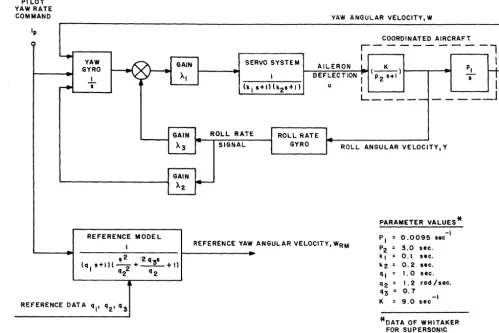
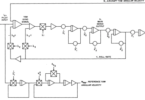
A yaw control system for a supersonic transport (Figure 2) as presented by Whitaker4, was chosen to demonstrate the adaptive technique.

The aircraft control system is expected to perform satisfactorily over extremely wide ranges of speed and altitude. The attendant changes in perform-ance characteristics and a variety of environ-mental conditions make modification of the con-troller gains necessary. In the system the pilot's input yaw rate is monitored by a yaw integrating gyro which produces a control action causing the vehicle to roll until a component of its angular velocity about its yaw axis is equal to the yaw rate command. (More detailed descriptions of this system are given in reference 3.) The same basic fifth-order representation was used for both the actual aircraft control system and its model, although nonlinearities and additional inputs were frequently included in the actual system in order to test the adaptive scheme.

Three control loop gains are to be adjusted: AI' A 2, A 3, corresponding to gains in the forward loop, the roll angle stabilization loop, and the roll rate damping loop, respectively.

The reference model is seen to be a third-order system with three parameters, ql' q2' q3, which are time constant, frequency, and damping factor, respectively. These parameters define the desired response and may be altered at will.

A single aircraft output, the yaw angular velocity,

W, is taken as a measure of aircraft performance. It is assumed that delays in measuring all output variables are negligible.

INDEX OF PERFORMANCE

A single index of performance given by E

=

{t+ T

I

W RM - W

I

dt was used to adjust the three

parameters. This was later found not to be opti-mum due to the existence of local minima, in-sensitivity to certain parameter changes, and parameter cross-coupling, but is retained here for the sake of exposition of the technique. A better approach employs several E's defined by:

t+1'

Ei =

f

2i W _{RM - W} d _{t i}

₌

_1,2,3

t+Tli

(2)

PI LOT YAW RATE

COMMAND YAW ANGULAR VELOCITY, W

YAW GYRO

COORDINATED AIRCRAFT

r - - - l

SERVO SYSTEM AILERON I I

I--~"..,....",...,...~"" t _K_ ) PI .L

s

ROLL RATE

SIGNAL

DEFLECTION I P₂ &+1 S

I

_____

J

U I L-... _ _ ' "

L _ _ _ _

ROLL ANGULAR VELOCITY, Y

PARAMETER VALUES*

REFERENCE MODE L

I REFERENCE YAW ANGUL.AR VELOCITY, WRM

-I

P I = 0.0095 sec

P2 = 3.0 sec. kl = O.l sec.

k 2 = 0.2 sec.

q I = I. 0 sec. q 2 = I . 2 rod / sec.

q3 = 0.7 _I K = 9.0 sec

*DATA OF WHITAKER FOR SUPERSONIC TRANSPORT.

M = 3.5 @ 75,000 FT.

Figure 2: Aircraft Control System Block Diagram 4 (Form of System and Parameter Values According to Whitaker)

ADAPTIVE PROCESS NO.1

The optimization technique used is a modifica-tion of the method of steepest descents according to Witsenhausen5• A search to find the minimum of E (AMI, AM2, AM3) from an arbitrary initial starting point AOMl' AOM2, AOM3 and EO proceeds as follows:

1. By perturbing the AMi values by a small amount h calculate approximate partial derivatives

(3)

where

bE+ = E (AMl' "',

A~H

+ h, "',

A~3)

- EO

(5E = E (AMl' "', A~i - h, ''', A~3) - EO

This requires six high- speed prediction runs.

2. Store the results of all partial derivative determinations. This is done in quantized form to place the storage load on the digital computer. The quantization is done by comparing the partial derivatives with a quantity L, arbitrarily but carefully specified, and determining a new quantity Zi:

Zi =+ 1, (5E+ - (5E-)

< -

2hL

+

-n, -

2hL «aE -

oE )

<

2hL (4)

+

-= -

1, (0 E - (5 E )

>

2hL

The unit vector Z defines a direction in A-space in which a decrease in E is probable.

3. Adjust the parameters to AM. + Z. A, where A is some fixed quantity.1 1

[image:5.626.58.557.62.395.2]

with a smaller ~. When this also fails, repeat the whole process starting from the new position in AM space.

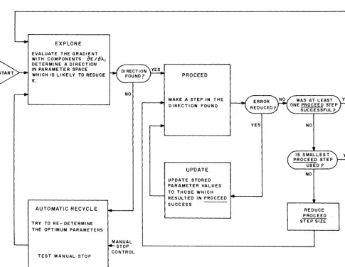
5. Stop the optimization procedure when either all Zi == 0 or when at least one improve-ment cannot be obtained with the smaller ~ proceed steps,

The information flow for this procedure is given in Figure 3. Note the automatic recycle feature provided to continuously re-evaluate the optimum following its initial determination. The recycle is started automatically following a stop condition, provided that a manual stop command has not been issued by the operator, It is very important upon recycling to re-evaluate the reference error EO by making a run with the A i currently in effect. Failure to do so may result in a "locked-in" condition, wherein a new optimum cannot be achieved because the new minimum E is greater than the EO just determined. Such a condition can

~ _EXPLORE

EVALUATE THE GRADIENT

~

WITH COMPONENTS DETERMINE A DIRECTION OE/OAj

IN PARAMETER SPACE

f-fIRECTIO~

WHICH IS LIKELY TO REDUCE _FOUND? E.

,---II' NO

----...

'

-AUTOMATIC RECYCLE

TRY TO RE- DETERMINE THE OPTIMUM PARAMETERS

' - - - ~ANUAL _STOP

CONTROL TEST MANUAL STOP

occur because environmental upsets in effect "shift" the E hypersurface.

Refinements in the basic program, as suggested in Reference 5, were made in order to decrease convergence time.

ADAPTIVE PROCESS NO.2

The actual aircraft can be described by some vector function of the form

(5)

where

r

refers to environmental inputs. The air-craft model is defined by

(6)

We seek the values for

PM

for which the actual system outputs and model outputs coincide as well as possible. This optimum is obtained directly by

PROCEED

MAKE A STEP IN THE

KERROR

NO WAS AT LEAST YES DIRECTION FOUND _REDUCED? ONE PROCEED STEP

SUCCESSFUL? YES NO

t

IS SMALLEST~ PROCEED STEP

UPDATE

USED? NO UPDATE STORED

PARAMETER VALUES TO THOSE WHICH

RESULTED IN PROCEED _~ SUCCESS

REDUCE PROCEED STEP SIZE

[image:6.631.49.535.327.703.2]

substituting

x

=x_M, U =u_M, and~ =~M into equation (6) and solving the resulting algebraic expression for PM- This technique is valid if the number of components of PM are eq~al to or less than the number of components of ~M' It also is based on the assumption that the necessary state variables and control variables can be measured. It may be necessary to differentiate (and filter) aircraft outputs to obtain certain components of

1.

It is of interest to note that differences between the actual aircraft and its model

{r

1=

~ or the existence of environmental inputs

(I

1=

zero) are reflected in the model via changes in PM'

For the system under consideration equation (6) is

•

WM=PMlYM

(7)

• 1

Y = - ( K u - Y )

M PM2 M M M

where KM is taken to be constant. The optimum PMl are given by

•

PMl = W/Y

PM2 = (K_M u -

y)/Y

(8)

A difficulty in determining these quotients occurs under steady state conditions, when numerators and denominators become zero but PMl and PM2 are determinate. A division circuit using the method of steepest descents 7 affords a solution to the problem and was used in the simulation. Initial values for PMl and PM2 were obtained from a knowledge of Pl and P2 under assumptions that

f

=

g

and 1=0 initially.

The roll rate Y is measured by a roll rate gyro as part of the basic control system. Wand

Y

would have to be determined by differentiation of aircraft outputs Wand Y. The main servo output u could be measured easily.

Other, more sophisticated parameter tracking techniques could be used. 8 The possibility of time- sharing the optimization techniques of Adap-tive Loop No. 1 was also considered. These alter-natives are feaSible, but require considerable addi-tional computation. The technique used provided satisfactory results with a modest expenditure of computational equipment.

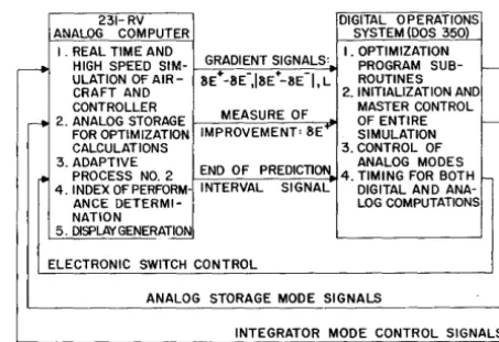
ALLOCATION OF TASKS IN THE HYBRID PROGRAM

The hybrid system was an Electronic Associates HYDAC 2000computerconsistingofaPACE® 231-R

general purpose analog computer and a digital operations system (DOS 350). The 23l-R was equipped with a high- speed electronic mode con-trol unit (MLG). The allocation of computational tasks are shown in Figure 4.

231-RV DIGITAL OPERATIONS ANALOG COMPUTER SYSTEM (DOS 350)

I . REAL TIME AND

GRADIENT SIGNALS: I. OPTIMIZATION

,..- HIGH SPEED SIM- PROGRAM SUB-

r--ULATION OF AIR- SE+-SE-.lsE+-8E-I. L ROUTINES CRAFT AND 2. INITIALIZATION AND CONTROLLER

MEASURE OF MASTER CONTROL

,.

2. ANALOG STORAGE OF ENTIRE I

-FOR OPTIMIZATION IMPROVEMENT,BE+' SIMULATION CALCULATIONS 3. CONTROL OF 3. ADAPTIVE ANALOG MODES

r

PROCESS NO.2 ENO OF PREDICTION 4. TIMING FOR BOTH I

4. INDEX OF PERFORM- INTERVAL SIGNAL DIGITAL AND ANA-ANCE DETERMI- LOG COMPUTATIONS NATION

~5~~ERA~

ELECTRONIC SWITCH CONTROL

ANALOG STORAGE MODE SIGNALS

INTEGRATOR MODE CONTROL SIGNALS

Figure 4: Allocation of Computer Tasks

THE ANALOG PROGRAM

An unscaled schematic for the basic aircraft sys-tem is given in Figure 5. Two of these circuits are required, one operating in real time to repre-sent the actual system, the other at high speed (1000 times faster) for prediction. Noise inputs, failure conditions, and changes in the structure of the circuit were applied only to the real time cir-cuit. The parameters Pl and P2 were fixed in the actual system circuit, but variable (as determined by the tracking process) in the predictive circuit. Initial conditions for the actual system were taken to be zero; the initial conditions for integrators in the predictive circuit were taken from outputs of their corresponding real time integrators. The parameters

X

M and ~ were determined for the two cirCuits by different logic programs: the>' M were modified to evaluate

aE/aA

M

but Ai were changed only if predictlon with A °Mi + Zi ~yielded a sma~ler E. (Note that AM' is equivalent to A,.)

1 1

Proper scaling of the gains A M' and A, was

es-. 1 1

sential for the optimization process. Use of a single, fixed exploration step size, h, depends on this. Improper scaling results in a gain between a E/a A Mi and A Mi that is either too high or too low, causing the optimization to stop at a non-optimum point or produce unstable solutions. A few simple trial-and-error experiments on the computer permitted determination of appropriate scale factors.

[image:7.621.336.563.139.294.2]

calcu-i p, PILOT INPUT

W, AIRCRAFT YAW ANGULAR VELOCITY

Y, ROLL RATE

W_RM, REFERENCE YAW

ANGULAR VELOCITY

Figure 5: Analog Circuit for Aircraft, Controller, and Reference Model (Unscaled)

late PM1 and PM2 according ~o equati~n (8). In the simulation the derivatives Wand Y appear as explicit voltages and need not be determined by differentiation.

THE DOS PROGRAM

The DOS consists of a collection of programma-ble, parallel digital logic, memory, and conversion components. Only the logic and some conversion components were used in this problem. These include logic gates, clocked flip-flops, shift reg-isters, mono stables , counters, comparators, and electronic switches, which can be interconnected on a patch panel in a manner similar to analog computer programming. Propositional and se-quential logic calculations are handled by the gates and flip-flops, respectively, or by packaged combinations of these (shift registers, counters, etc.), The comparators and electronic switches provide the analog-to-Iogic and logic-to-analog conversions. In addition, logic levels on the DOS can control electronic switches in the analog cir-cuits, the modes of analog integrators, and the

modes of track-hold analog storage units. The operating details of these devices as well as their program symbols are considered elsewhere. 5,6&9

In this simulation the DOS directs the entire optim-ization program. The mechanoptim-ization of the pro-gram, including circuit diagrams, has been given by Witsenhausen. 5 It suffices here to note the program structure-a set of subroutines, appro-priately interlocked, whose functions are to:

1. select the step sizes h, ~ 1, and ~2 and set the appropriate switches accordingly. (See Figure 6.)

2. test for stop - recycle conditions.

3, initiate a high speed analog run to deter-mine E, with a single parameter aug-mented by + h, then -h, repeating this for all three parameters.

[image:8.624.57.541.64.398.2]

5. initiate a high- speed analog run with the appropriate Zi ~ modifications in all three parameters and test for improvement.

6. update the A i and EO analog storage units to the values of A Mi and E that resulted in improvement.

7. repeat steps 5 and 6 until no improve-ment is obtained or until a preset num-ber of "proceed" steps have occurred.

8. repeat steps 3 - 7 until a stop - recycle condition occurs.

9. clear the results of previous logic cal-culations when a stop - recycle condition exists, make another analog run with the present A Mi' and store the resulting value of E as the new EO; start with step 1 again.

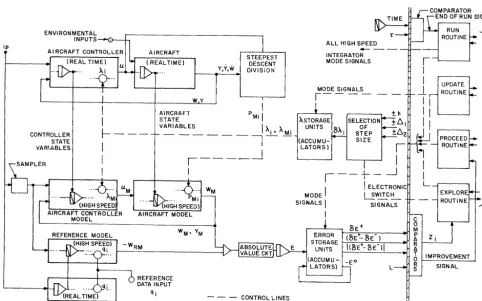
The hybrid program is shown schematically in Figure 6 with emphasis placed on the interface. Various portions of the analog program are repre-sented symbolically by a single integrator; param-eters are represented by a potentiometer symbol. High- speed portions of the program are indicated by a slash line drawn through the integrator

sym-ip

ENVIRONMENTAL

INPUTS~:·)--+.

CONTROLLER STATE VARIABLES

I

I

~---I

I

I

Y,Y,W

bol. The storage units employed analog integra-tors, programmed as accumulators. Selection of the magnitude and sign of the A perturbations (c) Ai) was done by electronic switches under con-trol of the DOS logic elements. Concon-trol outputs of the DOS subroutines are indicated; their inter-connections are given in reference 5.

RESULTS

Responses of the adaptive control system to a variety of test conditions are presented in Fig-ures 7 - 11. The standard aircraft and reference model parameters given in Figure 2 were used unless otherwise specified.

Convergence: Figures 7a and 7b illustrate the speed of convergence to an optimum state from an arbitrary initial set of parameter values. The optimization procedure brought the parameter values for AI, A2, and A3 from 60, 10 and 20 (dimensionless as shown in Figure 7b), respec-tively, to 70, 18, and 11 in approximately 1.2 seconds. The index of performance E was reduced to 5.0% of its original value. The input function was a series of steps applied by the pilot in an attempt to perform roll-in and roll-out maneuvers. Although a perfect correspondence between actual

STEEPEST DESCENT DIVISION

---INTEGRATOR MODE SIGNALS MODE SIGNALS

r-~--ASTORAGE SELECTION UNITS 8Aj S~~P (ACCUMU- SIZE

LATORS) ,

I

,--+-_-.J

I

\

ELECTRONIC MODE ~WITC~

SIGNALS \ SIGNALS

I

L

I I

I ~

II

1\

II

:LJ

-,

\

I

L

SIGNAL

V)

w z

i=

::>

o 0:: II:: W

J:

I-o

~

o II:: LL

o

I-- - - CONTROL LINES REFERENCE MODEL - - - DATA LINES

[image:9.627.65.547.406.706.2]

A B C

I

5 10

A = REFERENCE MODEL RESPONSE B = AIRCRAFT RESPONSE C= AIRCRAFT RESPONSE

WITH-OUT ADAPTIVE CONTROL

I

A B C

15 40

TIME, SECONDS

45

Figure 7a: Aircraft Response to Pilot Inputs. Con-troller Gains Initially Non-Optimum

15

>'1

10

5

...J

cr tL.

~ ~o~ __ ~~ ____ L-_T~I~M~E,~S~E~C~ON~D~SL-________ ~~

~ ...c 0.5 1.0 1.5

...c .!c

-5

-10

-15

Figure 7b: Adaptation of Gains During a Portion of Response of Figure 7 a

and reference model responses was not obtained, the actual response was a drastic improvement over the marginally stable response that would have obtained in the absence of adaptation. Note also that the marginally stable solution is the first response obtained in the iterative optimiza-tion program, and the final response is the one

shown for the actual aircraft. Approximately 40 high speed prediction runs were made in the inter-vening 1.2 second period. The prediction was made with T = 20 seconds (real time), correspond-ing to 20 ms of computational time in the high speed loop. The speed of adaptation is seen to be so rapid that actual performance is scarcely af-fected by the poor initial values of A. It was as-sumed in this experiment that Pi = PMi and that no environmental effects were operative. The speed of adaptation found here is considerably faster than that reported by Whitaker for essentially the

same aircraft control system but different adaptive technique.

Environmental Effects: Using a slightly altered reference model (ql =1.25), the response to a change in the aircraft's operating characteristics was ob-tained. At time t = 0 events occurred within the aircraft leading to a step change in velocity (in-crease). This change is sensed by Adaptive Process No. 2 in the manner shown in Figure 8a, i.e. PMl changes. Without this parameter adjustment a poor response would result (curve C). With no adaptive control operating at all a poorer response obtains (not shown).

6

.:1

A=REFERENCE MODEL RESPONSE B= AIRCRAFT RESPONSE C= RESPONSE WITHOUT ADAPTIVE LOOP NO.2

a WITH ).'S OPTI-MUM FOR AIRCRAFT BEFORE ITS CHAR-ACTERISTICS CHANGED

8 10 12 14. 16 18 20 22 24 TIME, SECONDS

.01~2

4

f~ .008 ______________________________ __

[image:10.626.37.300.57.215.2]

.006

Figure 8a: Aircraft Response to Pilot Inputs. A Change in Aircraft Speed @ '1=0 Initiates Adaptation

8

4

...J

cr

E

tL. Z _~o

-< -< I 4 8 I

~

-<

-4

TIME. SECONDS

-8

Figure 8b: Gain Adjustments During Response of Figure 8a

The response to an unanticipated input to the air-craft, in the form of a large, constantly applied deflection of the control surface, is shown in Figure 9. This was a most severe test of the adaptive system and demonstrated the need for improvement in defining an index of perform-ance. Parameter cross-coupling with the present E was significant in this experiment. It is felt that the modifications suggested above would

[image:10.626.308.547.224.561.2] [image:10.626.54.279.266.467.2]

c

W N

CONTROL SURFACE MALFUNCTION

@t .0 NORMAL CONTROL " / C ACTION,RESTORED

r

~

./'""..

~

: A -REFERENCE MODEL '/ ' - " - - " , . . . . - - - - " " " : \ RESPONSE

:i

c( ... A

~ 1.0 -~'\---....

l B . AIRCRAFT RESPONSE C -AIRCRAFT RESPONSE WITH NO ADAPTIVE CONTROL

~ PILOT INPUT COMMAND

o ~-...L.-_--.l-_----' _ _ ...l---l_lj ~

o 10 20 30 40 50 ~60 70 80

TI ME. SECONDS

Figure 9: Aircraft Response to Pilot Inputs. Adap-tation Initiated by Control Surface Mal-function

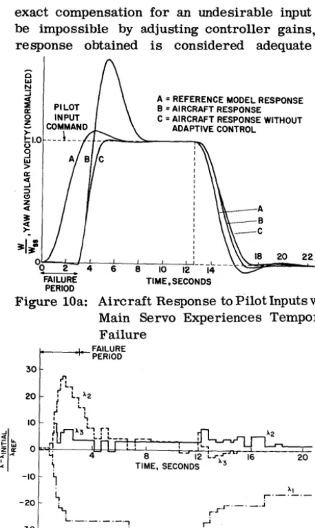
exact compensation for an undesirable input may be impossible by adjusting controller gains, the response obtained is considered adequate and

a _L&J

N :J

of A = REFERENCE MODEL RESPONSE

~ PI LOT B = AI RCRAFT RESPONSE

~ COI~~,UATND C = AIRCRAFT RESPONSE WITHOUT

mm ADAPTIVE CONTROL

~1.0 __ J ___ - -",.-_-.-,;: _ _ _ ~

o

d

> IX:

of

...J

;:)

(!)

z

of

~

of

>-30

20

-10

-20

-30

-40

20 22 ~~-J-+-6~~8--::10~~12

--'4 ---\:

,~,-=--"""

TIME,SECONDS

Aircraft Response to Pilot Inputs when Main Servo Experiences Temporary Failure

1---t<o-~~IMb~E

~

r·-~·-i"

r·r.r· - . _ . j

i..._._._._., ~

~ _{L...._._._."-"'\...j} ~

Figure lOb: Gain Adjustments Under Conditions of Temporary Servo Failure

certainly better than that obtained without adap-tive control.

The response to a failure condition is shown in Figure 10. At time t =0, the main servo becomes "locked" in an inactive state and remains in this condition for three seconds. This is an "open-circuit" type of failure. During the three second period the remainder of the control system, which operates correctly, reaches some limit condition, because no feedback signals from the aircraft outputs are forthcoming. At t = 3, the servo opera-tion becomes normal. The response of the system from the limit condition then reached is of interest. Adaptive control is seen to institute corrective action very rapidly and avoids the large over-shoot associated with no adaptive action.

Changing Goals: Intentional changes in theparam-eters qi, should lead to new aircraft perform-ance, since the reference model is now changed. The successful adaptation to these changing speci-fications is shown in Figure 11.

TIME.

A=AIRCRAFT RESPONSE B = REFERENCE MODEL

RESPONSE DASHED CURVE IS REF-ERENCE MODEL RE-A SPONSE THRE-AT WOULD

[image:11.629.80.336.58.727.2]

HAVE OCCURRED IF REFERENCE PARAME-TERs HAD NOT CHANGED AT T=O. THE GAINS AT T=O WERE OPTIMUM FOR THIS RESPONSE. 16 18

Figure 11: Aircraft Response to Pilot Inputs. Ref-erence Model Changes During Man-euvers

CONCLUSIONS

[image:11.629.88.310.66.265.2] [image:11.629.75.304.324.708.2] [image:11.629.342.573.363.527.2]

REFERENCES

1. Eveleigh. V.W •• "Adaptive Control Systems". Electro-Technology, April, 1963.

2. Wldrow, B .. "The Speed of Adaptation In Adaptive Control Systems", ARS Guidance, Control, and Navigation Conference, Stanford, California, August, 1961.

3. Whitaker, H.P., Yamron, J., and Kezer, A., "Dp-slgn of Model-Reference-Adaptive Control Systems for Aircraft", Report R-I64, Instrwnentation Laboratory, Massachusetts Institute of Technology, September, 1958.

4. Whitaker, H.P .. Kezer, A., "Use of Model-Reference-Adaptive Systems to Improve Reliability", ARS Guidance, Control, and NaVigation Conference, stanford, California, August, 1961.

5. Wltsenhausen. H.S., "Hybrid Techniques Applied to OptimlzationProblems", Spring Joint Compuler Conference, San Francisco, California, May, 1962.

6. Wltsenhausen, H.S .. Landauer, J.P., et.al, "Applications Reference Library on Hybrid Computation", Electronic Associates Inc., Princeton, New Jersey.

7. Favreau, R. R., "Dividing Circuit Obtained by Applying Method of steepest Ascents", PCC Report No. 132, Electronic ASSOCiates, Inc., Princeton, New Jersey.

8. Purl, N.N., Weygandt, C.N., "Multivartable Adaptive Control System", IEEE Transactions, May, 1963.

9. Halbert, P.W., Landauer, J.P., and Wltsenhausen, H.S., "Hybrid Simula-tion of Adaptive Path Control", AIAA Proceedings of the SimulaSimula-tion for Aerospace Conference, Colwnbus, Ohio, August, 1963.

ACKNOWLEDGMENT

The author gratefully acknowledges the technical assistance and suggestions afforded by Mr. Omri Serlin and Mr. Hans Witsenhausen. In addition, Mr. A. I. Katz, Mr. J. J. Kennedy, and Mr. D. F. Welsher offered helpful comments on this paper.

EAr

ELECTRONIC ASSOCIATES, INC. Long Branch, New Jersey