ISSN: 1992-8645 www.jatit.org E-ISSN: 1817-3195
SPOKEN DOCUMENT CLASSIFICATION BASED ON LSH
ZHANG LEI, XIE SHOUZHI, HE XUEWEN
Information and communication engineering college, Harbin engineering university
Harbin, Heilongjiang, China
E-mail: [email protected]
ABSTRACT
We present a novel scheme of spoken document classification based on locality sensitive hash because of its ability of solving the approximate near neighbor search in high dimensional spaces. In speech-text conversion stage, although lattice can provide multi-hypothesis during speech recognition, it is too complex to extract proper word information. Confusion network is adopted to improve word recognition rate while keeping the corresponding posterior probability. In vector space model, modified tfidf on posterior probability is proposed to handle the negative effects of the words with very low posterior probability. Furthermore, after generating the indexing structure based on locality sensitive hash, 1-nearest and N-nearest schemes are adopted in classifier. To spare the execution time, fast locality sensitive hash is conducted. Experiments on the data from four kinds of video programs show the effectiveness of proposed scheme.
Keywords: Spoken Document Classification, Local Sensitive Hash, Confusion Network, Lattice.
1. INTRODUCTION
Spoken document classification is an effective approach to manage and index the speech archives. This task concerns to label a pre-defined topic (class) to a spoken document on its contents. There are two main problems in spoken document classification. One is what kind of output form of speech recognition system is adopted, and the other one is how to deal with the problem of high dimension in vector space model (VSM) [1]. Lattice is fully used due to its providing alternative speech transcription hypotheses [2,3]. But from lattice to VSM, it is complex to extract word information. As for high dimensional problem, dimension reduction is normally used, such as LSA [4] and PCA [5]. However, there will be information lost during the dimension reduction. In this work, we proposed to use locality sensitive hash (LSH) [6] to deal with the classification in original high dimensional space.
The main contribution of this work lies in: 1) Applying LSH as a classification approach in spoken document classification system. 2) Adopting the posterior probability in high dimensional space building (VSM). 3) Improving LSH to reduce the execution time while keeping
the classification performance. 4) Employing confusion network to avoid the complex word information extraction in lattice.
The rest paper is organized as follows: in section 2, we give an overview of the whole framework. In VSM building, tfidf based on posterior probability is proposed to handle the negative effects of the words with low probability. Then the details of classification based on LSH are introduced in section 3. From the basic idea of LSH to parameters determining to fast LSH proposing, this part gives how to classify the spoken document based on LSH. In section 4, several experiments are conducted to verify the effectiveness of proposed approach, including comparison between tfidf and modified tfidf, contrast of LSH and KD-tree, and so on. We then give the conclusion based on theory analysis and experiments results.
4 shows empirical evaluation and comparison to other methods.
2. METHODOLOGY
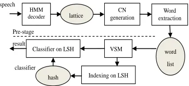
The whole system is shown in Figure. 1. Firstly speech archives are converted into lattices on HMM decoder, which can be done easily based on HTK. Although global utterance-level feature is helpful for emotion analysis [7], we adopt traditional MFCC on frame as the feature of speech recognition system. As for the output form of speech recognition system, although lattice can provide more information than 1-best and N-best result, it is still built on the criterion to minimize the error rate of sentence. Additionally, since the relations between nodes in lattice is complex (similar syllables may occur many times with time overlap), it is hard to extract word information in lattice. Word is the basic unit in vector space model, which makes high words recognition rate more important than high sentence recognition rate. Confusion network is adopted to deal with this problem. It is generated by clustering similar nodes together with keeping the partial order of nodes in the lattice. The best thing is during the clustering, confusion network pays more concerns to the minimization of word error rate instead of sentence error rate. Similar with the work we have done in [8], based on the confusion sets, the word information can be extracted as a word list. Then the vector space model and indexing/classifying on locality sensitive hash are applied to get the final classification results.
HMM decoder
CN generation
VSM
Classifier on LSH word
list lattice
classifier Pre-stage
Indexing on LSH hash
Word extraction
result speech
Figure. 1. The Whole Spoken Document Classification System Framework On Confusion Network (CN) And
Locality Sensitive Hash (LSH)
2.1 Dataset
There are two corpora used for this task. The first corpus contains more than 20 hours of speech and is for training a hidden Markov model in speech recognition. It includes recordings of conversation from wireless radio and cable video program, network chatting data, and 863 corpus. The second corpus is for the classification task
where 7041 conversation segments are selected from four video programs such as national defense (ND), politics (PL), sports (SP) and country reports (CR), lasting roughly one hour. Among these 7041 segments, 1924 are from national defense, 1244 are from sports, 1648 are from politics and the rest are from country reports.
2.2 Comparison Of Lattice And Confusion Network
In this part we only present the difference between lattice and confusion network from the expression. More details can be found in [9]. Figure. 2 and Figure. 3 represent the structure of lattice and confusion network. In confusion network, it aligns similar arcs in lattice into the same confusion set (i.e. the arcs between two white circles). So it is easy to get word information from confusion network on the word vocabulary by word extraction algorithm [8]. We limit the length of word up to 4 characters.
sil
sil
shen2
ren2
ri4
fa3
fang2
fa3
da3 yue1 yuan4
yuan3 yuan2
sil
sil min2
min2
[image:2.612.301.498.336.399.2]mi2
Figure. 2 Structure Of Lattice Of ‘Ren2min2fa3yuan4’
sil ren2/-67.2 sil
shen2/-10.5
ri4/-209.9
mi4/-0.2 fa3/-0.1 yuan4/-1.7
min2/-30.2 da3/-55.6 fang1/-119.1
yuan3/-54.3
[image:2.612.94.288.504.592.2]yue1/-59.6 yuan2/-0.2
Figure. 3 Structure Of Confusion Network Of ‘Ren2min2fa3yuan4’
2.3 VSM Building
Two weights are selected to build the VSM. The first one is the traditional tfidf as in (1).
) log( )
,
( m
n N n
n d t tfidf
t d
td × +
= (1)
The first term in (1) is the term frequency (tf), which is the number of word t in document d (noted as ntd) divided by the number of words in document d (noted as nd). The second term is the inverse frequency (idf), which is in inverse proportional to nt , the number of documents containing word t. m is a constant value to avoid the zero condition and N is the total number of documents.
ISSN: 1992-8645 www.jatit.org E-ISSN: 1817-3195
probability of the word is bigger than zero, then it will be counted in ntd. That means in (1), even if the posterior probability of one word is close to zero, its effect on classification is the same as that word with much higher posterior probability. To solve this problem, the posterior probability is introduced in tfidf. The modified tfidf is as:
) log( )
,
( L
n N p
p d t f tfid
t t
td
td × +
= ′
∑
(2) where pt d, is the posterior probability for term t
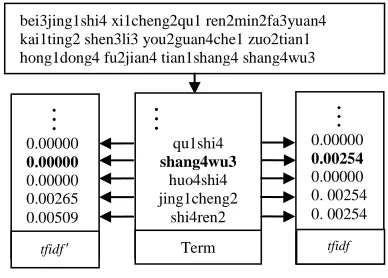
[image:3.612.92.289.122.396.2]in spoken document d .
Figure. 4. Vector Of Spoken Document For Tfidf (Right) And Modified Tfidf (Left)
Figure. 4 presents the difference of tfidf and modified tfidf. The top rectangle is the word list of a spoken document extracted from confusion network. The number in it is the tone of corresponding syllable. For tfidf, it tends to have the same weight because of the number of most word happening in the document only once. But for modified tfidf, the corresponding weight depends on the posterior probability, which may be different from the word happening only once. For the bold line, it shows that for some words with low posterior probability, the modified weight may be zero while the traditional tfidf weight will consider it as much important as others.
3. LOCALITY SENSITIVE HASH
Since normally the feature space is huge, like in our task, the dimension of vector space may be over ten thousands, it suffers from either space or query time that is exponential in the dimension. Locality sensitive hash is a new way to handle the problem of ‘the curse of dimensionality ’.
3.1 Basic Idea Of LSH
The key idea of locality sensitive hash is to hash the points in high dimensions using several hash functions to ensure that for each function the probability of collision is much higher for objects that are close to each other than for those that are far apart. Then, one can determine near neighbors by hashing the query point and retrieving elements stored in buckets containing that point.
For the point vin original spaceS ,B(v,r) represents the ball that the distance between the points in it and v are smaller than r, that is
} ) , ( | { ) ,
(vr q X d vq r
B = ∈ ≤ (3) whered(v,q)can be the distance in 1-norm or 2 norm space. If there is a family of hash function as H={h:S→U}, and in the space U after mapping it satisfies the following conditions, then this family of hash function is sensitive to locality.
C1: if q∈B(v,r1) , then PrH[h(q)=h(v)]≥p1
C2: if q∉B(v,r2), then PrH[h(q)=h(v)]≤ p2
wherer1<r2and p1> p2. These two conditions (C1 and C2) mean that if the point q is a neighbor of pointv, then after hash mapping, it will collide at a high probability, and vice versa. For a single hash function, it can map the point
vin high dimension space into a 1-dimension space like (4).
⋅ + =
l b v a v
ha,b( )
(4) Divided the 1-dimension space into segments, if each segment is treated as a bucket, can indicate which bucket the point is fallen in. Furthermore, the vector obeys the p-stable distribution to assure satisfies condition 1 and condition 2.
3.2 Indexing Based On LSH
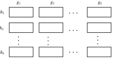
Single hash function can obtain only one value of each point after mapping, which is not enough to index the points of complicated situation in high space. In LSH approach, normally a family of hash functions is chosen to represent the location of the point in original space as in (5).
g(v)={h1(v),h2(v),...,hk(v)} (5) Thus by (5),
k
hash values can be obtained for the same point v, and each hash function hi(v) is a member of the hash family H . Usingk
hash values to represent the point v means the bei3jing1shi4 xi1cheng2qu1 ren2min2fa3yuan4kai1ting2 shen3li3 you2guan4che1 zuo2tian1 hong1dong4 fu2jian4 tian1shang4 shang4wu3
qu1shi4 shang4wu3huo4shi4 jing1cheng2
shi4ren2
Term
0.00000 0.00000 0.00000 0.00265 0.00509
0.00000 0.00254 0.00000 0. 00254 0. 00254
f
[image:3.612.94.288.261.400.2]mapping space is a k-dimension k
U instead of 1-dimension. Then in the space k
U it could provide more details to distinguish similar points. In common, this mapping procedure is done L times. We choose L functions as g1,g2,...,gL
from { : k}
U S g
G= → independently and
uniformly at random.
Based on the idea above, the indexing procedure is as follows:
Step 1: For training data, using VSM based on tfidf or modified tfidf to convert them into the points in high dimension space.
Step 2: Selecting proper ha,b(v) . We independently choose a valuing from 1-stable and 2-stable distribu-tions, and b is a real number chosen uniformly from [0,l].
Step 3: Selecting proper k and L, for each point v (training document), storing it in gj(v).
3.3 Parameters Selection In LSH
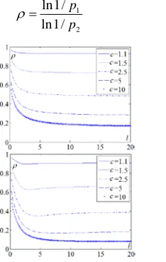
Except the parameters as a and b in (4), there are still many parameters should be chosen before indexing. In the condition 1 and condition 2, we hope the distance between p1 and p2 bigger. If we use ρ as follow, then we choose to keep ρ
small value.
2 1 / 1 ln
/ 1 ln
p p
=
ρ (6)
[image:4.612.304.522.70.249.2]
Figure. 5. The Relations Between L And ρ Under L1
Norm (Left) And L2 Norm (Right)
[image:4.612.143.260.451.636.2]
Figure. 6. The Relations Between C And ρ Under L1
Norm (Left) And L2 Norm (Right)
The relations between l, c and ρ are shown in Figure. 5 and Figure. 6 with c=r2/r1. It can be seen that l=4 is a better choice to assure the small ρ . Additionally, these four figures can reflect the effect of different c, which means the choice of l also depends on different datasets.
For the parameters k and L , they play important roles in accuracy and complexity of this approach. Normally the selection of these two parameters depends on the dataset. If for pointv , the probability of its neighbor point
qcan be found is 1−δ, then the follow equation represent the relation between k and L:
δ
− ≥ −
−(1 ) 1
1 1
L k
p (7) And Lcan be obtain according to (8).
− =
) 1 log(
log
1 k
p
L δ (8)
We select kaccording to the rule assuring the average time cost is minimized during following experiments.
3.4 Fast LSH
Supposing for each hash function ha,b(v), its time cost is O(d), the whole time consuming for each point is about O(dkL). Fast LSH aims to shorten the time consuming at the cost of independency of gj(v).
Let k be a even number, then we divide hash family into two parts {u1,u2}, where
u
1 andu
2are
)} ( ),..., ( ), (
{h1 v h2 v hk/2 v ,
)} ( ),..., ( ), (
[image:4.612.313.501.459.522.2]ISSN: 1992-8645 www.jatit.org E-ISSN: 1817-3195
set of hash functions as u={u1,u2,...us}, and randomly select two of them to generate gj(v). For the set u with s elements, there are
2 / ) 1 ( −
=s s
L different selections. Accordingly, the time consuming for each point is about
) (dks
O , which is much less than O(dkL). The weakness of this fast LSH lies in that there are only s independent hash families instead of L. 3.5 Classification Based On LSH
[image:5.612.296.511.230.338.2]LSH is mostly applied as indexing approach, and used for retrieval task. For classification task, after indexing on LSH, not only the training data are assigned into different buckets as Figure. 7, the labels of each training data are also stored in this hash structure.
Figure. 7. Hash Structure Built In Training Stage For a new point q (unknown document), we use the same set of hash functions as those in training stage to map this point into the buckets in Figure. 5. 2 points which firstly collide with L q
are used in classification. Two methods are presented to judge the class label of the new point. One is to select the nearest point with q among the 2 points, and regard these two points with L
the same label (1-nearest). The other one is to choose N nearest points, and assign the class label with most points to the point q (N-nearest).
4. EXPERIMENTS
In this section we present a set of experimental evaluations of our scheme based on LSH. We focus on 2-norm case, since this occurs most frequently in practice. The performance is evaluated by precision (P) and recall (R) rate.
4.1 Improvement Of Parameter l
From Figure. 5 and 6, it can be seen that for most applications, l should be selected as 4. But the selection of l also depends on different dataset. In this experiment, we adjust this value by the following algorithm.
Figure. 8 Selection Of L By Experiments Table 1 Classification Performance (%) For The Four Classes, National Defense (ND), Sports (SP), Country
Reports (CR) And Politics (PL) With Different l
ND SP CR PL mean
s
l=4 P 63.3 100. 0
72.2 77.8 78.3
R 96.7 6.7 96.7 93.3 73.4
l=1.4 1
P 69.8 100. 0
90.9 71.4 83.0
R 100.
0
6.7 100. 0
100. 0
76.7
In table 1, the weight is tfidf, and the classification approach is 1-nearest. Additionally,
hm equals to 11.2805 and num is 16. It can be seen that when l equals to 1.41, the system performance is better than those with l=4. In the following experiments, l is selected as 1.41. Furthermore from table 1, under both conditions for sports class, the recall rate is only 6.7%, which means most of sports documents are classified into other classes, such as national defense and country reports. It is also the reason why the precisions of those classes are low. The low recall rate of sports documents may lie in that there are many words intersection between sports and other classes. Moreover, tfidf does not care about the posterior probability. A word with low posterior probability plays the same role as those with high one. This will worsen the performance with words intersection.
4.2 Comparison Between Tfidf And Modified Tfidf
In this experiment, tfidf and modified tfidf weight are compared with 1-nearest classification scheme.
In table 2, from the average performance it can be found that the whole performance of modified tfidf is better than that of tfidf (l=1.41 in table 1). The main reason is the recall rate of sports, which has about 50% improvement. This result is caused by the proper counting of the tf part on posterior probability. In other experiments, modified tfidf is adopted.
1. Selecting a set of data randomly.
2. Computing the maximum of the hash value
hm by selecting hash function.
3. Dividing [-hm,hm] evenly into numparts and determining the num by experiments results, l=2hm/num.
...
...
...
...
...
...
g1 g2 gL
h1
h2
[image:5.612.98.287.298.396.2]Table 2 Classification Performance (%) For The Four Classes, National Defense (ND), Sports (SP), Country Reports (CR) And Politics (PL) With Modified Tfidf
ND SP CR PL means
tfidf ’ P 83.3 100.0 85.3 90.9 89.9 R 100.0 56.7 96.7 100.0 88.4
4.3 Comparison Between LSH And KD-Tree Table 3 presents the comparison of LSH and KD-tree classifier and 1-nearest and 7-nearest classification approaches. KD-tree is the most popular data structures used for searching in multidimensional spaces. The execution times of KD-tree and LSH are about 179.17ms and 39.62ms respectively.
Table 3 Classification Performance (%) For The Four Classes, National Defense (ND), Sports (SP), Country Reports (CR) And Politics (PL) With KD-Tree And LSH Classifiers
ND SP CR PL means
LSH P 83.3 100.0 85.3 90.9 89.9
1-nearest
R 100.0 56.7 96.7 100.0 88.4
KD-tree
P 88.2 100.0 88.2 85.7 90.5
1-nearest
R 100.0 56.7 100.0 100.0 89.2
LSH P 69.0 100.0 92.6 83.3 87.5
7-nearest
R 96.7 50.0 88.3 100.0 83.8
KD-tree
P 78.9 100.0 93.8 85.7 89.6
7-nearest
R 100.0 50.0 100.0 100.0 87.5
Although from average precision and recall rate, results of KD-tree are a little better than those of LSH, no matter for 1-nearest or for 7-nearest approaches, the consuming time of KD-tree is about 4.5 times of that of LSH. As for 1-nearest and 7-1-nearest approaches, it can be seen that the former one is better than the later one. The words overlap among different class can be viewed as noise, which makes the locations of points after mapping sensitive to the hash values. This can explain why the results of 7-nearest approach are worse than those of 1-nearest one.
4.4 Comparison between LSH and fast LSH
Table 4 Classification Performance (%) LSH And Fast LSH With 1-Nearest With National Defense (ND), Sports (SP), Country Reports (CR) And Politics (PL)
Since fast LSH selects only s independent hash families to spare the time consuming, there is a little reduction (less than 0.1%) both for precision and recall rate in table 4 compared with the LSH 1-nearest in table 3, while achieving about 46.7% execution time saving.
5. CONCLUSIONS
In this paper we present a new spoken document classification system on LSH. Confusion network is adopted to avoid the complicated word extraction on lattice, and posterior probability is considered to build the high dimensional space model. For LSH classification, the performance is compared with KD-tree. From the results of experiments, several conclusions can be drawn. Firstly, tfidf on posterior probability is better than traditional tfidf on the consideration of different effects on classification of words with high and low probability. Secondly, compared with KD-tree, LSH can spare about 4.5 times computing consuming with keeping the similar precision and recall rate. Thirdly, for 1-nearest and N-nearest classification methods, 1-nearest works better than N-nearest method under noisy condition (the large intersection words among different classes). At last, in real time applications, fast LSH can spare further time consuming with a little precision and recall rate lost.
6. ACKNOWLEDGMENTS
This work is supported by Young Teacher Support Plan by Heilongjiang Province and Harbin Engineering University in China (No.1155G17), and Fundamental Research Funds for the Central Universities in China.
REFERENCES
[1] P.D.Turney, P. Pantel, and others. From frequency to meaning: Vector space models of semantics. Journal of Artificial Intelligence Research, 37(1), 141-188 (2010).
Time(ms) ND SP CR PL means
ISSN: 1992-8645 www.jatit.org E-ISSN: 1817-3195
[2] S.M. Siniscalchi, C.H. Lee. A study on integrating acoustic-phonetic information into lattice rescoring for automatic speech recognition. Speech Communication, 51(11), 1139-1153(2009).
[3] Ariya Rastrow, Markus Dreyer, Abhinav Sethy. Hill climbing on speech lattices: a new rescoring framework. ICASSP 2011, 5032-5035.(2011)
[4] G.Cosma, M. Joy. An approach to source-code plagiarism detection and investigation using latent semantic analysis. IEEE Transactions on Computer, 61(3), 379-394(2012).
[5] IT Jolliffe. Principal Component Analysis. New York: Springer Verlag. (2002).
[6] A. Andoni, Indyk P. Near-optimal Hashing algorithm for approximate nearest neighbor in high dimensions. Communications of ACM. 51(1), 117-122 (2008).
[7] Huang Yongming; Zhang Guobao; Li Xiong; et al. Improved Emotion Recognition with Novel Global Utterance-level Features. applied mathematics & information sciences. 5 (2): Special Issue: 147-153 (2011).
[8] Z Lei, C Guoxing, X Xuezhi, C Jingxin. Topic Mining based on Word Posterior Probability in Spoken Document. Journal of Software. 6(11): 2292-2299 (2011)
![Assessment of Physiological Health Status in Relations to Different Anthropometric and Cardio respiratory Measures of Head Supported Load Carrying Male Porters of Sikkim, India [Article Retracted]](data:image/gif;base64,R0lGODlhAQABAIAAAP///wAAACH5BAEAAAAALAAAAAABAAEAAAICRAEAOw==)