Agent Based Modeling in Supply Chain Management:A Genetic Algorithm and Fuzzy Logic Approach

Agent-Based Modeling in Supply Chain

Management:A Genetic Algorithm and

Fuzzy Logic Approach

Djennas, Meriem and Benbouziane, Mohamed and Djennas,

Mustapha

Université d’Amiens, France, faculté des sciences économiques et de

gestion Tlemcen, University of Tlemcen, faculté des sciences

économiques et de gestion Tlemcen, University of Tlemcen

September 2012

Online at

https://mpra.ub.uni-muenchen.de/87438/

DOI : 10.5121/ijaia.2012.3502 13

A

GENT

-

BASED

M

ODELING

I

N

S

UPPLY

C

HAIN

M

ANAGEMENT

:

A G

ENETIC

A

LGORITHM AND

F

UZZY

L

OGIC

APPROACH

1

Meriem DJENNAS,

Mohamed BENBOUZIANE and

Mustapha DJENNAS

1

Department of Economics, Amiens University, Amiens, France

meriemdjennas@gmail.com

2

Department of Economics, TlemcenUniversity, Tlemcen, Algeria

mbenbouziane@yahoo.fr

3

Department of Economics, TlemcenUniversity, Tlemcen, Algeria

djennasm@yahoo.fr

A

In today’s global market, reaching a competitive advantage by integrating firms in a supply chain management strategy becomes a key success for any firm seeking to survive in a complex environment. However, as interactions among agents in the supply chain management (SCM) remain unpredictable, simulation appears as a powerful tool aiming to predict market behavior and agents’performance levels. This paper discusses the issues of supply chain management and the requirements for supply chain simulation modeling. It reviews the relationships amongArtificial Intelligence (AI) and SCM and concludes that under some conditions, SCM models exhibit some inadequacies that may be enriched by the use of AI tools. This approach aims to test the supply chain activities of nine companies in the crude oil market. The objective is to tackle the issues under which agents can coexist in a competitive environment. Furthermore, we will specify the supply chain management trading interaction amongagents by using an optimization approach based on a Genetic Algorithm (AG), Clustering and Fuzzy Logic (FL).Results support the view that the structured model provides a good tool for modeling the supply chain activities using AI methodology.

K

Supply Chain Management, Genetic Algorithm, Fuzzy Logic, Clustering, Optimization.

1. I

14

When the environment reaches a high level of complexity, agents with limited cognitive capacities can’t behave rationally; they adopt a simple decision procedure to reach a satisfying level of results for different situations. When acting in a given environment, the agent learns from a training process by trading off other procedures with the used one. They become hypotheses about the environmentto be tested. If the agent considers that one of these hypotheses could provide a better result if it was effectively used, it would become the main one. Consequently, the new rules are produced by a process of weighting the best old ones. This kind of learning is typically an evolutionary learning. The mechanism that allows showinghow to learn and interact in the environment as well as to develop strong decision procedures is called a Genetic Algorithm (GA), (Holland, 1975).

Moreover, since some market systems are highly complex and can’t be easily modeled only by one AI tool, there is actually a growing tendency to gain more visibility by integrating the fuzzy logic approach in combination with neuro-computing and genetic algorithms. In this paper, a hybrid methodology is developed by combining Genetic Algorithm (GA), Clustering and Fuzzy

Logic (FL) approaches for a precise and effective evaluation of agents’ performance in a SCM. It

keeps a set of fuzzy rules with their membership functions and uses the results of GA to determine the importance of the decision rules in a SCM. The proposed fuzzy system is used to generate the performance percentage of the agent through the adoption of fuzzy inference system (FIS) in the MATLAB fuzzy logic toolbox platform. Furthermore, the optimization of the artificial market model integrates the interaction amongautonomous decision-makers. Then, simulations are conducted tooptimize market’s conditions (first step) and to analyze all decisions linked to the internal cognitive structure of the agents (second step). This helps autonomous decision-makers to improve their decision performance through adaptation and training processes within a Supply Chain Management.

2. S

C

M

(SCM)

The supply chain Management (SCM) concept can be defined as a series of activities, processes and organizations that help to move materials (both tangible and intangible) from initial suppliers to final customers (Waters, 2007). Due to its considerable competitive impact, the concept relates systemically to the integration of organizational functions ranging from the ordering and receipt of raw materials through the manufacturing processes to the distribution and delivery of products to end users with a view to enabling organizations to achieve higher quality products and greater customer services(Stevens, 1989).

2.1. Supply chain modeling

2.1.1 Brief literature review

15

simulation. Lee and Kim (2002) developed a hybrid approach that combines analytic and simulation models.Joineset al. (2002) studied a supply chain simulation optimization methodology employing GA to optimize system parameters, using sa hybrid algorithm that combines mathematical programming and a simulation model of a manufacturing system for the multi-period and multiproduct production planning problem (Byrn and Bakir, 1999; Kim, 2001).

2.1.2. Supply chain performance measures

In general, performance measures can be classified as either qualitative orquantitativein nature (Felix and Chan, 2004). In the qualitative performance measures there is no direct numerical measurement, although some aspects may be quantified like customer satisfaction, flexibility, information and material flow integration, effective risk management, supplier performance, etc. Quantitative performance measures can be described numerically. Quantitative supply chain performance measures may be categorized by objectives based on cost or profit (cost and inventory minimization, sales, profit maximization,return on investment, etc.) and, measures of

customer responsiveness (occupancy rate maximization, product delay minimization, lead time

minimization, etc.), andproductivity(capacity maximization, resources maximization, etc.).

The modeling approach used in this paper can be classified into the first category. Anderson et al. (1989) stated that in measuring logistics performance, a comprehensive strategy of measurement is necessary for the successful planning, implementation and control of the different activities comprising the business logistics function. Stainer (1997) advocated that a set of performance measures is needed in order to determine the efficiency and/or the effectiveness of an existing system, or to compare competing alternative systems.

2.1.3. Supply chain management model

According to Ingalls(1998), two techniques can be employed for the SCM performance evaluation, namely, mathematical optimization and simulation. In this paper, a crude oil market has been chosen as simulation case1. Because of the existence of a huge number of agents and the importance of the oil market volume, it appears that it would certainly be difficult to get a perfect modeling process; nevertheless, the most important operating ones are introduced. For example, the export volume has been selected for supplier agents. On the other hand, intermediate and industrial agents (American Multinationals so-calledsuper majorsin the oil industry) have been selected on the basis of financial criteria. We have chosen nine artificial agents2 (fictitious and real agents) that contribute efficiently within inter-organizational activities (transactions, information exchange, horizontal integration and upstream/downstream integration). The artificial market architecture can be represented as follows:

1

The reader can refer to EIA website (Energy Information Administration www.eia.doe.gov), a governmental organization that diffuse a considerable and various volume of information about the worldwide energy market by country, companies, etc.

16 2.1.3.1. Market actions hypotheses

Every agent iacts on the market at the instant t with a certain wealth Wi and a performance

Feat(t). Agent’s wealth is made up by its cash money CMi and its reserves of stock of products

S(t). At period t, the Qpro, Qint, Qind quantities of product respectively from producers, intermediates and industrials are sold or bought at the market equilibrium price PE. Every agent must choose a quantity of product Qi at every period t by considering a set of constraints, for example the stockS. Its objective is to maximize its wealth at each period of transition. Supplier and industrial agents receive demand orofferbids from intermediate agent as a purchase or sale act. In addition, the following hypotheses are assumed (Mathieu etal., 2006):

- Hypothesis 1: the exchange occurs exclusively just after the determination of the market

equilibrium pricePEfor period t.

- Hypothesis 2: every agent tries to maximize its performance function based on the

strength of his prediction as well as his wealth through the learning experiences.

- Hypothesis 3: as agent predictions are based upon past experiences, they are not perfectly

rational. So market equilibrium is determined by interactionsamongthem.

- Hypothesis 4: the equilibrium pricePEis communicated to agents as the start off price in

periodt+1.

- Hypothesis 5: the market price P is endogenous; it is determined by interactions

amongagents possessing in different levels of perception.

- Hypothesis 6: there are no horizontal interactions amongagents except the information exchange.

2.1.3.2. Criteria and rules of decision

- Rule 1: every supplier agent adopts an action at the instant tas a pair-decision (Q,SP), whereQis the product quantity offered andSPthe transaction selling pricePrecorded at the end oft-1.

- Rule 2: every intermediate agent adopts an action at the instanttas a triplet-decision(Q,

PP, SP), where Q is the product quantity, PP and SP are respectively purchasing and

selling prices.

Figure1. Supply chain model

Macro Environment

Level 1

Level 2

Level 3

T

ra

n

sa

ct

io

n

al

p

ro

ce

ss

d

ir

ec

ti

o

n

Transactional flow Informational flow

Informational micro environment

L1/Agent 1 L1/Agent 2 L1/Agent 3

L2/Agent 3 L2/Agent 2

L2/Agent 1

L3/Agent 3 L3/Agent

17

- Rule 3: every industrial agent adopts an action at the instant tas a pair-decision(Q,PP),

whereQis the product quantity to buy andPPthe purchasing price.

- Rule 4: returnr(t)of an action at the period tis defined by the agent wealthWvariation

amongt-1andt.r(t) = W(t) - W(t-1).

- Rule 5: the agent stated evaluation EX(t) at the instant tis calculated by the sum of its return and its Price Precision DegreePPD.E(X(t)) = r(t)+[-|PPD(t)|].

- Rule 6: The agent performanceFeat(t)at the instant tis the accumulated sum of it past

evaluations till the periodt.Feat(t)=∑ [E(X(t))].

- Rule 7:PPDis the difference amongthe absolute values of the expectedvariation E(Δ P)

andrealvariationR(Δ P)of prices. It is calculated as follows:PPD=|E(Δ P)| - |R(Δ P)|. - It is noted that as the agent acquires experience, he gains then the ability to develop his

business memory and value the results accumulated over time through an exchange process.

2.2. Exchange process

Industrial agents coming from the third level of the SC, get into the market with a double anticipation as far as demand and purchasing price are concerned. They communicate their prices and quantities to intermediate agents (SC second level). Logically, prices proposed by industrials are lower than those proposed by intermediates. The market game starts with price adjustments where every industrial agent tries to increase steadily his price, and at the same time each intermediate agent tends to decrease gradually his price. The game is over at an equilibrium price determined through a consensus. As for quantities, the industrial agent who sets up the highest purchasing price becomes the first one who ends up his transaction (purchasing the needed quantity) with the intermediate agent that proposes the lowest selling price. The industrial agent that proposes the second superior purchasing price is the second one who achieves his transaction thereafter with the intermediate actor who proposes the second lower selling price and so forth. This means that the industrial agent that proposes the lowest purchasing price incurs the risk of not satisfying his demand (purchasing a lower quantity than his needs). Moreover, the intermediate agent who proposes the highest selling price incurs the risk of not materializing his offer (selling a lower quantity).The price’s game remains the sameamongthe SC first level agents and those of the second level. So, the intermediate agents who were sellers become purchasers in this case. Quantification of this process will be optimized through a simulation based on a Genetic Algorithm.

3. G

A

The GA, considered nowadays as one of the most used simulation tools, is applied in the resolution of several types of linear and non-linear optimization problems (Goldberg, 1989; Davis, 1991). However, in real problem conception of supply chains decisions, we encounter multiple choices as far as inter-organizational relationships are concerned. Here, the existence of couples of different performance levels hypothesis and inter-organizational situations is preferred. Consequently, the optimization parameters are defined as follows:

Fitness function: performance Feat(t): the agent’s performance is the sum of his accumulated

18

1

( ) ( )

1 t

t t cumulated

t

feat

E X

feat

−

=





=

_

_

+

∑

Adjustment variables: are the price P and quantity Q that help an agent to reach the highest value of the fitness function.

Constraint variables: although there are several conditions of positivity in the supply chain model, the GA defines only one constraint variable to be verified for all artificial agents, i-e the wealth W that must be positive without exceeding the determined bounds. In addition to this common constraint, we add some other specific constraints for every level: the unit extraction cost of a crude oil barrel must not be lower than a threshold valueC0for all producer agents. The

unit margin for level 2 and 3 agents must not be lower to the threshold values: UM0. Before

choosing the parameters and presenting some results, we shall present the GA model architecture.

3.1. Model optimization architecture

The objective is to preserve the supply chain architecture where for each agent a performance function is maximized under constraints of costs and profit: (i)Max: Feat(x), (ii)under

constraints:W(x)≥ 0, C(x) ≥ C0(SC first level agents), MU(x)≥ MU0(SC second and third level

agents), and clearing market conditions (agents cannot randomly consume all stocks as they want. For each buyer there is a seller and vice-versa).

It should be considered that better results can be obtained if bounds are not integrated in the GA simulations. In this case, the GA can push up quantity volumes or price values or even reduce

costs in order to increase the agent’s wealth and performance, whereas if bounds are taken into

consideration, and under the assumption of market rationality, each agent can’tincrease prices or quantities as much as he likes since these variables are defined in term of competition and interactions amongagents. Our simulations have been run with MATLAB. The GA parameters were defined after ten simulations. Each combination of the different types of parameters gave a performance level. It is noted that the choice of the parameters is mainly based on the nature of the problem3.

3.2. Genetic algorithm parameters

The fitness function is specified by the type of the population under study. For simplification reasons, we have chosen a double vector fitness function where creation, crossover and mutation functions are generated by the algorithm itself. The parameters are: population size 100 individuals; uniform creation function; uniform stochastic selection; reproduction function based on an elite strategy; Gaussian mutation function; scattered crossover function and tolerance function: 1e-30.

During the first simulation tests, a generation of 500 individuals was considered. However, the GA did not reach a steady threshold so that more improvement of the fitness function could not be achieved. In a second stage, a generation of 1000 individuals was considered. Results were more satisfactory for some agents but not for others. Since, on the basis of the number of parameters and the information flows introduced in the optimization model, the plot of the fitness function began to stabilize around a threshold only after the 1000thgeneration for certain agents, namely the intermediate ones. Therefore, a generation of 1500 individuals was considered in

3

19

0 5 10 15 20 25

0 0.5 1 1.5 2 2.5 3 3.5 4 4.5

5x 10 7

Tim e periods

W e a lt h W ( 1 0

3 M

D )/ F e a t (N M )

SC level 2 W ealth and Feat evolution

N-OPW N-OPF OPW OPF

0 5 10 15 20 25

0 2 4 6 8 10 12 14 16x 10

7

Tim e periods

W e a lt h W ( 1 0

3 M

D )/ F e a t (N M )

SC level 1 W ealth and Feat evolution

N-OPW N-OPF OPW OPF

order to ensure the GA convergence for all agents. The used learning database contains 27 data points, each one representing one period of time.

3.3. Genetic Algorithm optimization results

3.3.1. Supply chain results for first level agents

20

0 5 10 15 20 25

0 0.5 1 1.5 2 2.5 3 3.5 4 4.5

5x 10

7

Time periods

W

e

a

lt

h

W

(

1

0

3 M

D

)/

F

e

a

t

(N

M

)

SC level 3 W ealth and Feat evolution

N-OPW N-OPF OPW OPF

3.3.3. Supply chain results for third level agents

The simulation results show the performance Feat and wealth W graphs for the nine agents. Obviously, with the GA, agents have reached higher performance and wealth levels under the same market conditions as in the case of non-optimized market data. However, until nowwe don’t

know the contribution of the decision variables (price P and quantity Q) within the agent’s

performance function. By introducing a Fuzzy Logic (FL) analysis, we can explain the internal cognitive structure of agents and achievea clearerresult as far as agents’ performancemodeling is concerned.

4. M

’

In this section we’ll attempt to understand the relationship among the generated agents’

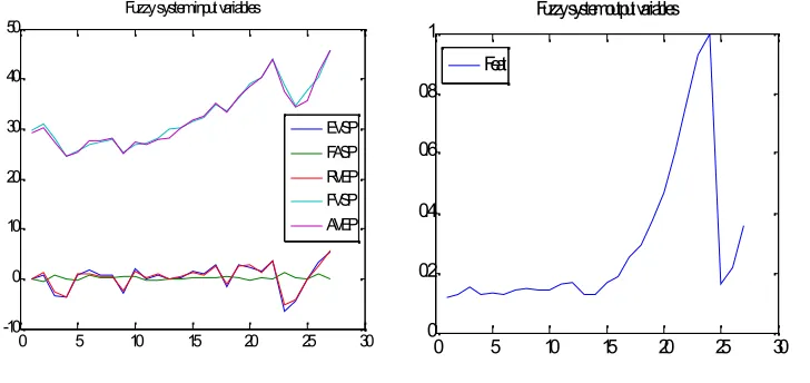
performance from the intrinsic and the extrinsic decision factors. Two cases are considered: market with non-optimized data and market with GA-optimized data. Each case considers the following factors (table 1): expected variation of selling price (EVSP), forecast accuracy of selling price (FASP), real variation of buying/selling equilibrium market price (RVEP), actual value of selling equilibrium price (AVEP) and forecasted value of buying/selling price (FVPP/FVSP) by consideringonlyprices information, and agent relative quantity demand/supply (ARQS) when considering pricesandquantities information. In the model, we integer one output

variable: agent’s performance (Feat).

In the two cases, the decision information structure is tested in relation with two decision variables: prices and quantities. The objective is to understand the importance of the two sets of information within an agent decision process. Therefore, the differences in the input data sets are shown in the fifth row of the input data (table 1). First, we consider information on price and,

21

0 5 10 15 20 25 30

-10 0 10 20 30 40 50

Fuzzy system input variables

EVSP FASP RVEP FVSP AVEP

0 5 10 15 20 25 30

0 0.2 0.4 0.6 0.8 1

Fuzzy system output variables

Feat

the agent in the total market supply: ARQS = AQS/MS (where AQS is the agent’s supply

quantity and MS the market supply).

Table 1.Influence and decision variables in an agent model

* SC first level: FVSP. Second level: FVPPandFVSP. Third level: FVPP

Consequently, these factors will be addressed as inputs and the generated agent performance will be presented as output. Therefore our problem tackles five input variables and one output variable for the first and third levels of the supply chain agents, and six input variables and one output variable for the second level. The number of rows in input and output sets is 27 representing, the number of examples or samples or data points available. For example, a row in the input set of an agent from the first level represents a set of values for the five input variables (EVSP, FASP, RVEP, AVEP and FVSP or ARQS); and the corresponding row in the output set represents the observed value for the agent performance (Feat).

The relationship among the input variables and the output variable is modeled by the first clustering data. The cluster centers will then be used as a basis to define a Fuzzy Inference System (FIS) which can be used to explore and understand agent performance level. We’ll present the implemented methodology for only one agent from the artificial market (the first

agent in the first level of SC). For the rest, we’ll show only the results of the Fuzzy Interference

System (FIS).The following two graphs show the input and output data concerning the first agent

22

5. C

F

L

While clustering allows grouping input data into broad precise categories allowing an easier understandability, fuzzy logic is an effective paradigm to handle imprecision. It can be used to take fuzzy or imprecise observations for inputs and yet arrive at precise values for outputs (Bezdek, 1981). Also, the Fuzzy Inference System (FIS) is a simple way to build some systems without using complex analytical equations (Chiu, 1994). In our case, fuzzy logic will be employed to capture the broad categories, identified during clustering, into a Fuzzy Inference System (FIS). The FIS will then act as a model that reflects the relationship among input decision factors for each agent and its performance. Therefore, both clustering and fuzzy logic provide a simple but powerful way to model the supply chain in order to understand the contribution of crucial factors that influence the agent performance in both market cases: optimized and non-optimized. Before presenting the clustering-FIS relationship and FIS data exploration, Clustering and Fuzzy Logic concepts are briefly discussed.

5.1. Clustering

5.1.1. Overview

A number of techniques can be used to solve clustering problems including matrix formulation, graph theory and artificial intelligence (AI) (Serber, 1984). A comprehensive representation and a hierarchical model of a supply chain are fundamental for the incorporation of the multiple decision-making levels and optimization process (Khoo and Yin, 2003). Typically, in optimizing a supply chain, customer orders, product flows, supply chain units, transportation, customer service level, other resources and constraints, are used as inputs in a simulation or an optimization program so as to derive a product plan.

As already mentioned, a complex supply chain optimization problem can hardly be solved only by the use of an AI tool. An approach based on clustering is proposed here to reduce the search space. The approach is likely to help to set efficiently the near optimal or at least some good-enough solutions for a complex supply chain (Khoo et al., 2000).

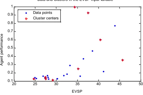
5.1.2. Clustering the market data

First, a clustering technique called subtractive clustering is used. Subtractive clustering (Chiu, 1994) is a fast one-pass algorithm for estimating the number of clusters and the cluster centers in a dataset. Consequently, data to be clustered are introduced in order to mark a cluster’s radius of

23

20 25 30 35 40 45 50

0.1 0.2 0.3 0.4 0.5 0.6 0.7 0.8 0.9 1

EVSP

A

g

e

n

t

p

e

rf

o

rm

a

n

c

e

Data and Clusters in the EVSP input variable

Data points Cluster centers

Table 2.Data subtractive clustering for the first agent in the SC first level

The Clusters matrixChas nine rows representing nine clusters with six columns representing the positions of the clusters in each dimension. For example, the following plot shows how the clusters have been identified in theEVSPandFeatdimensions of the input space. The variableS contains thesigmavalues that specify the range of influence of a cluster center in each of the data dimensions. All cluster centers share the same set ofsigmavalues.Shas six columns representing the influence of the cluster centers on each of the six dimensions.

5.2. Fuzzy Logic

24

0 2 4 6 8 10

0 0.2 0.4 0.6 0.8 1

Figure. Gaussian membership function c

Sig

mechanism for doing this is a list of if-then statements called rules. All rules are evaluated in parallel, and the order of the rules is unimportant.

5.2.1. Fuzzy Inference System (FIS)

After using fuzzy clustering, the second step is to create a FIS on the basis of subtractive clustering taken from the cluster centers and their range of influences. The first argument in a FIS is the input variables matrix and the second argument is the output variables matrix represented by membership functions and the fuzzy inference type.

5.2.2. Membership Functions

A membership function (MF) is a curve that defines how each point in the input space is mapped to a membership value (or degree of membership) among 0 and 1. The function itself can be an arbitrary curve that may be defined on the basis of simplicity, convenience, speed, and efficiency. A fuzzy set is an extension of a classical set. If X is the universe of discourse and its elements are denoted by x, then a fuzzy setAinXis defined as a set of ordered pairs.

A = {x, µA(x) | x∈X}. [2]

µA(x) is called the membership function (or MF) of x in A.

There are many types of membership functions. The simplest types are formed using straight lines. Of these, the simplest is the triangular membership function. These straight line membership functions have the advantage of simplicity. The use of Sugeno-type inference system (see the next paragraph) transforms the membership functions into Gaussian ones. The symmetric Gaussian function depends on two parameters _{andcas given by:}

2 2

( )

2

( ; , )

x c

f x

_

c

e

− −

=

25 5.2.3. Fuzzy Inference type

Fuzzy inference is the process of formulating the mapping from a given input to an output using fuzzy logic. There are two types of fuzzy inference systems that can be implemented in the MATLAB Fuzzy Logic Toolbox: Mamdani-type and Sugeno-type. The two types of inference systems vary somewhat in the way outputs are determined. Mamdani-type inference developed in by EbrahimMamdani (Mamdani, 1975), assumes the output membership functions to be fuzzy sets. After the aggregation process, there is a fuzzy set for each output variable that needs defuzzification. Sugeno or Takagi-Sugeno-Kang method of fuzzy inference was introduced in 1985 (Sugeno, 1985), it is similar to the Mamdani method in many respects. The first two parts of the fuzzy inference process, i-e, fuzzifying the inputs and applying the fuzzy operator, are exactly the same. The main difference amongMamdani and Sugeno is that the Sugeno output membership functions are either linear or constant. A typical rule in a Sugeno fuzzy model has the form:

If Input 1 = x and Input 2 = y, then output is z = ax + by + c

For a zero-order Sugeno model, the output level z is a constant (a=b =0).The output levelziof

each rule is weighted by the firing strengthwiof the rule combining membership functions for the

considered inputs. The final output of the system is the weighted average of all outputs.

5.3. Clusters-FIS relationship

A FIS is composed of inputs, outputs and rules. Each input and output can take any number in the membership function. The rules dictate the behavior of the fuzzy system based on inputs, outputs and membership functions. The FIS attempt to capture the position and influence of each cluster in the input space.

Since our dataset has five (or six)input variables and one output variable, the FIS has five (or six) inputs and one output. Each input and output has as many membership functions as the number of identified clusters. As seen previously, nine clusters are identified for the first agent in the first SC level. Therefore, each input and output will be characterized by nine membership functions. Also, as the number of rules equals the number of clusters, nine rules are then created.

We can now probe the FIS to understand how the clusters get converted internally into membership functions and rules and we’ll try to analyze how the cluster centers and the

26

succinctly maps cluster1 in the input space to cluster1 in the output space. Similarly the other eight rules mapcluster2tocluster9in the input space tocluster2tocluster9in the output space.

If a data-point closer to the first cluster (or in other words having strong membership to the first cluster) is fed as input to the FIS, then the first rule will fire with more firing strength than the other rules. Similarly, an input with strong membership to the second cluster will fire the second rule with more firing strength than the other rules and so on. The output of the rules (firing strengths) is then used to generate the output of the FIS through the output membership functions. The one output of the FIS (Feat) has nine linear membership functions representing the nine clusters identified. The coefficients of the linear membership functions though are not taken directly from the cluster centers. Instead, they are estimated from the dataset using least squares estimation technique:

(

)

n

i i

i

Act Exp

MSE

N

=

−

=

∑

Where N is the number of fuzzy rules, Acti and Expi the actual and the expected output

respectively. All the nine membership functions will be a part of the following linear form:

a.[EVSP] +b.[ FASP] +c.[ RVEP] +d.[ FVSP] +e.[ AVEP] +f. [5]

Wherea,b,c,d,eandfrepresent the coefficients of the linear membership function.

By modifying the values in the membership functions, we can observe some changes in the parameters so that new performance percentage is attributed to the decision variables.

5.4. FIS graphical data exploration

27

The graph shows the output surface for two inputs EVSP and FASP. As we can see, and this may sound to be rational, as the Feat increases, FASP decreases. By simulating the FIS response for specific values of the input variables, we can understand how Feat will occur for a particular input setup; say a certain value of EVSP, FASP, RVEP, AVEP and FVSP and so on. This process helps simulate the FIS response for the input of our choice.

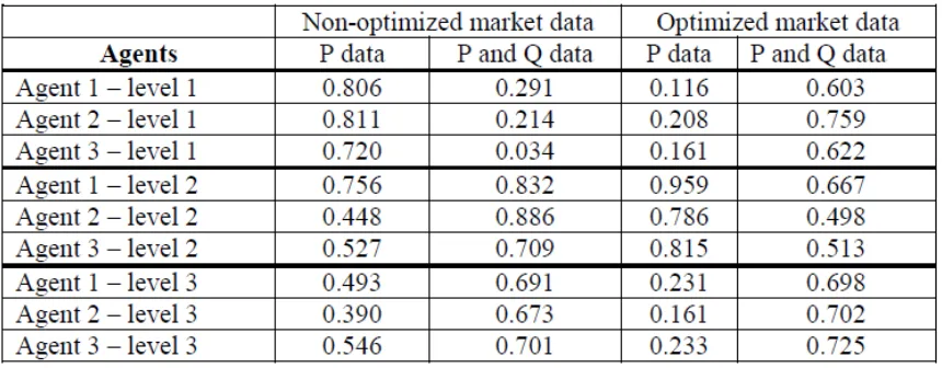
The next table shows the whole set of results upon considering the two markets cases as illustrated above. By exploring the table, we can understand the importance of the two decision variables, PandQ, in building the agent performance level. The table shows the contribution of decision variables in the agent performance process (learning process).

Table 3. Decision variables and their contribution in the agent performance level

6.G

The genetic algorithm optimization has allowed to set a re-attribution of the price/quantity mechanism for all agents so that each one succeeds in maximizing his wealth Wto acquire a rich enough knowledge basis needed to improve his prediction ability ofprices. Therefore, the accumulated fitness succeeds for each rule. At every period/test, each agent uses the rule that helps him to win the highest accumulated fitness. After a certain number of tests,the agent proceeds to change his hypotheses about the real worldfor adaptation purposes. This is reached through a mechanism where the new rules are produced from the best old rules via selection, crossover and mutation of the genetic algorithm operators.

28

have developed a selfish behavior that impacted the market conditions for a non-cooperative game expressed by lower agents’ performance levels in comparison with the optimized market case (see GA results’ graphs).

However, the situation in the second level seems different. Due to a co-managed inventory for both level 1 and level 3 agents, transactions of second level agents are quickly fulfilled. Although

cooperation exists also in this level, the average agent’s performance is mainly influenced by information about prices, and the addition of the information on quantity doesn’t appear to be

important within the agent performance and cognitive structure particularly when considering non-optimized market data (table 3). Furthermore, contrary to all expectations, the optimized market data show that the price information is more important in building agent performance (with 95.9%, 78.6% and 81.5% for the three agents respectively). The reason may be due to the fact that level 2 agents model is too complicated so that a decision takes a longer time because of the importance of the volume of information to be treated compared to other agents models.

On the other hand, as the resource utilization is more important for third level agents, information about quantities have a better utilization compared to agents in level 2. This can be expected since the third level agents make decisions undersupplier’s inventory levelconstraints. For example, if

the order exceeds the first supplier’s limit, the remaining quantity should be completed by the next supplier. That means agents will keep a certain level of inventory. In addition, the performance reached by optimized market data is better than the non-optimized ones, so that agents in level 3 should consider cooperation as far as the inventory management with their suppliers (agents in level 2) is concerned.

On the whole, we can say that non-cooperative market model seems to be less appropriate than the cooperative market model in terms of agents’ performance. Therefore, data without GA

optimization have not outperformed the inter-organizational supply chain model.

This experience suggests that advanced research developed through the genetic algorithm and fuzzy logic theories provides some very interesting instruments to build economic models concerned with decision theory that help to establish strong relationships among the system and the psychological aspects of agents.

7. C

In recent years, many research papers have focused on the performance measurement of a supply chain model that involved varieties of simulation software packages. In this paper, we have attempted to show how Genetic Algorithm, Clustering and Fuzzy Logic can be employed as effective techniques for data modeling and analysis in a supply chain management process. The principle was to evaluate cooperation and coordination among agents at different levels of interactions (upstream and downstream).

29

Further research can be carried out by increasing the number of parties involved in order to see what will be the effects of different levels in such complex system since the new competitive paradigm is based on the competition among different supply chains rather than the competition among a set of companies in a market. Nowadays, this new tendency confirms the fact that the success of any one company will depend fundamentally upon how well it manages its supply chain relationships.

8. R

[1] Anderson P., Aronson H., Storhagen N.G. (1989)‘‘Measuring logistics performance”. Engineering

Costs and Production Economics, vol. 17, p. 253–262.

[2] Androdottir S. (1998), Handbook of simulation. Wiley, New York, p. 307–334.

[3] Bezdek J.C., (1981), Pattern Recognition with Fuzzy Objective Function Algorithms, Plenum Press, New York.

[4] Byrn M.D., Bakir M.A., (1999),‘‘Production planning using a hybrid simulation-analytical approach”.

Journal of Production Economics, vol 59, p. 305–311.

[5] Chiu S. (1994), ‘‘Fuzzy Model Identification Based on Cluster Estimation”, Journal of Intelligent and

Fuzzy Systems, vol. 2, p. 3.

[6] Davis L. (1991), Handbook of Genetic Algorithm, Van Nostrand, Reinhold, New York. [7] Energy Information Administration www.eia.doe.gov

[8] Evans G.N, Naim M.M.&Towill D.R., (1998), ‘‘Application of a simulation methodology to the redesign of a logistical control system”, Journal of Production Economics, p. 56–57/157–168.

[9] Felix T.S., Chan H.K. (2004), Simulation modeling for comparative evaluation of supply chain management strategies. Springer-Verlag London Limited.

[10] Fu M., (2001), ‘‘Simulation optimization”, Proceedings of the 2001 Winter Simulation Conference, p.

53–61.

[11] Goldberg D.E., (1989), Genetic Algorithm in Search, Optimization and Machine Learning, Addison Wesley, Reading, MA.

[12] Holland J.H., (1975), ‘‘Adaptation in Natural and Artificial Systems”, The University of Michigan

Press.

[13] Ingalls R.G., (1998), ‘‘The value of simulation in modeling supply chain”. Proceedings of the 1998

Winter Simulation Conference, p. 1371–1375.

[14] Joines J.A., Kupta D., Gokce M.A., King R.E., Kay M.G., (2002), ‘‘Supply chain multi-objective

simulation optimization”. Proceedings of the 2002 Winter Simulation Conference, p. 1306–1314. [15] Khoo L.P., Lee S.G., Yin X.F., (2000), ‘‘A prototype genetic algorithm-enhanced multi-objective

dynamic scheduler for manufacturing systems”, International Journal of Advanced Manufacturing

Technology, vol. 16, p. 131-138.

[16] Khoo L.P., Yin X.F., (2003), ‘‘An extended graph-based virtual clustering-enhanced approach to

supply chain optimisation”, International Journal of Advanced Manufacturing Technology, vol. 22, p.

36-47.

[17] Kim B., Kim S. (2001), ‘‘Extended model of a hybrid production planning approach”. Journal of

Production Economics,vol. 73, p. 165–173.

[18] Lee Y.H, Cho M.K., Kim S.J., Kim Y.B., (2002), ‘‘Supply chain simulation with discrete-continuous

combined modeling”, Computer Industrial Engineering, vol 43, p. 375–392.

[19] Lee Y.H., Kim S.H., (2002), ‘‘Production-distribution planning in supply chain considering capacity

constraints”. Computer Industrial Engineering, vol. 43, p. 169–190.

[20] Mamdani E.H., Assilian S., (1975), ‘‘An experiment in linguistic synthesis with a fuzzy logic controller”, International Journal of Man-Machine Studies, vol. 7, p. 1-13.

[21] Mathieu P., Beaufils B., Brandouy O., (2006), Artificial Economics, agent-based methods in finance, game theory and their applications, Springer.

[22] Stainer A., (1997) ‘‘Logistics - a productivity and performance perspective”, Supply Chain

30 [23] Serber G.A.F., (1984), Multivariate Observations, Wiley.

[24] Stevens, G.C., (1989),‘‘Integrating the supply chain”, International Journal of Physical Distribution

and Materials Management, Vol. 19 No. 8, p. 3-8.

[25] Sugeno M., (1985), Industrial applications of fuzzy control, Elsevier Science Pub. Co.

[26] Waters D., (2007), Global logistics new directions in Supply Chain Management, MPG Books Ltd, Bodmin, Cornwall.