Munich Personal RePEc Archive
Two-agent Nash implementation: A new
result
Wu, Haoyang
5 April 2011
Online at
https://mpra.ub.uni-muenchen.de/30068/
Two-agent Nash implementation:
A new result
Haoyang Wu
∗
Abstract
[Moore and Repullo,Econometrica58(1990) 1083-1099] and [Dutta and Sen,Rev. Econom. Stud. 58(1991) 121-128] are two fundamental papers on two-agent Nash
implementation. Both of them are based on Maskin’s classic paper [Maskin, Rev. Econom. Stud.66(1999) 23-38]. A recent work [Wu, http://arxiv.org/abs/1002.4294, Inter. J. Quantum Information, 2010 (accepted)] shows that when an additional condition is satisfied, the Maskin’s theorem will no longer hold by using a quantum mechanism. Furthermore, this result holds in the macro world by using an algorith-mic mechanism. In this paper, we will investigate two-agent Nash implementation by virtue of the algorithmic mechanism. The main result is: The sufficient and nec-essary conditions for Nash implementation with two agents shall be amended, not only in the quantum world, but also in the macro world.
Key words: Quantum game theory; Mechanism design; Nash implementation.
1 Introduction
Game theory and mechanism design play important roles in economics. Game theory aims to investigate rational decision making in conflict situations,
whereas mechanism design just concerns the reverse question: given some
desirable outcomes, can we design a game that produces them? Ref. [1] is seminal work in the field of mechanism design. It provides an almost complete characterization of social choice rules that are Nash implementable when the number of agents is at least three. In 1990, Moore and Repullo [2] gave a necessary and sufficient condition for Nash implementation with two agents and many agents. Dutta and Sen [3] independently gave an equivalent re-sult for two-agent Nash implementation. In 2009, Busetto and Codognato [4]
∗ Department of Computer Science, Xi’an, 710049, China.
gave an amended necessary and sufficient condition for two-agent Nash imple-mentation. These papers together construct a framework for two-agent Nash implementation.
In 2010, Wu [5] claimed that the Maskin’s theorem are amended by virtue of a quantum mechanism, i.e., a social choice rule that is monotonic and satisfies no-veto will not be Nash implementable if it satisfies an additional condition. Although current experimental technologies restrict the quantum mechanism to be commercially available, Wu [6] propose an algorithmic mechanism that amends the sufficient and necessary conditions for Nash implementation with three or more agents in the macro world. Inspired by these results, it is natural to ask what will happen if the algorithmic mechanism can be generalized to two-agent Nash implementation. This paper just concerns this question.
The rest of this paper is organized as follows: Section 2 recalls preliminaries of two-agent Nash implementation given by Moore and Repullo [2]. Section 3 and 4 are the main parts of this paper, in which we will propose two-agent quantum and algorithmic mechanisms respectively. Section 5 draws the conclusions. In Appendix, we explain that the social choice rule given in Section 3 satisfies
condition µ2 defined by Moore and Repullo.
2 Preliminaries
Consider an environment with a finite setI ={1,2}of agents, and a (possibly infinite) set Aof feasible outcomes. The profile of the agents’ preferences over
outcomes is indexed byθ ∈Θ, where Θ is the set of preference profiles. Under
θ, agent j ∈ I has preference ordering Rj(θ) on the set A. Let Pj(θ) denote
the strict preference relation corresponding to Rj(θ).
For anyj ∈I, θ∈Θ anda ∈A, letLj(a, θ) be the lower contour set of agent
j at a under θ, i.e., Lj(a, θ) = {ˆa ∈ A : aRj(θ)ˆa}. For any j ∈ I, θ ∈ Θ and
C ⊆A, letMj(C, θ) be the set of maximal elements in C for agent j underθ,
i.e., Mj(C, θ) ={cˆ∈C : ˆcRj(θ)c, for all c∈C}.
A social choice rule (SCR) is a correspondence f : Θ → A that specifies a
nonempty set f(θ) ⊆ A for each preference profile θ ∈ Θ. A mechanism is
a function g : S → A that specifies an outcome g(s) ∈ A for each vector of
strategies s= (s1, s2)∈S =S1×S2, where Sj denotes agent j’s strategy set.
A mechanism g together with a preference profile θ ∈ Θ defines a game in
normal form. LetN E(g, θ)⊆S denote the set of pure strategy Nash equilibria
of the game (g, θ). A mechanismg is said to Nash implement an SCR f if for
Condition µ: There is a set B ⊆A, and for each j ∈I,θ ∈Θ, and a∈f(θ), there is a set Cj(a, θ)⊆ B, with a ∈Mj(Cj(a, θ), θ) such that for all θ∗ ∈Θ,
(i), (ii) and (iii) are satisfied: (i) ifa ∈M1(C1(a, θ), θ
∗
)∩M2(C2(a, θ), θ
∗
), thena∈f(θ∗
);
(ii) ifc∈Mj(Cj(a, θ), θ∗)∩Mk(B, θ∗), for j, k ∈I, j 6=k, then c∈f(θ∗);
(iii) if d∈M1(B, θ∗)∩M2(B, θ∗), thend∈f(θ∗);
Condition µ2: Condition µ holds. In addition, for each 4-tuple (a, θ, b, φ) ∈
A×Θ×A ×Θ, with a ∈ f(θ) and b ∈ f(φ), there exists e = e(a, θ, b, φ) contained in C1(a, θ)∩C2(b, φ) such that for all θ
∗
∈Θ, (iv) is satisfied: (iv) if e∈M1(C1(a, θ), θ∗)∩M2(C2(b, φ), θ∗), thene∈f(θ∗).
Theorem 1 (Moore and Repullo, 1990): Suppose that there are two
agents. Then a social choice rule f is Nash implementable if and only if it
satisfies condition µ2.
To facilitate the following discussion, here we cite the Moore-Repullo’s mecha-nism as follows: For each agentj ∈I, LetSj ={(θj, aj, bj, nj)∈Θ×A×B×N :
aj ∈f(θj)}, whereN denotes the set of non-negative integers, and define the
mechanism g :S →A such that for any s∈S:
(1) if (a1, θ1) = (a2, θ2) = (a, θ), then g(s) =a;
(2) if (a1, θ1)6= (a2, θ2) and n1 =n2 = 0, then g(s) = e(a2, θ2, a1, θ1);
(3) if (a1, θ1)6= (a2, θ2) andn1 > n2 = 0, then g(s) =b1 if b1 ∈C1(a2, θ2), and
g(s) =e(a2, θ2, a1, θ1) otherwise;
(4) if (a1, θ1)6= (a2, θ2) andn2 > n1 = 0, then g(s) =b2 if b2 ∈C2(a1, θ1), and
g(s) =e(a2, θ2, a1, θ1) otherwise;
(5) if (a1, θ1)6= (a2, θ2) and n1 ≥n2 >0, theng(s) = b1;
(6) if (a1, θ1)6= (a2, θ2) and n2 > n1 >0, theng(s) = b2.
3 A two-agent quantum mechanism
In this section, first we will show an example of a Pareto-inefficient two-agent
SCR f that satisfies condition µ2, i.e., it is Nash implementable according
to Moore-Repullo’s mechanism. Then, we will propose a two-agent version of quantum mechanism, which amends the sufficient and necessary conditions for
Nash implementation for two agents. Hence,f will not be Nash implementable
3.1 A Pareto-inefficient two-agent SCR
Consider an SCR f given in Table 1. I = {1,2}, A = {a1
, a2
, a3
, a4
}, Θ =
{θ1
, θ2
}. In each preference profile, the preference relations over the outcome
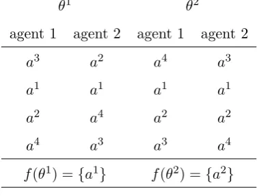
setAand the corresponding SCRf are given in Table 1.f is Pareto-inefficient
from the viewpoint of two agents because in the preference profile θ = θ2
, both agents prefer a Pareto-efficient outcomea1
∈f(θ1
): for each agentj ∈I,
a1
Pj(θ2)a2. However, since f satisfies condition µ2 (see the Appendix), it is
[image:5.595.91.281.253.396.2]Nash implementable according to Moore-Repullo’s theorem.
Table 1. A Pareto-inefficient two-agent SCR f that satisfies condition µ2.
θ1 θ2
agent 1 agent 2 agent 1 agent 2
a3 a2 a4 a3
a1 a1 a1 a1
a2 a4 a2 a2
a4 a3 a3 a4
f(θ1
) ={a1
} f(θ2
) ={a2
}
3.2 A two-agent quantum mechanism
Following Ref. [5], here we will propose a two-agent quantum mechanism to help agents combat “bad” social choice functions. According to Eq (4) in Ref. [8], two-parameter quantum strategies are drawn from the set:
ˆ
ω(θ, φ)≡
e
iφcos(θ/2) isin(θ/2)
isin(θ/2) e−iφcos(θ/2)
, (1)
ˆ
Ω ≡ {ωˆ(θ, φ) : θ ∈ [0, π], φ ∈ [0, π/2]}, ˆJ ≡ cos(γ/2) ˆI⊗n
+isin(γ/2) ˆσx
⊗n
, where γ is an entanglement measure, and ˆI ≡ ωˆ(0,0), ˆD ≡ ωˆ(π, π/2), ˆC ≡
ˆ
ω(0, π/2).
Without loss of generality, we assume:
1) Each agentj ∈I has a quantum coinj (qubit) and a classical cardj . The
basis vectors |Ci ≡ (1,0)T, |Di ≡ (0,1)T of a quantum coin denote head up
and tail up respectively.
2) Each agent j ∈ I independently performs a local unitary operation on
ψ ψ
+
ω
ω !
" #
ψ ψ$
strategic operation chosen by agent j is denoted as ˆωj ∈ Ωˆj. If ˆωj = ˆI, then
ˆ
ωj(|Ci) =|Ci, ˆωj(|Di) = |Di; If ˆωj = ˆD, then ˆωj(|Ci) =|Di, ˆωj(|Di) =|Ci.
ˆ
I denotes “Not flip”, ˆDdenotes “Flip”.
3) The two sides of a card are denoted as Side 0 and Side 1. The
informa-tion written on the Side 0 (or Side 1) of card j is denoted as card(j,0) (or
card(j,1)). A typical card of agentjis described ascj = (card(j,0), card(j,1)) ∈
Sj ×Sj, where Sj is defined in Moore-Repullo’s mechanism. The set of cj is
denoted as Cj ≡Sj×Sj.
4) There is a device that can measure the state of two quantum coins and send strategies to the designer.
Note that if ˆΩj is restricted to be {I,ˆ Dˆ}, then ˆΩj is equivalent to {Not flip,
Flip}.
Definition 1: A two-agent quantum mechanism is defined as ˆG : ˆS → A, where ˆS = ˆS1 ×Sˆ2, ˆSj = ˆΩj ×Cj (j ∈ I). ˆG can also be written as ˆG :
( ˆΩ1⊗Ωˆ2)×(C1×C2)→A, where⊗ represents tensor product.
We shall use ˆS−j to express ˆΩk×Ck (k 6= j), and thus, a strategy profile is
ˆ
s = (ˆs1,sˆ2), where ˆs1 = (ˆω1, c1) ∈Sˆ1, ˆs2 = (ˆω2, c2) ∈ Sˆ2. A Nash equilibrium
of ˆG played in a preference profile θ is a strategy profile ˆs∗
= (ˆs∗
1,sˆ
∗
2) such
that for any agent j ∈ I, ˆsj ∈ Sˆj, ˆG(ˆs∗1,ˆs
∗
2)Rj(θ) ˆG(ˆsj,ˆs∗−j). For each θ ∈ Θ,
the pair ( ˆG, θ) defines a game in normal form. Let N E( ˆG, θ)⊆ Sˆ denote the set of pure strategy Nash equilibria of the game ( ˆG, θ). Fig. 1 illustrates the
setup of the two-agent quantum mechanism ˆG. Its working steps are shown
as follows:
Step 1: The state of each quantum coin is set as |Ci. The initial state of the two quantum coins is |ψ0i=|CCi.
Step 2: Given a preference profile θ, if the two following conditions are satis-fied, goto Step 4:
1) There exists θ′
∈Θ,θ′
6
=θ such that a′
Rj(θ)a (wherea′ ∈f(θ′), a∈f(θ))
for each agent j ∈I, and a′
2) If there exists θ′′
∈ Θ, θ′′
6
= θ′
that satisfies the former condition, then
a′
Rj(θ)a′′ (where a′ ∈ f(θ′), a′′ ∈f(θ′′)) for each agent j ∈ I, and a′Pk(θ)a′′
for at least one agent k∈I.
Step 3: Each agent j sets cj = ((θj, aj, bj, nj),(θj, aj, bj, nj)) ∈ Sj ×Sj and
ˆ
ωj = ˆI. Goto Step 7.
Step 4: Each agent j sets cj = ((θ′, a′,∗,0),(θj, aj, bj, nj)). Let the two
quan-tum coins be entangled by ˆJ. |ψ1i= ˆJ|CCi.
Step 5: Each agent j independently performs a local unitary operation ˆωj on
his/her own quantum coin. |ψ2i= [ˆω1⊗ωˆ2] ˆJ|CCi.
Step 6: Let the two quantum coins be disentangled by ˆJ+
. |ψ3i = ˆJ+[ˆω1 ⊗
ˆ
ω2] ˆJ|CCi.
Step 7: The device measures the state of the two quantum coins and sends
card(j,0) (orcard(j,1)) as the strategysj to the designer if the state of
quan-tum coin j is |Ci(or |Di).
Step 8: The designer receives the overall strategys= (s1, s2) and let the final
outcome beg(s) using rules (1)-(6) of the Moore-Repullo’s mechanism. END.
Given two agents, consider the payoff to the second agent, we denote by $CC
the expected payoff when the two agents both choose ˆI(the corresponding
col-lapsed state is |CCi), and denote by $CD the expected payoff when the first
agent choose ˆI and the second agent chooses ˆD (the corresponding collapsed
state is |CDi). $DD and $DC are defined similarly. For the case of two-agent
Nash implementation, the condition λ in Ref. [5] is reformulated as the
fol-lowing condition λ′
: 1) λ′
1: Given an SCR f, a preference profile θ ∈Θ and a∈ f(θ), there exists
θ′
∈ Θ, θ′
6
=θ such that a′
Rj(θ)a (where a′ ∈ f(θ′), a ∈f(θ)) for each agent
j ∈ I, and a′
Pk(θ)a for at least one agent k ∈ I. In going from θ′ to θ both
agents encounter a preference change arounda′
. 2) λ′
2: If there exists θ
′′
∈ Θ, θ′′
6
=θ′
that satisfies λ′
1, then a
′
Rj(θ)a′′ (where
a′
∈ f(θ′
), a′′
∈ f(θ′′
)) for each agent j ∈ I, and a′
Pk(θ)a′′ for at least one
agent k ∈I. 3) λ′
3: For each agent j ∈ I, let him/her be the second agent and consider
his/her payoff, $CC >$DD.
4) λ′
4: For each agent j ∈ I, let him/her be the second agent and consider
his/her payoff, $CC >$CDcos2γ+ $DCsin2γ.
Proposition 1: For two agents, given a preference profileθ ∈Θ and a “bad”
SCR f (from the viewpoint of agents) that satisfies condition µ2, agents who
satisfies condition λ′
can combat the “bad” SCR f by virtue of a two-agent
quantum mechanism ˆG : ˆS → A, i.e., there exists a Nash equilibrium ˆs∗ ∈
N E( ˆG, θ) such that ˆG(ˆs∗
)∈/ f(θ).
The proof is straightforward according to Proposition 2 in Ref. [5]. Let us
reconsider the SCR f given in Section 3.1. Obviously, when the true
prefer-ence profile is θ2
will enter Step 4. In Step 4, two agents set c1 = ((θ 1
, a1
,∗,0),(θ2
, a2
,∗,0)),
c2 = ((θ1, a1,∗,0),(θ2, a2,∗,0)). For any agent j ∈ I, let him/her be the
second agent. Consider the payoff of the second agent, suppose $CC = 3
(the corresponding outcome is a1
), $CD = 5 (the corresponding outcome is
e(a1
, θ1
, a2
, θ2
) =a4
if j = 1, and e(a2
, θ2
, a1
, θ1
) =a3
if j = 2), $DC = 0 (the
corresponding outcome is e(a2
, θ2
, a1
, θ1
) = a3
if j = 1, and e(a1
, θ1
, a2
, θ2
) =
a4
if j = 2), $DD = 1 (the corresponding outcome is a2). Hence, condition λ′3
is satisfied, and condition λ′
4 becomes: 3 ≥5 cos
2
γ. If sin2
γ ≥ 0.4, condition
λ′
4 is satisfied.
Therefore, in the preference profile θ = θ2
, there exists a novel Nash equi-librium ˆs∗
= (ˆs∗
1,sˆ
∗
2), where ˆs
∗
1 = ˆs
∗
2 = ( ˆC,((θ 1
, a1
,∗,0),(θ2
, a2
,∗,0))), such that in Step 8 the strategy received by the designer is s = (s1, s2), where
s1 =s2 = (θ1, a1,∗,0). Consequently, ˆG(ˆs∗) = g(s) = a1 ∈/ f(θ2) = {a2}, i.e.,
the Moore and Repullo’s theorem does not hold for the “bad” social choice
rule f by virtue of the two-agent quantum mechanism ˆG.
4 A two-agent algorithmic mechanism
Following Ref. [6], in this section we will propose a two-agent algorithmic mechanism to help agents benefit from the two-agent quantum mechanism immediately.
4.1 Matrix representations of quantum states
In quantum mechanics, a quantum state can be described as a vector. For a two-level system, there are two basis vectors: (1,0)T and (0,1)T. In the
beginning, we define:
|Ci= [1,0]T, |Di= [0,1]T, |CCi= [1,0,0,0]T,
ˆ
J =
cos(γ/2) 0 0 isin(γ/2)
0 cos(γ/2) isin(γ/2) 0
0 isin(γ/2) cos(γ/2) 0
isin(γ/2) 0 0 cos(γ/2)
φ ξ
φ ξ
Forγ =π/2,
ˆ
Jπ/2 =
1
√
2
1 0 0 i
0 1 i 0
0 i 1 0
i 0 0 1
.
|ψ1i= ˆJ|CCi=
cos(γ/2) 0
0
isin(γ/2)
4.2 A two-agent algorithm
Following Ref. [6], here we will propose a two-agent version of algorithm that
simulates the quantum operations and measurements in Step 4-7 of ˆG given
in Section 3.2. The entanglement measurement γ can be simply set as its
maximumπ/2. The inputs and outputs of the two-agent algorithm are shown
in Fig. 2. The Matlab program is shown in Fig. 3(a)-(d).
Inputs:
1) (ξj, φj), j = 1,2: the parameters of agent j’s local operation ˆωj, ξj ∈
[0, π], φj ∈[0, π/2].
2)card(j,0), card(j,1)∈Sj,j = 1,2: the information written on the two sides
of agentj’s card.
Outputs:
Procedures of the algorithm:
Step 1: Reading two parameters ξj and φj from each agent j (See Fig. 3(a)).
Step 2: Computing the leftmost and rightmost columns of ˆω1 ⊗ωˆ2 (See Fig.
3(b)).
Step 3: Computing the vector representation of |ψ2i= [ˆω1⊗ωˆ2] ˆJπ/2|CCi.
Step 4: Computing the vector representation of |ψ3i= ˆJ +
π/2|ψ2i.
Step 5: Computing the probability distribution hψ3|ψ3i (See Fig. 3(c)).
Step 6: Randomly choosing a “collapsed” state from the set of all four possi-ble states{|CCi,|CDi,|DCi,|DDi}according to the probability distribution
hψ3|ψ3i.
Step 7: For each j ∈I, the algorithm sends card(j,0) (or card(j,1)) as sj to
the designer if the j-th basis vector of the “collapsed” state is |Ci (or |Di) (See Fig. 3(d)).
4.3 A two-agent version of algorithmic mechanism
Given a two-agent algorithm that simulates the quantum operations and mea-surements, the two-agent quantum mechanism ˆG: ( ˆΩ1⊗Ωˆ2)×(C1×C2)→A
can be updated to a two-agent algorithmic mechanism Ge : (Ξ1×Φ1)×(Ξ2×
Φ2)×(C1×C2)→A, where Ξ1 = Ξ2 = [0, π], Φ1 = Φ2 = [0, π/2].
We useSej to express [0, π]×[0, π/2]×Cj, andSe−j to express [0, π]×[0, π/2]×Ck
(k6=j). And thus, a strategy profile ises= (sej,se−j), wheresej = (ξj, φj, cj)∈Sej
andes−j = (ξ−j, φ−j, c−j)∈Se−j. ANash equilibriumof a two-agent algorithmic
mechanism Ge played in a preference profileθ is a strategy profilese∗
= (se∗
1,se
∗
2)
such that for any agent j ∈I, sej ∈Sej, Ge(se∗1,se
∗
2)Rj(θ)Ge(sej,se
∗ −j).
Working steps of the two-agent algorithmic mechanism Ge:
Step 1: Given an SCR f and a preference profileθ, if the two following
condi-tions are satisfied, goto Step 3: 1) There exists θ′
∈Θ,θ′
6
=θ such that a′
Rj(θ)a (wherea′ ∈f(θ′), a∈f(θ))
for each agent j ∈I, and a′
Pk(θ)a for at least one agentk ∈I;
2) If there exists θ′′
∈ Θ, θ′′
6
= θ′
that satisfies the former condition, then
a′
Rj(θ)a′′ (where a′ ∈ f(θ′), a′′ ∈f(θ′′)) for each agent j ∈ I, and a′Pk(θ)a′′
for at least one agent k∈I.
Step 2: Each agent j sets card(j,0) = (θj, aj, bj, nj) and sends card(j,0) as
the strategy sj to the designer. Goto Step 5.
Step 3: Each agentjsetscard(j,0) = (θ′
, a′
,∗,0) andcard(j,1) = (θj, aj, bj, nj),
then submitsξj,φj, card(j,0) and card(j,1) to the two-agent algorithm.
Step 4: The two-agent algorithm runs in a computer and outputs strategiess1
and s2 to the designer.
outcome beg(s) using rules (1)-(6) of the Moore-Repullo’s mechanism. END.
4.4 New result for two-agent Nash implementation
As we have seen, in the two-agent algorithmic mechanismGe, the entanglement
measurement γ is reduced to its maximum π/2. Hence, condition λ′
shall be revised as λ′π/2
, where λ′1π/2, λ
′π/2
2 and λ
′π/2
3 are the same as λ
′
1, λ
′
2 and λ
′
3
respectively. λ′4π/2 is revised as follows:
λ′4π/2: For each agent j ∈ I, let him/her be the second agent and consider
his/her payoff, $CC >$DC.
Proposition 2: For two agents, given a preference profileθ∈Θ and an SCR
f that satisfies condition µ2: 1) If condition λ′π/2
is satisfied, then f is not Nash implementable.
2) If condition λ′π/2
is not satisfied, then f is Nash implementable. Put
dif-ferently, the sufficient and necessary conditions for Nash implementation with two agents are updated as condition µ2 and no-λ′π/2
.
The proof is straightforward according to Proposition 1 in Ref. [6]. Obviously,
the two-agent algorithmic mechanism proposed here is a completely “classical”
one that can be run in a computer.
5 Conclusions
This paper generalizes the quantum and algorithmic mechanisms in Refs. [5,6] to the case of two-agent Nash implementation. Although Moore and Repullo used the phrase “a full characterization” to claim that the problem of two-agent Nash implementation had been completely solved, we argue that there exists a new result as Proposition 2 specifies.
Appendix
Consider the SCR f specified by Table 1. I = {1,2}, A = {a1
, a2
, a3
, a4
},
Θ = {θ1
, θ2
}. Let B = A and Cj(a, θ) = Lj(a, θ) for each j ∈ I, θ ∈ Θ,
a∈f(θ), i.e.,
C1(a 1
, θ1
) =L1(a 1
, θ1
) = {a1
, a2
, a4
}, C2(a
1
, θ1
) =L2(a 1
, θ1
) = {a1
, a3
, a4
}, C1(a
2
, θ2
) =L1(a 2
, θ2
) = {a2
, a3
}, C2(a
2
, θ2
) =L2(a 2
, θ2
) = {a2
, a4
}.
Obviously,
a1
∈M1(C1(a 1
, θ1
), θ1
) ={a1
}, a1
∈M2(C2(a 1
, θ1
), θ1
) ={a1
}, a2
∈M1(C1(a 2
, θ2
), θ2
) ={a2
}, a2
∈M2(C2(a 2
, θ2
), θ2
) ={a2
}.
For each 4-tuple (a, θ, a′
, θ′
)∈A×Θ×A×Θ, let
e(a1
, θ1
, a1
, θ1
) = a1
∈C1(a 1
, θ1
)∩C2(a 1
, θ1
) = {a1
, a4
}, e(a1
, θ1
, a2
, θ2
) = a4
∈C1(a 1
, θ1
)∩C2(a 2
, θ2
) = {a2
, a4
}, e(a2
, θ2
, a1
, θ1
) = a3
∈C1(a 2
, θ2
)∩C2(a 1
, θ1
) = {a3
}, e(a2, θ2, a2, θ2) = a2 ∈C1(a
2
, θ2)∩C2(a 2
, θ2) = {a2}.
Case 1): Consider θ∗
=θ1
,f(θ∗
) ={a1
}.
For rule (i):
M1(C1(a 1
, θ1
), θ∗
)∩M2(C2(a 1
, θ1
), θ∗
) = {a1
} ∩ {a1
}={a1
}, M1(C1(a
2
, θ2
), θ∗
)∩M2(C2(a 2
, θ2
), θ∗
) = {a3
} ∩ {a2
}=φ.
Hence, rule (i) is satisfied.
For rule (ii):
M1(C1(a 1
, θ1
), θ∗
)∩M2(B, θ
∗
) ={a1
} ∩ {a2
}=φ, M1(C1(a
2
, θ2
), θ∗
)∩M2(B, θ
∗
) ={a3
} ∩ {a2
}=φ, M2(C2(a
1
, θ1
), θ∗
)∩M1(B, θ
∗
) ={a1
} ∩ {a3
}=φ, M2(C2(a
2
, θ2
), θ∗
)∩M1(B, θ
∗
) ={a2
} ∩ {a3
}=φ.
For rule (iii):
M1(B, θ
∗
)∩M2(B, θ
∗
) = {a3
} ∩ {a2
}=φ.
Hence, rule (iii) is satisfied.
For rule (iv):
e(a1
, θ1
, a1
, θ1
) =a1
, M1(C1(a 1
, θ1
), θ∗
)∩M2(C2(a 1
, θ1
), θ∗
) ={a1
} ∩ {a1
}={a1
}, e(a1
, θ1
, a2
, θ2
) =a4
, M1(C1(a 1
, θ1
), θ∗
)∩M2(C2(a 2
, θ2
), θ∗
) ={a1
} ∩ {a2
}=φ, e(a2
, θ2
, a1
, θ1
) =a3
, M1(C1(a 2
, θ2
), θ∗
)∩M2(C2(a 1
, θ1
), θ∗
) ={a3
} ∩ {a1
}=φ, e(a2
, θ2
, a2
, θ2
) =a2
, M1(C1(a 2
, θ2
), θ∗
)∩M2(C2(a 2
, θ2
), θ∗
) ={a3
} ∩ {a2
}=φ.
Hence, rule (iv) is satisfied.
Case 2): Consider θ∗
=θ2
,f(θ∗
) ={a2
}.
For rule (i):
M1(C1(a 1
, θ1
), θ∗
)∩M2(C2(a 1
, θ1
), θ∗
) = {a4
} ∩ {a3
}=φ, M1(C1(a
2
, θ2
), θ∗
)∩M2(C2(a 2
, θ2
), θ∗
) = {a2
} ∩ {a2
}={a2
}.
Hence, rule (i) is satisfied.
For rule (ii):
M1(C1(a 1
, θ1
), θ∗
)∩M2(B, θ
∗
) ={a4
} ∩ {a3
}=φ, M1(C1(a
2
, θ2
), θ∗
)∩M2(B, θ
∗
) ={a2
} ∩ {a3
}=φ, M2(C2(a
1
, θ1
), θ∗
)∩M1(B, θ
∗
) ={a3
} ∩ {a4
}=φ, M2(C2(a
2
, θ2
), θ∗
)∩M1(B, θ
∗
) ={a2
} ∩ {a4
}=φ.
Hence, rule (ii) is satisfied.
For rule (iii):
M1(B, θ
∗
)∩M2(B, θ
∗
) = {a4
} ∩ {a3
}=φ.
Hence, rule (iii) is satisfied.
For rule (iv):
e(a1
, θ1
, a1
, θ1
) =a1
, M1(C1(a 1
, θ1
), θ∗
)∩M2(C2(a 1
, θ1
), θ∗
) ={a4
} ∩ {a3
}=φ, e(a1
, θ1
, a2
, θ2
) =a4
, M1(C1(a 1
, θ1
), θ∗
)∩M2(C2(a 2
, θ2
), θ∗
) ={a4
} ∩ {a2
}=φ, e(a2
, θ2
, a1
, θ1
) =a3
, M1(C1(a 2
, θ2
), θ∗
)∩M2(C2(a 1
, θ1
), θ∗
) ={a2
} ∩ {a3
}=φ, e(a2
, θ2
, a2
, θ2
) =a2
, M1(C1(a 2
, θ2
), θ∗
)∩M2(C2(a 2
, θ2
), θ∗
) ={a2
} ∩ {a2
}={a2
}.
To sum up, the SCR f given in Table 1 satisfies condition µ2. Therefore,
ac-cording to Moore-Repullo’s theorem, it should be Nash implementable.
How-ever, as shown in Section 3 and 4, when conditionλ′
is satisfied, neither in the
quantum world nor in the macro world will the SCRf be Nash implementable.
Acknowledgments
The author is very grateful to Ms. Fang Chen, Hanyue Wu (Apple), Hanxing
Wu (Lily) and Hanchen Wu (Cindy) for their great support.
References
[1] E. Maskin, Nash equilibrium and welfare optimality, Rev. Econom. Stud. 66
(1999) 23-38.
[2] J. Moore and R. Repullo, Nash implementation: a full characterization,
Econometrica 58(1990) 1083-1099.
[3] B. Dutta and A. Sen, A necessary and sufficient condition for two-person Nash implementation,Rev. Econom. Stud.58 (1991) 121-128.
[4] F. Busutto and G. Codognato, Reconsidering two-agent Nash implementation,
Social Choice and Welfare 32(2009) 171-179.
[5] H. Wu, Quantum mechanism helps agents combat “bad” social choice rules.
International Journal of Quantum Information, 2010 (accepted). http://arxiv.org/abs/1002.4294
[6] H. Wu, On amending the sufficient conditions for Nash implementation.
Theoretical Computer Science, 2011 (submitted). http://arxiv.org/abs/1004.5327
[7] T.D. Ladd, F. Jelezko, R. Laflamme, Y. Nakamura, C. Monroe and J.L. O’Brien, Quantum computers,Nature,464 (2010) 45-53.
%************************************************************ % A two-agent algorithm
%************************************************************
% Defining the array of xi=zeros(2,1);
phi=zeros(2,1);
% Reading agent 1's parameters . For example, xi(1)=0;
phi(1)=pi/2;
% Reading agent 2's parameters . For example, xi(2)=0;
phi(2)=pi/2;
π ω
ω = =
π ω
ω = =
=
φ ξ
φ ξ
φ ξ
ξ φ =
% Defining two 2*2 matrices A and B A=zeros(2,2);
B=zeros(2,2);
% Let A represents the local operation of agent 1. A(1,1)=exp(i*phi(1))*cos(xi(1)/2);
A(1,2)=i*sin(xi(1)/2); A(2,1)=A(1,2);
A(2,2)=exp(-i*phi(1))*cos(xi(1)/2);
% Let B represents the local operation of agent 2. B(1,1)=exp(i*phi(2))*cos(xi(2)/2);
B(1,2)=i*sin(xi(2)/2); B(2,1)=B(1,2);
B(2,2)=exp(-i*phi(2))*cos(xi(2)/2);
% Computing the leftmost and rightmost columns of C=zeros(4, 2);
for row=1 : 2
C((row-1)*2+1, 1) = A(row,1) * B(1,1); C((row-1)*2+2, 1) = A(row,1) * B(2,1); C((row-1)*2+1, 2) = A(row,2) * B(1,2); C((row-1)*2+2, 2) = A(row,2) * B(2,2); end
A=C;
% Now the matrix A contains the leftmost and rightmost columns of
ω
ω ω ⊗
ω
ω ω ⊗
ω
% Computing psi2=zeros(4,1); for row=1 : 4
psi2(row)=(A(row,1)+A(row,2)*i)/sqrt(2); end
% Computing psi3=zeros(4,1); for row=1 : 4
psi3(row)=(psi2(row) - i*psi2(5-row))/sqrt(2); end
% Computing the probability distribution distribution=psi3.*conj(psi3);
distribution=distribution./sum(distribution);
ψ ψ = π+
π
ω ω
ψ = ⊗
ψ ψ
ψ ψ ψ ψ
% Randomly choosing a “collapsed” state according to the probability distribution random_number=rand;
temp=0; for index=1: 4
temp = temp + distribution(index); if temp >= random_number
break; end end
% indexstr: a binary representation of the index of the collapsed state % ‘0’ stands for , ‘1’ stands for
indexstr=dec2bin(index-1); sizeofindexstr=size(indexstr);
% Defining an array of strategies for two agents strategy=cell(2,1);
% For each agent , the algorithm generates the strategy for index=1 : 2 - sizeofindexstr(2)
strategy{index,1}=strcat('card(',int2str(index),',0)'); end
for index=1 : sizeofindexstr(2)
if indexstr(index)=='0' % Note: ‘0’ stands for
strategy{2-sizeofindexstr(2)+index,1}=strcat('card(',int2str(2-sizeofindexstr(2)+index),',0)'); else
strategy{2-sizeofindexstr(2)+index,1}=strcat('card(',int2str(2-sizeofindexstr(2)+index),',1)'); end
end
% The algorithm outputs the strategies to the designer for index=1:2
disp(strategy(index)); end
ψ ψ
∈