Feature Selection for Time Series Modeling

(1)

Feature Selection for Time Series Modeling

*

Qing-Guo Wang, Xian Li, Qin Qin, Nguyen Gia Huy

Department of Electrical and Computer Engineering, National University of Singapore, Singapore. Email: [email protected], [email protected], [email protected]

Received March 18th_{, 2013; revised April 18}th_{, 2013; accepted April 25}th_{, 2013}

Copyright © 2013 Qing-Guo Wang et al. This is an open access article distributed under the Creative Commons Attribution License, which permits unrestricted use, distribution, and reproduction in any medium, provided the original work is properly cited.

ABSTRACT

In machine learning, selecting useful features and rejecting redundant features is the prerequisite for better modeling and prediction. In this paper, we first study representative feature selection methods based on correlation analysis, and demonstrate that they do not work well for time series though they can work well for static systems. Then, theoretical analysis for linear time series is carried out to show why they fail. Based on these observations, we propose a new cor-relation-based feature selection method. Our main idea is that the features highly correlated with progressive response while lowly correlated with other features should be selected, and for groups of selected features with similar residuals, the one with a smaller number of features should be selected. For linear and nonlinear time series, the proposed method yields high accuracy in both feature selection and feature rejection.

Keywords: Time Series; Feature Selection; Correlation Analysis; Modeling; Nonlinear Systems

1. Introduction

In machine learning, the models quality depends much on features used. Often, one faces problems of lacking useful features and/or of redundant features, causing poor modeling and prediction performance. For better modeling, we need to include high predictive capability features and exclude low predictive capability or redundant features from the original group of features. Good feature selection can increase the modeling efficiency and is the prerequisite for subsequent works. Hence, identifying a series of representative features has become a central problem. In general, features reduction, consists of feature selection [1] and feature extraction [2]. The former one tries to find a subset which fit the model best from original features set, while the latter one attempts to transform the original high dimension features space into a low one. The features selection can be further divided into two categories: filters [2] and wrappers [3].

Time series [4] is a collection of observations taken sequentially in time, and occurs in many fields, e.g. the

stock price in successive minutes [5], the indoor tem- perature in successive hours, etc. In this paper, we ad- dress feature selection for time series. To this end, many methods of feature selection have been reported in the literature. However, none of them can always produce the good performance. In this regard, we first conduct comparative study of several typical correlation based methods of feature selection, and find that they do not work well for time series though they can work well for static systems. This motivates us to provide better sche- mes for feature selection. Then, theoretical analysis for linear time series is carried out to show why they fail. Based on these observations, we propose a new correlation-based feature selection method. Our main idea is that the features highly correlated with progressive response while lowly correlated with other features should be selected, and for groups of selected features with similar residuals, the one with a smaller number of features should be selected. For linear and nonlinear time series, the proposed method yields high accuracy in both feature selection and feature rejection.

The rest of this paper is organized as follows. The feature selection methods are presented in Section 2. In Section 3, we describe the data sets obtained and simulation designs. The results and discussions are given in Section 4. Finally, conclusions are drawn in Section 5.

*_{This research is funded by the Republic of Singapores National}

(2)

2. Feature Selection

2.1. Linear Regression Method

In linear regression method [6], suppose that the response

 

y t is related to the feature x t

 

in a linear fashion,

 

1 1

, 1, 2, , ,

r m

i i r j j i j

y k x k  _ k k N

 









  (1)

where j are m random variables with uniform distribution on interval



b b,



, independent of each other,

and added into x t

 

to test for effectiveness of this fea-

ture selection method. These equations for all k are

integrated to form the matrix equation, ,

Y X (2)

where

   

1 , 2 , ,

 

T,

Y  _y y  y N _ (3)

 

1 1

1 1 1 1

,

r m

x x

X

x N x N N N

                         (4)



1, 2, , , 1, 2, ,



.

T r r r r m

     _  _  _ (5)

It is solved by the linear least squares method [7] to find weights . We find the maximum absolute value of last m weights,



1



max

max , , if > 0 .

0 if 0

r r m m

m    _{ }      (6)

The feature xi is retained in the selected feature group if i >_max, or discarded otherwise.

2.2. Linear Correlation Method

Pearson product-moment correlation coefficient [8] is a measure of the linear dependence of two variables X

and Y, giving a value between −1 and 1 inclusive. It is

usually estimated by















1 , 2 2 1 1 , n i i i X Y n n i i i i

X X Y Y

        



(7)

based on a sample of paired data



X Yi, i



. Similarly to

the linear regression method, we add m random variables

with uniform distribution on interval



b b,



, independent of each other, and added into x t

 

to test for

effectiveness of this feature selection method. Linear correlation coefficients i between response y t

 

and each feature x ti

 

are calculated, and the maxi-

mum absolute value of the last r ones is determined,



1



max

max , , if > 0 .

0 if 0

r r m m m            (8)

The feature x ti

 

is retained in the selected feature

group if i >_max, i.e. x ti

 

is more correlated to the

response than the random variables. Otherwise, x ti

 

is

discarded.

2.3. Spearsmans Correlation Method

It is well known that the relationships between features and the response could be nonlinear. The linear correlation coefficient captures the linear relation only, and thus is not accurate in the nonlinear case, which calls for nonlinear correlation coefficient method. The simplest nonlinear correlation coefficient is the Spearmans rank correlation coefficient, and it is more appropriate when the data points seem to follow a curve instead of a straight line, and is less sensitive to the effects of outliers. Spearmans rank correlation coefficient is a measure of statistical dependence between 2 variables, and is defined as the Pearson correlation coefficient between the ranked variables [9]. Given n raw data points



X Yi, i



, Xi are ranked with ai such that the largest value has rank 1, the second largest value rank 2, etc. whereas Yi are similarly ranked with bi. Spearmans rank correlation coefficient of Xi and Yi is Pearson correlation coefficient calculated from ai and bi. The efficient way to calculate Spearmans rank correlation coefficient is to use









2 2 6 1 . 1 i i s a b n n     



₍₉₎

The feature selection based Spearmans rank correlation coefficient follows its linear counterpart by re- placing the linear correlation coefficients by Spearmans rank correlation coefficient.

2.4. Local Learning Method

A new algorithm, called “Local Learning Based Feature Selection for High Dimensional Data Analysis of feature selection”, was proposed by Sun et al. [10]. Its core idea

is that an arbitrarily complicated nonlinear problem can be decomposed into a series of local linear problems based on local learning and then the feature relevance is learned globally. Their method does not make any assumption on the data distribution, and is capable of selecting useful features successfully from a large number of features that are irrelevant. Its flowchart is shown as follows.

Input: Data





   





 

1

D , N J 1

i

x i y i R



    , kernel

(3)

Output: Feature weights w.

1. Initiation: Set  0 _1, _1.

w  t

2. Repeat:

a) Compute



   

 1



d , t , ,

i j

x i x j w  x x D

b) Compute



 



 



 t 1



NM

P P x j NM x i w  and

 



 



 



t 1



NH

P P x j NH x i w  with equations,

   





   



w



,

NM n

n M_n w

k x i x j

P j M

k x i x n

     



and

   





   



w



,

NH n

n Hn w

k x i x j

P j H

k x i x n





  





c) Solve for v through gradient descent using the

update rule,

 





 





  2 2 1 2 exp 1 1 exp ,1

N _j _i j

i i _j _i

j t

j j

z j

v v z v

z j

w v j J

      _      _  _       



d) t t 1

3. Until:  t  t1 _{< .}

w w  

4.  t.

ww

In this algorithm, x i

 

is the feature vector, y i

 

is

the label corresponding to x i

 

, and d() stands for the

Manhattan distance of u



u u1, , ,2  un



,



1, , ,2 n



v v v  v .

1

n i i i

d u v





 (10)

2.5. 2D-Correlation Method

The correlation methods mentioned above only consider correlation from features to response. It tends to select redundant features if these features are all highly related to response but they are mutually correlated too. To select a set of features as good and few as possible for learning task, one must take into consideration possible interdependencies between the features as well. As a trade-off between the complexity of the selection process and the quality of the selected feature set, a pair wise selection strategy has been recently suggested [11]. This method assumes that a feature is irrelevant if it is uncorrelated with response, otherwise it is useful, and the feature is redundant if a feature is highly correlated with other features.

In this paper, we propose some modifications. Firstly, we use the rank correlation coefficient instead as it can capture nonlinear relation and is computational efficient.

Secondly, we compare correlation from real features with those from pure noises, and retain those features only when they are more relevant than noises. Thirdly, we introduce tuning parameters to allow the users to fit to specific situations. Thus, the main idea of this modified method is to check first whether the features are correlated in linear or nonlinear way to each other. If the correlation coefficients between a feature and other features exceed the correlation coefficient between this feature and response by some extent, it means that this feature is not useful, and its information can be gained from high correlated other features. The detailed procedure is as follows,

1. Initialization:

a) Define the feature sets: Set Fo as the original set of n features and the selected feature set Fs as empty set.

b) Select the first feature: compute the rank correlation coefficient 



x y_i,



between the feature x_i and

the response y . Then include the feature with the

largest 



x yi,



as the first selected feature in Fs and exclude it from Fo.

c) Remove noisy features: compute the rank correlation coefficient  



i,y



between noise i and the response y, where i1, 2, , m. Set the default m as 20.

Let the standard deviation of these m coefficients be .

Take xi away from Fo, if xi be in Fo such that



x yi,



<

 , where  is the threshold ratio.

2. Search for relevant features, repeat until no feature is produced from (b) below.

a) Compute the rank correlation coefficient 



x xi, j



for each pair of variables



x x_i, _j



with xiFo and

j s

x F .

b) Select the next feature: choose feature xiFo as the one that maximizes









, , i i j j

n x y

n n x x

 





, subject to









, > , i i j j

n x y

n n x x



 





, where  is the threshold

ratio. Move xi from Fo into Fs.

3. Output the set Fs as the selected features.

It will be seen from our simulation study below that correlation based methods work badly for time series in general. The best one, the 2D-correlation method, is able to reject irrelevant features but unable to select minimum number of relevant features. We will find causes of their failure through theoretical analysis in the next section.

3. Theoretical Analysis and Progressive

Correlation Method

(4)

which is described by

 

1



1



p



  

,

x t  x t    x tp  t (11)

where

 



 

t is a purely random process with zero

mean and variance 2

z

 . Assume this process is sta- tionary. Then multiply through (11) by x t



k



, take

expectations, and divide 2

x

 to get

 









1

< 0

1 0 ,

1 p 1

k k

k k p k

         _   _{  } _ _   (12)

where 

 

k is the correlation coefficients of

 

x t

 

and



x t



k





[4]. This holds true, independent of the

initial condition and variance of

 



 

t . For p3, (12)

becomes

 













1 2 3

2

2 1 3 3

2 2

1 1 3 2 2

2

2 1 3 3

1 2 3

0 1 1

1

2 1

1 2 3 , 3

k k k k k

                             _  _           _  _ _ _          (13)

It is shown in Figure 1 for 12.9979,2 2.9967, 3 0.9988

  .

If the 2D-correlation method is applied to the above case, we find that there is low efficiency in selecting useful features. Suppose that the feature with time lag 1,



1



x t , is selected, features with time lags 2, x t



2



,

and 3, x t



3



, should be considered in the subsequent

steps. For system in (11) with p3, it follows from (13)

and Figure 1 that features, x t



2



and x t



3



, have

higher correlation with selected feature, x t



1



, than

that with response, x t

 

, and thus are not selected. In

general, it is observed that though x t



k



, >k p, are

[image:4.595.68.277.559.717.2]

redundant, each of them have significant correlation with response and their values are not necessarily smaller than

Figure 1. Correlation coefficient for p = 3.

those of x t



k



,k p. Besides, they are not nece-

ssarily smaller than their own mutual correlations. Thus, the methods mentioned above fail in general.

To overcome the drawbacks in the above correlation methods, we propose the progressive correlation method as follows. Select xi , if correlation of xi and



yixi



decreases significantly with that of xi and y, no longer solely based on single correlation of x_i with y.

Further, we also use the correlation of xj with



yixi



when we consider xj after xi is selected. In this new method, we favor the feature with least time lags when several features with similar relative correlation coefficients exist. And if several groups of selected features have similar modeling residuals, we favor the one with a smaller number of features. The detailed procedure is as follows,

1. Initialization:

a) Define the feature sets: Set Fo as the original set of n features and the selected feature set Fs as empty set.

b) Select the first feature: compute the rank correlation coefficient 



x yi,



between the feature xi and response y. Then find the features which satisfy





















max , ,

max ,

i i i

i i

x y x y

x y

 

 



 and select among them,

one with the least time lag. Include it in Fs and exclude it from Fo.

c) Remove noisy features: compute the rank correlation coefficient  



i,y



between noise i and the response y, where i1, 2, , m. Set the default m as

20. Let the standard deviation of these m coefficients

be  . Let xi in Fo be such that 



x yi,



<, where  is the threshold ratio. Take xi away from

o

F .

2. Select feature progressively, repeat until the root mean square error of modelled system stops decreasing or there is no feature in Fo:

a) Learn a model with the selected features and response, and calculate the model residual series e.

b) Calculate rank correlation coefficients 



x ei,



with xiFo. Then calculate relative correlation coefficients with













, , , i r i i j j

n x e

x e

n n x x

 

 





.

c) Select the feature xi which satisfies

















max , ,

max ,

r i i

i

x e x e

x e

 

 



 with minimal time lag

(5)

d) Update the response with the model residual e.

3. Varying  to different values, and redo step 1. and 2., several groups of features are selected. For those have similar small modelling residuals, we select the one with smaller number of features and less time lag as final selected features.

4. Output the set Fs as the selected features.

4. Simulation Data and Design

For testing feature selection on time series, we construct two dynamic systems. The first one is linear system and described by

 

1



1



2



2



3



3

  

,

u t u t  u t  u t  t (14)

where  is white noise with uniform distribution on interval



b b,



. Coefficients are set as ₁2.9979,

2 2.9967,

   ₃0.9988, and the initial conditions are set to be u

 

0 10, 1u

 

10,u

 

2 10.002. Then

the equation gives us a stable system and the response is shown in Figure 2.

The second system is nonlinear and described by

 







  



















 

1 2 3 4

5 6

min 1 max 1 2 , , log 3 cos 4 ,

u t

u t u t u t

u t u t t

   

  

      

    

(15) where  is white noise with uniform distribution on interval



b b,



. At last, we set ₁ 2 1, ₂ 1,

3 10, 4 10 2 2 , 5 10, 6 10

         and the initial conditions are set to be u

 

0 10, 1u

 

10,u

 

2 10,

 

3 10

u  . Its response is shown in Figure 3. The model without the last three terms in the right hand side is cited from [12], which represents some economic model with cycles.

As our objective is to predict the system response change based on the past observations, we form the features x t

 

as

 



1 ,

 

2 , ,







,

x t _u t u t  u tr _ (16)

and the response y t

 

for regression as

 

  

1 .



y t u t u t (17)

For classification, we define the label for each feature vector from its corresponding response as follows (0% threshold)

 



  



  







1, if 1 > 0 . 0, if 1 < 0

u t u t

y t

u t u t

  

  

 

 (18)

The data set for learning is thus formed by

 

   



, , 1, ,



[image:5.595.306.540.84.435.2]

Z  z t _x t y t _tr r  n with the data

Figure 2. The linear dynamic system.

Figure 3. The nonlinear dynamic system.

size equal to N   n r 1.

Sometimes, one may be interested in large changes only. Then, one can filter the response with some threshold d : a data point in the original data set is kept in

the filtered data set for regression if

 



  

1 >





1



y t  u t u t d u t . The other data

points are discarded. The size of the filtered data set will thus be usually reduced, depending on the actual response. The filtered data set for classification is obtained by using the same label definition before.

Equations (16) to (18) are used to generate the following data sets for both linear and nonlinear systems labeled by

r = 2, 4, 8, 10 d = 0, 0.01 m = 0, 3 b = 0.01, 0.1, 1

The Noise-to-Signal Ratio (NSR) is obtained by

 

2

2 .

t NSR

u t







(19)

5. Simulation Results

[image:5.595.310.540.85.241.2]

(6)

existing methods, respectively, and make a comparison. Then, we present results of the proposed methods (2D- Correlation Method and Progressive Correlation Me- thod).

5.1. Comparison of First Four Methods

Comparisons are made firstly based on the performance for different values of the magnitude of random variables added



b0.01, 0.1,1



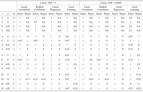
. After that, normalization is

[image:6.595.58.540.429.739.2]

applied to both the feature and response, and perfor- mances of the first four methods are then compared in Table 1 to Table 9, respectively.

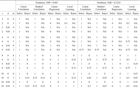
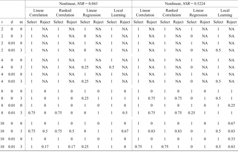
From the results above, we can conclude that the magnitude of random variables added does not have any significant effect on the performance of the 4 methods: linear regression, linear correlation coefficient, rank correlation coefficient, and local learning method. There are some cases when the performance is affected, for example when Spearmans rank correlation method was applied to nonlinear system with NSR = 0.5224 and r =

10, d = 0.01, m = 3, the rejection rate for b = 0.01 is 0.83,

for b = 0.1 is 0.67, and for b = 1 is 1. However, in the

majority of the cases, the rejection rate and selection rate are about the same. This might be because the random features which were added do not have any correlation with the response, and thus their correlation coefficient

with respect to the response is close to 0. When the magnitude of random variables is increased, the correlation coefficient might be increased, but the change is not very big due to the random nature of these variables. There- fore, the threshold level might not have increased by so much, and the performance level is roughly the same.

Overall, Dr. Suns method of feature selection based on local learning seems to give the best result. In most cases, it is able to remove at least some, if not the majority of the irrelevant features. However, not all of the relevant features were selected; and it fails altogether in a few cases. Nevertheless, it still gives better result than linear correlation coefficient, rank correlation coefficient, and linear regression, which tends to select most of the features, regardless of whether they are relevant.

5.2. 2D-Correlation Method

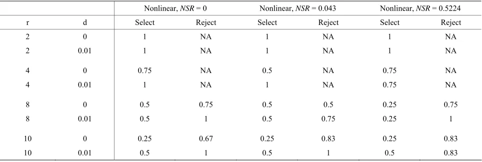
In the simulation of correlation method, we set the threshold  as 1.5 and the parameter  as 0.5. In our ex- periments, it indicates that the magnitude of added random variables do not affect the performance significantly, and is set as fixed one [−1, 1]. The simulation results are shown in Tables 10 and 11.

In terms of feature rejection, we observe that the correlation method yields quite positive results. In most of the cases, this method is able to eliminate most of the irre-

Table 1. Performance when b = 0.01 (Part 1).

Linear, NSR = 0 Linear, NSR = 0.8649

Linear Correlation

Ranked Correlation

Linear Regression

Local Learning

Linear Correlation

Ranked Correlation

Linear Regression

Local Learning r d m Select Reject Select Reject Select Reject Select Reject Select Reject Select Reject Select Reject Select Reject

2 0 0 1 NA 1 NA 1 NA 1 NA 1 NA 1 NA 1 NA 0.5 NA

2 0 3 1 NA 0.5 NA 1 NA 1 NA 1 NA 1 NA 1 NA 1 NA

2 0.01 0 1 NA 1 NA 1 NA 1 NA 1 NA 1 NA 1 NA 0.5 NA

4 0 0 1 0 1 0 1 0 0.67 1 1 0 1 0 1 0 0.67 1

4 0 3 0.67 1 0.67 1 1 0 0.67 1 1 0 1 0 1 0 1 1

4 0.01 0 1 0 1 0 1 0 1 0 1 0 1 0 1 0 0.33 0

4 0.01 3 1 0 1 0 1 0 0.33 0 1 0 1 0 1 0 0.33 0

8 0 0 1 0 1 0 1 0 0.67 1 1 0 1 0 1 0 1 0.8

8 0 3 0.67 1 0 1 1 0 0.33 1 1 0.8 0.67 1 1 0 0.33 1

8 0.01 0 1 0 1 0 1 0 1 0.6 1 0 1 0 1 0 1 0.2

8 0.01 3 1 0 1 0 1 0 1 0 1 0 1 0 1 0 1 0

10 0 0 1 0 1 0 1 0 0.67 1 1 0 1 0 1 0 1 0.14

10 0 3 1 0.57 0.33 0.43 1 0 0.67 1 1 0.43 1 0.43 1 0 1 0.29

10 0.01 0 1 0 1 0 1 0 1 0.29 1 0 1 0 1 0 0 0

(7)

[image:7.595.57.541.104.416.2]

Linear, NSR = 13.7462 Nonlinear, NSR = 0

Linear Correlation

Ranked Correlation

Linear Regression

Local Learning

Linear Correlation

Ranked Correlation

Linear Regression

2 0 0 1 NA 1 NA 1 NA 0.5 NA 1 NA 1 NA 1 NA 1 NA

2 0 3 0.5 NA 0 NA 1 NA 0 NA 1 NA 1 NA 0 NA 1 NA

2 0.01 0 1 NA 1 NA 1 NA 1 NA 1 NA 1 NA 1 NA 1 NA

2 0.01 3 0.5 NA 0.5 NA 1 NA 0 NA 1 NA 1 NA 0 NA 1 NA

4 0 0 1 0 1 0 1 0 0 1 1 NA 1 NA 1 NA 1 NA

4 0 3 0.67 0 0.33 1 1 0 0 1 1 NA 1 NA 0 NA 1 NA

4 0.01 0 1 0 1 0 1 0 0 0 1 NA 1 NA 1 NA 0.75 NA

4 0.01 3 0.67 0 0.67 0 1 0 0 0 1 NA 1 NA 0 NA 1 NA

8 0 0 1 0 1 0 1 0 0.67 0.6 1 0 1 0 1 0 1 0

8 0 3 0.33 0 0 0.2 1 0 0.67 0.6 1 0 1 0 0 1 1 1

8 0.01 0 1 0 1 0 1 0 0.67 0 1 0 1 0 1 0 1 0

8 0.01 3 0.67 0 0.33 0 1 0 0 0.4 1 0 1 0 0 1 1 0.25

10 0 0 1 0 1 0 1 0 1 0.14 1 0 1 0 1 0 1 0

10 0 3 0 0 1 0 1 0 0.67 0.29 1 0.17 1 0.17 0 1 1 1

10 0.01 0 1 0 1 0 1 0 0 0 1 0 1 0 1 0 1 0

10 0.01 3 0 0 0 0 1 0.14 0.67 0 1 0.33 1 0.17 0 1 1 0

Nonlinear, NSR = 0.043 Nonlinear, NSR = 0.5224

Linear Correlation

Ranked Correlation

Linear Regression

Local Learning

Linear Correlation

Ranked Correlation

Linear Regression

2 0 0 1 NA 1 NA 1 NA 1 NA 1 NA 1 NA 1 NA 1 NA

4 0.01 3 1 NA 0.75 NA 0 NA 1 NA 0.75 NA 1 NA 0 NA 0.75 NA

8 0 0 1 0 1 0 1 0 1 0 1 0 1 0 1 0 1 1

8 0 3 1 0 1 0 0 1 1 1 1 0.75 1 0.75 0 1 1 1

8 0.01 0 1 0 1 0 1 0 1 0 1 0 1 0 1 0 1 0.25

8 0.01 3 1 0 1 0 0 1 1 0 1 0.75 1 0.75 0 1 1 1

10 0 0 1 0 1 0 1 0 1 0.25 1 0 1 0 1 0 1 0.67

10 0 3 1 0.17 1 0.17 0 1 1 1 1 0.67 1 0.67 0 1 0.75 0.83

10 0.01 0 1 0 1 0 1 0 1 0 1 0 1 0 1 0 1 0.33

[image:7.595.59.538.431.734.2]

(8)

[image:8.595.59.541.100.405.2]

Linear Correlation

Ranked Correlation

Linear Regression

Local Learning

Linear Correlation

Ranked Correlation

Linear Regression

2 0.01 3 1 NA 1 NA 1 NA 0.5 NA 1 NA 1 NA 1 NA 0 NA

4 0 0 1 0 1 0 1 0 0.67 1 1 0 1 0 1 0 0.67 1

4 0 3 0.67 1 0 1 1 0 0.67 1 1 0 1 0 1 0 0.67 1

4 0.01 0 1 0 1 0 1 0 1 0 1 0 1 0 1 0 0.33 0

4 0.01 3 1 0 1 0 1 0 0 0 1 0 1 0 1 0 0.33 0

8 0 0 1 0 1 0 1 0 0.67 1 1 0 1 0 1 0 1 0.8

8 0 3 1 0.8 0.33 0.6 1 0 0.67 1 1 0.4 1 0.6 1 0 1 0.8

8 0.01 0 1 0 1 0 1 0 1 0.6 1 0 1 0 1 0 1 0.2

8 0.01 3 1 0 1 0 1 0 1 0.2 1 0 1 0 1 0 1 0

10 0 0 1 0 1 0 1 0 0.67 1 1 0 1 0 1 0 1 0.14

10 0 3 0.67 0.71 0 0.57 1 0 0.33 1 1 0.14 1 0.14 1 0 1 0.43

10 0.01 0 1 0 1 0 1 0 1 0.29 1 0 1 0 1 0 0 0

[image:8.595.61.538.432.738.2]

10 0.01 3 1 0 1 0 1 0 1 0.14 1 0 1 0 1 0 0.33 0.29

Linear Correlation

Ranked Correlation

Linear Regression

Local Learning

Linear Correlation

Ranked Correlation

Linear Regression

2 0 3 0.5 NA 0.5 NA 1 NA 0 NA 1 NA 1 NA 0 NA 1 NA

4 0 0 1 0 1 0 1 0 0 1 1 NA 1 NA 1 NA 1 NA

4 0 3 0.33 1 0.33 1 1 0 0 1 1 NA 1 NA 0 NA 1 NA

4 0.01 0 1 0 1 0 1 0 0 0 1 NA 1 NA 1 NA 1 NA

4 0.01 3 0.67 0 0.67 0 1 0 0 0 1 NA 1 NA 0 NA 1 NA

8 0 0 1 0 1 0 1 0 0.67 0.6 1 0 1 0 1 0 1 0

8 0 3 0.67 0 0.67 0 1 0 0.67 0.6 0.75 0.25 0.75 0.25 0 1 1 0.75

8 0.01 0 1 0 1 0 1 0 0.67 0 1 0 1 0 1 0 1 0

8 0.01 3 0.67 0 0.33 0 1 0 0 0.2 1 0.25 1 0.25 0 1 1 0

10 0 0 1 0 1 0 1 0 1 0.14 1 0 1 0 1 0 1 0

10 0 3 0 0 0 0.14 1 0 0.33 0.29 1 0 1 0.17 0 1 1 0.33

10 0.01 0 1 0 1 0 1 0 0 0 1 0 1 0 1 0 1 0

(9)

[image:9.595.57.540.100.402.2]

Linear Correlation

Ranked Correlation

Linear Regression

Local Learning

Linear Correlation

Ranked Correlation

Linear Regression

2 0 3 1 NA 1 NA 0 NA 0.5 NA 1 NA 1 NA 0 NA 0.5 NA

4 0.01 3 1 NA 1 NA 0 NA 1 NA 0.75 NA 0.75 NA 0 NA 0.75 NA

8 0 0 1 0 1 0 1 0 1 0 1 0 1 0 1 0 1 1

8 0 3 1 0 1 0 0 1 1 0.25 1 0.75 1 0.75 0 1 0.5 1

8 0.01 0 1 0 1 0 1 0 1 0 1 0 1 0 1 0 1 0.25

8 0.01 3 1 0 1 0 0 1 1 0.75 1 0.75 1 0.75 0 1 0.75 1

10 0 0 1 0 1 0 1 0 1 0 1 0 1 0 1 0 1 0.67

10 0 3 1 0.33 0.75 0.33 0 1 1 0.33 1 0.83 1 0.83 0 1 0.5 0.83

10 0.01 0 1 0 1 0 1 0 1 0 1 0 1 0 1 0 1 0.33

[image:9.595.62.539.431.737.2]

10 0.01 3 1 0.33 0.75 0.33 0 1 1 1 1 0.5 1 0.67 0 1 0.5 0.83

Table 7. Performance when b = 1 (Part 1).

Linear Correlation

Ranked Correlation

Linear Regression

Local Learning

Linear Correlation

Ranked Correlation

Linear Regression

2 0 3 1 NA 0.5 NA 1 NA 1 NA 1 NA 1 NA 1 NA 1 NA

2 0.01 3 1 NA 1 NA 1 NA 0.5 NA 1 NA 1 NA 1 NA 0 NA

4 0 0 0 1 1 0 1 0 0.67 1 1 0 1 0 1 0 0.67 1

4 0 3 0.67 1 0 1 1 0 0 1 1 0 0.67 0 1 0 0.33 1

4 0.01 0 1 0 1 0 1 0 1 0 1 0 1 0 1 0 0.33 0

4 0.01 3 1 0 1 0 1 0 0.33 0 1 0 1 0 1 0 0.33 0

8 0 0 1 0 1 0 1 0 0.67 1 1 0 1 0 1 0 1 0.8

8 0 3 1 0.8 0.67 0.6 1 0 0.67 1 1 0.6 0.67 1 1 0 1 0.8

8 0.01 0 1 0 1 0 1 0 1 0.6 1 0 1 0 1 0 1 0.2

8 0.01 3 1 0 1 0 1 0 1 0 1 0 1 0 1 0 1 0

10 0 0 1 0 1 0 1 0 0.67 1 1 0 1 0 1 0 1 0.14

10 0 3 1 0.29 0.67 0.29 1 0 0.67 1 1 0.43 1 0.43 1 0 1 0.43

10 0.01 0 1 0 1 0 1 0 1 0.29 1 0 1 0 1 0 0 0

(10)

[image:10.595.58.540.100.403.2]

Linear Correlation

Ranked Correlation

Linear Regression

Local Learning

Linear Correlation

Ranked Correlation

Linear Regression

2 0 3 0.5 NA 0 NA 1 NA 0 NA 1 NA 1 NA 0 NA 1 NA

4 0 0 1 0 1 0 1 0 0 1 1 NA 1 NA 1 NA 1 NA

4 0 3 0.67 0 0.33 1 1 0 0 1 1 NA 1 NA 0.5 NA 1 NA

4 0.01 0 1 0 1 0 1 0 0 0 1 NA 1 NA 1 NA 1 NA

4 0.01 3 0.67 0 0.67 0 1 0 0 0 1 NA 0.75 NA 0.25 NA 1 NA

8 0 0 1 0 1 0 1 0 0.67 0.6 1 0 1 0 1 0 1 0

8 0 3 0.33 0 0 0.2 1 0 0.67 0.6 1 0 1 0.25 0.25 1 1 0.5

8 0.01 0 1 0 1 0 1 0 0.67 0 1 0 1 0 1 0 1 0

8 0.01 3 0.67 0 0.33 0 1 0 1 0 1 0.25 0.75 0.25 0 1 1 0.5

10 0 0 1 0 1 0 1 0 1 0.14 1 0 1 0 1 0 1 0

10 0 3 0 0 1 0 1 0 0.33 0.29 1 0 1 0.17 0.25 1 1 0.5

10 0.01 0 1 0 1 0 1 0 0 0 1 0 1 0 1 0 1 0

[image:10.595.61.538.431.736.2]

10 0.01 3 0 0 0 0 1 0.14 0 0 1 0.17 0.75 0.33 0 1 1 0.33

Linear Correlation

Ranked Correlation

Linear Regression

Local Learning

Linear Correlation

Ranked Correlation

Linear Regression

4 0 3 1 NA 1 NA 0.25 NA 0.5 NA 1 NA 1 NA 0 NA 1 NA

4 0.01 3 1 NA 1 NA 0.25 NA 1 NA 1 NA 1 NA 0 NA 0.5 NA

8 0 0 1 0 1 0 1 0 1 0 1 0 1 0 1 0 1 1

8 0 3 1 0 1 0 0.25 1 1 1 1 0.75 1 0.75 0 1 0.5 1

8 0.01 0 1 0 1 0 1 0 1 0 1 0 1 0 1 0 1 0.25

8 0.01 3 0.75 0 0.75 0 0 1 1 0.5 1 0.75 1 0.75 0.25 1 1 1

10 0 0 1 0 1 0 1 0 1 0 1 0 1 0 1 0 1 0.67

10 0 3 0.75 0.5 0.75 0.5 0 1 1 0.67 1 0.83 1 0.83 0 1 0.5 0.83

10 0.01 0 1 0 1 0 1 0 1 0 1 0 1 0 1 0 1 0.33

(11)

[image:11.595.54.539.101.261.2]

Table 10. Performance of 2D-correlation method (Part 1).

Linear, NSR = 0 Linear, NSR = 0.8649 Linear, NSR = 13.7462

r d Select Reject Select Reject Select Reject

2 0 0.5 NA 0.5 NA 0.5 NA 2 0.01 0.5 NA 1 NA 0.5 NA

4 0 0.67 1 0.67 1 0.33 1

4 0.01 0.33 0 0.33 0 0.33 0

8 0 0.67 1 0.33 0.6 0.33 0.8 8 0.01 0.33 0.8 0.67 0.6 0.33 0.6

10 0 0.33 1 0.33 1 0.33 0.71

[image:11.595.57.539.289.451.2]

10 0.01 0.67 0.86 0.33 0.86 0.67 0.86

Table 11. Performance of 2D-correlation method (Part 2).

Nonlinear, NSR = 0 Nonlinear, NSR = 0.043 Nonlinear, NSR = 0.5224

r d Select Reject Select Reject Select Reject

2 0 1 NA 1 NA 1 NA

2 0.01 1 NA 1 NA 1 NA

4 0 0.75 NA 0.5 NA 0.75 NA

4 0.01 1 NA 1 NA 0.75 NA

8 0 0.5 0.75 0.5 0.5 0.25 0.75 8 0.01 0.5 1 0.5 0.75 0.25 1

10 0 0.25 0.67 0.25 0.83 0.25 0.83

10 0.01 0.5 1 0.5 1 0.5 0.83

levant features, with the rate of correctly rejected features almost always higher than 0.5. In some particular situations, the rate of correctly rejected feature stands at 1. This might be because by evaluating the correction coefficient between features, we are able to reduce the number of features that are highly-correlated to each other, and thus feature rejection rate increases. However, there are cases (such as linear data set NSR = 0.8649 with

number of features r4, and the feature threshold level 0.01

d  ) where correct rejection rate is 0. This might be

because u t



4



is the only irrelevant feature for linear

data set, and the number of features were not large enough for the covariance checking to be effective, and hence this irrelevant feature has passed the testing cri- teria.

In terms of feature selection, this method does not give very good results, especially for linear data sets. For most of the test cases for linear data sets, the method is able to select at most 1 feature out of 2 (if n2) or 3 (if

4,8,10

n ). One possible explanation might be the high

correlation coefficient between consecutive feature features. For example, xk and xk1 are consecutive terms in the time series, and hence they are highly correlated.

As a result, their correlation coefficient is often higher than the correlation coefficient between the response and feature vector xk. This weakness should be considered and improve in the extended method.

5.3. Progressive Correlation Method

In the simulation of progressive correlation method, we change the response to

 

, , 1, , .

y t u t tr r  n (20)

(12)

[image:12.595.59.541.100.318.2]

Table 12. Performance of progressive correlation method. Linear System

NSR = 0 NSR = 0.8727 NSR = 17.0549 NSR = 123.8577

r Select Reject Select Reject Select Reject Select Reject 2 1 NA 1 NA 1 NA 1 NA 4 1 1 1 1 1 1 1 1

8 0.67 0.8 1 1 1 1 1 1

10 0.67 0.86 1 1 1 1 1 1

Nonlinear System

NSR = 0 NSR = 0.0415 NSR = 0.0656 NSR = 0.0874

r Select Reject Select Reject Select Reject Select Reject

2 1 NA 1 NA 1 NA 0.5 NA

4 1 NA 1 NA 0.75 NA 0.5 NA

8 1 0.5 1 0.75 0.75 1 0.5 1

10 1 0.67 1 0.83 0.5 1 0.5 1

data sets with and without noise.

For linear data set, the progressive correlation method can accurately select most useful features and reject most irrelevant features for data set without noise. For data set with noise, this method performs better, as it can accurately select all the useful features and rejects most irrelevant features.

For nonlinear data set, the progressive correlation method also achieves better results than before. From the result, it can select most useful features and reject most irrelevant features for data sets with no or low NSR. For

data set with high noise, it performs a bit worse. But it still can select some useful features and reject all the irrelevant features.

6. Conclusion

This paper has conducted comparative studies of several representative methods for feature selection in the con- text of time series modeling. A modified correlation method is presented. In most of the cases, this method is able to eliminate most of the irrelevant features. However, it has a poor performance in feature selection, which can only select half of useful features or even less. We show why these methods fail. In order to rectify the causes of failure, we propose the progressive correlation method. It yields the best results, as generally it can remove most irrelevant features and keep most of the relevant features. Further, it works quite consistently in both linear and nonlinear data sets, and over both high and low noise- signal ratio, indicating that it is a robust method, and can work in different conditions. The use of correlation coefficients patterns shown in formula (12) and Figure 1 to select exact number of features is under progress of our research.

REFERENCES

[1] K. Javed, H. A. Babri and M. Saeed, “Feature Selection Based on Class Dependent Densities for High-Dimen- sional Binary Data,” IEEE Transactions on Knowledge and Data Engineering, Vol. 24, No. 3, 2012, pp. 465-477.

[2] M. A. Hall, “Correlation-Based Feature Selection for Machine Learning,” Ph.D. Dissertation, the University of Waikato, Hamilton, 1999.

[3] R. Kohavi and G. H. John, “Wrappers for Feature Subset Selection,” Artificial intelligence, Vol. 97, No. 1, 1997,

pp. 273-324.

[4] C. Chatfield, “The Analysis of Time Series: An Introduc- tion,” Chapman and Hall/CRC, London, 2003.

[5] Q. Qin, Q.-G. Wang, S. Ge and G. Ramakrishnan, “Chi- nese Stock Price and Volatility Predictions with Multiple Technical Indicators,” Journal of Intelligent Learning Systems and Applications, Vol. 3, No. 4, 2011, pp. 209- 219.

[6] H. Nguyen, P. Sibille and H. Garnier, “A New Bias- Compensating Leastsquares Method for Identification of Stochastic Linear Systems in Presence of Coloured Noi- se,” Proceedings of the 32nd IEEE Conference on Deci- sion and Control, San Antonio, 15-17 December 1993, pp. 2038-2043.

[7] L. Lennart, “System Identification: Theory for the User,” PTR Prentice Hall,Upper Saddle River,1999.

[8] J. Le Roux and C. Gueguen, “A Fixed Point Computation of Partial Correlation Coefficients in Linear Prediction,” Acoustics, Speech, and Signal Processing, IEEE Interna-tional Conference on ICASSP’77,Vol. 2, May 1977, pp. 742-743.

(13)

2010, pp. 736-741.

[10] Y. Sun, S. Todorovic and S. Goodison, “Local-Learning- Based Feature Selection for High-Dimensional Data Ana- lysis,” IEEE Transactions onPattern Analysis and Ma- chine Intelligence, Vol. 32, No. 9, 2010, pp. 1610-1626.

[11] H. Nguyen, K. Franke and S. Petrovic, “Improving

Effec-tiveness of Intrusion Detection by Correlation Feature Selection,” ARES’10 International Conference on Avail-ability, Reliability, and Security, Krakow, 15-18 February 2010, pp. 17-24.